Abstract
Optical coherence tomography-based angiography (OCTA) has attracted attention in clinical applications as a non-invasive and high-resolution imaging modality. Motion artifacts are the most seen artifact in OCTA. Eigen-decomposition (ED) algorithms are popular choices for OCTA reconstruction, but have limitations in the reduction of motion artifacts. The OCTA data do not meet one of the requirements of ED, which is that the data should be normally distributed. To overcome this drawback, we propose an easy-to-deploy development of ED, windowed-ED (wED). wED applies a moving window to the input data, which can contrast the blood-flow signals with significantly reduced motion artifacts. To evaluate our wED algorithm, pre-acquired dorsal wound healing data in a murine model were used. The ideal window size was optimized by fitting the data distribution with the normal distribution. Lastly, the cross-sectional and en face results were compared among several OCTA reconstruction algorithms, Speckle Variance, A-scan ED (aED), B-scan ED, and wED. wED could reduce the background noise intensity by 18% and improve PSNR by 4.6%, compared to the second best-performed algorithm, aED. This study can serve as a guide for utilizing wED to reconstruct OCTA images with an optimized window size.
1. Introduction
Optical coherence tomography (OCT) is a non-invasive, non-ionized imaging technology that can provide 2D/3D cross-sectional images of soft tissue with a high resolution (5–20 μm) [1]. OCT has been commonly used in ophthalmology and dermatology for diagnostic and monitoring purposes [2,3]. As an extension of the functions of OCT, OCT-based angiography (OCTA) [4] takes advantages of the high image resolution and speed of OCT and can provide detailed micro-vascular mapping of tissue in vivo. OCTA can contrast the blood flow signal by detecting signal changes in tissue reflectance caused by the flow of red blood cells. Therefore, by observing the signals from the same location, OCTA can reconstruct the blood vessels from temporal signal changes. There are three types of OCTA reconstruction algorithms: phase-signal-based, intensity-signal-based, and complex-signal-based OCTA techniques [4]. Phase-signal-based OCTA reconstruction algorithms, e.g., phase-variance OCT [5] and Doppler OCT [6], are sensitive to motion artifacts. Intensity-signal-based OCTA include speck variance (SV) [7], Split-Spectrum Amplitude-Decorrelation Angiography (SSADA) [8], and correlation-mapping algorithms [9], which can reduce bulk motion artifacts, have high blood vessel contrast, and require less scanning stability. Complex-signal-based OCTA techniques, as with complex differential variance (CDV) [10] and eigen-decomposition (ED) [11,12], utilize both intensity and phase changes within acquired data to reconstruct blood vessel signals. With these blood flow reconstruction techniques, among which ED has been a popular choice [4], OCTA can provide high-resolution 3D micro-vessel networks. However, these reconstruction techniques have less capacity to reduce motion artifacts on OCTA signals.
Motion artifacts are the most seen artifact in OCTA [13], caused by the device vibration or scanning objects’ movements. In recent in vivo studies [14,15,16,17,18], motion artifacts were often reported. The image quality of OCTA imaging can be affected dramatically by a motion artifact [19]. During the OCTA reconstruction, the algorithms can easily mistake motion effects for blood flow signals. Moreover, the OCTA’s scanning protocols utilize repeated scanning at the same position to extract blood flow signals from static tissues. A longer acquisition time (OCTA takes around 2–16 times OCT’s acquisition time [12]) would have higher chances to include motion effects. As a result of artifacts, OCTA-derived metrics, such as vessel density, can be impacted and can potentially be invalided [20,21,22,23,24].
In order to reduce motion artifacts, some adjustments or improvements to the experiment hardware can be introduced. For example, the scanning objects were physically stabilized by using a bite bar or mount [16,17]. Although physical fixation can reduce motion artifacts, there are several downsides. It is not always an ideal solution for clinical studies due to the availability of the mounts and the potential introduction of discomfort in human or animal participants. In addition, the contact between the fixations and the scanning object can cause pressure on the scanned area, which can reduce or change the blood flow signals. The improvement in the OCTA scanning systems also has the potential to reduce motion artifacts. One straightforward solution is to reduce the scanning time by using a high-speed camera or using a Swept-Source OCT (SSOCT) instead of a Spectral-Domain OCT (SDOCT), which can provide a higher acquisition rate [25]. More advanced scanning mirrors can also improve scanning stability and speed. However, the solutions above can also greatly increase the cost of the system [26].
Besides finding solutions in hardware to reduce motion artifacts, a number of methods were proposed, such as using artificial intelligence [27], Fourier spatial frequency information [28], a regression-based algorithm [29], filters and morphological operations [30], an adaptive classifier [31], tensor voting [32], and automatic registration [33,34,35]. However, these are post-processing methods. In fundamentally reducing the appearance of motion artifacts, angiography reconstruction algorithms play a vital role. As a reconstruction algorithm with theoretical maximum clutter suppression [4], ED can utilize the statistical analysis to achieve an adaptive high-pass filter to reduce bulk motions, which were developed into A-scan ED (aED) [11] and B-scan ED (bED) [12].
However, one default requirement of the ED algorithm is that the input data are normally distributed [11,12,36], which is often not met during in vivo scenarios. The scanned tissue is often heterogenous on the axial axis, which can cause the acquired data not to be entirely random and, hence, not normally distributed. For example, when OCTA is used for dermatology applications, the epidermis, papillary dermis, and reticular dermis layers are all within the penetration range of OCT systems (1–3 μm) [2,3,37,38]. As a result of this commonly layered structure, the scales of motion effects can differ from layer to layer [39], which can also cause non-Gaussian distributions of OCTA data.
To reduce this limitation of the ED algorithm, this study proposes a novel, easy-to-deploy approach to the ED algorithm, windowed-ED (wED). The wED algorithm utilizes each A-scan with a moving window to apply ED statistical analysis. In addition, the size of the moving window can be optimized. As a result, the A-scan data within a selected depth range would be the most correlated to the normal distribution, generating OCTA results with fewer motion artifacts. Lastly, wED is compared with SV, aED, and bED to evaluate its performance. The proposed approach presents a novel perspective for reconstructing OCTA signals. It can reduce motion artifacts and background noise compared to other aforementioned algorithms. The proposed wED algorithm gives a robust and easy-to-deploy option for OCTA reconstruction.
2. Materials and Methods
2.1. Data Preparation
In this study, we utilized pre-acquired SSOCT datasets from dorsal wound healing monitoring in a murine model, which contained a huge amount of motion effects. During the acquisitions, operators’ movements, muscle shaking, respiration from mice, and machinery vibrations all contributed to motion artifacts. Therefore, these datasets were used to prove that the acquired data are not normally distributed and then to evaluate the performance of our proposed wED algorithm. All animal procedures were performed under PIL I61689163 and PPL PD3147DAB (January 2018–January 2021) and conducted with approval from the local ethical review committee at the University of Edinburgh and under UK Home Office regulations (Guidance on the Operation of Animals, Scientific Procedures Act, 1986).
2.2. Handheld SSOCT System
An SSOCT system (Figure 1) was used for the pre-acquired dataset, which was described in the previous study [40]. This system is a handheld, non-invasive, high-resolution, and high-speed acquisition interferometric imaging device. The light source of this system is a 200-kHz vertical-cavity surface-emitting (VCSEL) swept-source laser (SL132120, Thorlabs Inc., Newton, MA, USA), which can generate light with a central wavelength of 1310 nm and a bandwidth of 100 nm. Theoretically, this light source can provide an axial resolution of around 8 μm in air and around 7.4 μm in tissue. At the reference arm, there was an electronic optical delay line and a polarization controller which ensured the system had the best performance. At the sample arm, the components were housed in a handheld probe. Inside the probe, there was a pair of XY galvo scanners (6210H, Cambridge Technology, Bedford, MA, USA) that would operate BM scans. Together with the other configurations, the objective lens (LSM03, Thorlabs Inc., Newton, MA, USA) can provide a lateral resolution of around 20 μm and a scanning range of 10 × 10 mm2. The scanning ranges in this study were set as 5.1 × 5.1 mm2 in both width and length. The interferogram signal, containing the depth information of the tissue, would be received by a balanced photodetector (PDB470C-AC, Thorlabs Inc., Newton, MA, USA).
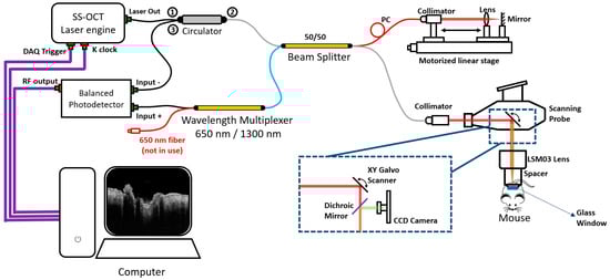
Figure 1.
The diagram of the hand-held Swept Source OCT system used for pre-acquired datasets. “①”, “②”, and “③” close to “Circulator” are the Port 1, 2, and 3 of the circulator; CCD: charge-coupled device; PC: polarization controller.
Each pre-acquired dataset contains 340 × 600 × 600 × 4 voxels (z–x–y–N, where z is the axial axis, x and y are the transverse axis, and N is the repeated times). The software operation of this system was performed through a LabVIEW program, while the post-processing was performed on MATLAB, which was implemented on a Windows 10 computer using an i9-10980XE (3.00 GHz) processor with random access memory (RAM) of 128 GB.
2.3. Mathematics for wED
As wED is a new approach to the ED reconstruction process, the OCTA scanning protocol for wED is the same as the aED [11,12]. The B scans were applied at the same locations a number of times. Therefore, each A-scan signal, , would contain both the depth and temporal information, which can be presented by:
where is the total depth of each A-scan, is the number of acquisitions at the same scanning location, and and are both integers. After applying a window, the windowed signal can be represented by:
where is the window’s position, and is the window size. The applied window would move from the first pixel towards the th pixel. Since the temporal information is contained in W, the windowed signal can also be presented as:
where is the structure component, is the flow component, and is the noise component, e.g., white noise. The aim of ED analysis is to extract . When is assumed to be Gaussian, the raw signals can be completely characterized by its correlation matrix, , given by:
where is the structure correlation matrix, is the flow correlation matrix, is the noise variance, and is the identity matrix [11,36,41]. The correlation matrix of the raw data can be estimated by:
where is the Hermitian transpose operation [11,12]. In this study, the structure component was assumed to be the dominant component within the input data . The dominant component can be separated by ED with the estimated raw data correlation matrix, which can be estimated by:
where is the unitary matrix of eigenvectors, and is the diagonal matrix of eigenvalues. The eigenvalues were sorted in descending order as the output of eigen-decomposition, pairing with the eigenvectors. More dominant components contribute to larger eigenvalues. Hence, the structure component was corresponding to the first th eigenvectors. Then, the flow component was extracted by:
where is an integer between 1 and [11,12]. The value of can be manually set to a fixed value or automatically set based on the eigenvalues. In this study, the total number of acquisitions at the same location, , was 4, while was set to be a fixed value, 2. Lastly, the windowed flow signals were combined into one A-scan flow signal, which was calculated by:
By averaging the results from all windows, the final flow component was the wED OCTA result for each A-scan.
To summarise, wED applies a moving window to the OCTA data then the ED analysis to extract blood flow signals from static tissue signals. In order to utilize the best window size during the processing, an optimization process was applied in this study. In total, 20 datasets were selected, spanning all stages of wound healing. The method for evaluating the window sizes was to calculate the correlation coefficients between the windowed input data distribution and the fitted normal distribution. After applying 35 various window sizes from 5 to 175 pixels, the window size generating the best average correlation coefficient was selected to be used in the wED algorithm, which will be demonstrated in the Results section.
2.4. Evaluation Method
In this study, Peak Signal-to-Noise Ratio (PSNR) was used to evaluate the performance of the wED algorithm. Within the calculation of PSNR, the input image is the image with noise, while the reference image is considered to be the desired signals only. The output, PSNR values were calculated as:
where is the maximum value of the input image data, and is the mean square error (MSE) between the input image and the reference image [42,43]. The MSE is calculated as:
where is the input data, is the reference data, and is the total number of data points [44]. The PSNR values would be related to how close the input image is to the signal-only reference image. The PSNR values were used to evaluate the performance of algorithms.
In in vivo studies, ground truth data are often unavailable. Therefore, in this study, the automatic registration [35] process from four successive acquisitions was applied to generate the reference data for quantitative evaluation. The four-time registration result would contain low noise and low motion artifacts, even though it had taken a long acquisition time. The automatic registration process utilized both rigid affine registration and nonrigid B-spline registration, using an open-source program, Elastix [45,46]. The simplified registration model [35] is explained as follows. When registration is applied to the input image, , and the reference image, , the transformation matrix, , can be defined as:
where is the special location of any pixel, and is the displacement caused by motion effects. Note that we only use one dimension, , for simplicity, while should be used in three-dimensional applications. In addition, the optimized transformation matrix, , under a cost function, , is:
where is the parameters vector, which contains parameters for both affine and B-spline transformation. After finding the best parameters vector with an adaptive stochastic gradient descent (ASGD) method, the registration process can be applied with weighting and averaging [35]. The registration process in this study was applied on MATLAB, whose results were used as the reference image when calculating PSNR.
3. Results
Pre-acquired SSOCT datasets from wound healing monitoring were used to evaluate wED and to compare wED with other OCTA reconstruction algorithms (SV, aED, bED) quantitatively and qualitatively.
3.1. Data Distribution Analysis
We discovered that the repeated acquired data in one B-frame were not normally distributed, as required by the ED analysis. One B-frame with four repeated scans was randomly chosen to apply the data distribution analysis to, with different selections of depth ranges after being flattened. This is shown in Figure 2. Here, we processed the distributions of the windowed B-scan frame, not A-lines, because there would be too few data points on each A-line to generate the distributions after applying the windows. The distributions of the selected data were plotted on the right, which were used to generate a fitted Gaussian. Lastly, for each window, the correlation coefficients between the distribution and the fitted Gaussian were calculated. In Figure 2, region of interest (ROI) (A), (B), (C), and (D) were the windows applied to the same B-scan frame. The axial windows’ sizes were 340, 170, 40, and 5 pixels in depth, respectively, which generated corresponding correlation coefficients of 0.67, 0.86, 0.99, and 0.72. Therefore, applying a window to the input data can improve the performance of ED statistical analysis, though the smallest window did not necessarily produce the best results.
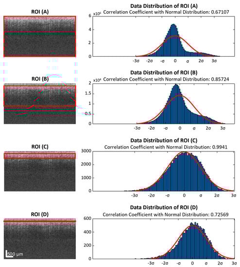
Figure 2.
ROIs (red rectangles) with different depth ranges were applied to the same flattened raw data. The selected data were plotted in histograms, which were compared with fitted normal distributions. (A) All data from the slice, which were 4 repeated B-scans contributing a 340 × 600 × 4 matrix. (B) A large ROI with half of the depth range, 170 pixels, was selected. (C) A small ROI with a depth range of 40 pixels. (D) An extremely small depth range of 5 pixels. ROI: region of interest.
3.2. Window Size Optimization
Before applying wED, an optimization process for window size was applied to all stages of wound healing. The result is shown in Figure 3. In Figure 3, the y-axis is for the normal-distribution correlation coefficients, while the x-axis is for the axial window sizes in pixels. The standard errors for all window sizes were displayed as the error bars in Figure 3. The optimized window size was utilized in wED.
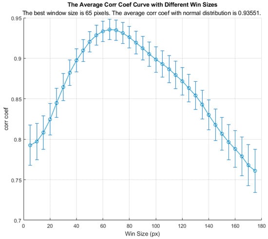
Figure 3.
The average normal-distribution correlation coefficients with different window sizes.
3.3. In Vivo Results Comparisons
After setting the optimized window size for the wED algorithm, several other algorithms, aED [11,12], bED [12], and SV [7] were used to evaluate the performance of wED. In Figure 4, the same B-frame was processed with SV, aED, bED, and wED, which were shown in (A), (B), (C), and (D), respectively. Since only aED and wED could resolve blood flow signals, the background noise intensities of aED and wED results in Figure 4 were calculated by averaging the intensity within the regions that contained no OCTA signals (deep regions). The wED result had a noise intensity of 0.259, while the aED contributed to a noise intensity of 0.316.
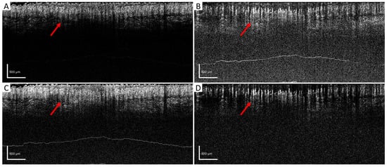
Figure 4.
B-scan comparison. The same B-scan frame with 4 repeating times was processed by (A) SV, (B) aED, (C) bED, and (D) wED, respectively. Regions that have differences in OCTA reconstruction were pointed out with red arrows. SV: Speckle Variance; aED: A-scan eigen-decomposition; bED: B-scan eigen-decomposition; wED: windowed eigen-decomposition.
For further evaluation, en face results were generated by using maximum intensity projection (MIP) within the papillary dermis layers, which contained dense and small blood vessels when observing the pre-acquired data. In order to compare the algorithms quantitatively, a ground truth is desired. However, one is not available for in vivo studies. Therefore, we utilized a four-time registration result as the alternative ground truth. Four successive acquisitions at the same scanning location were processed by aED, then registered into one 3D dataset using the Elastix registration toolbox [45,46]. The four-time registration result would contain low noise and low motion artifacts, even though it had taken a long acquisition time. Hence, the four-time registration result was used as the reference image when calculating the PSNR values. In Figure 5, the same MIP processing was applied to all processed blood-flow datasets from (A) four-time registration, (B) SV, (C) aED, (D) bED, and (E) wED. For each processing method, three regions were enlarged to observe the algorithms’ performance more clearly. Additionally, to present wED’s consistent performance, two alternative datasets from different stages of wound healing were processed to generate the same comparisons with that in Figure 5, which are presented in Appendix A Figure A1 and Figure A2.
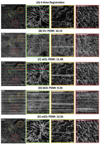
Figure 5.
The comparisons of en face results from maximum intensity projection using different algorithms. (A) Registration from 4-time acquisitions; (B) SV; (C) aED; (D) bED; (E) wED. (All scale bars represent 500 μm); SV: Speckle Variance; aED: A-scan eigen-decomposition; bED: B-scan eigen-decomposition; wED: windowed eigen-decomposition.
4. Discussion
We proposed a novel and easy-to-deploy wED that applies a moving window to the repeated scanned data. Compared to other popular OCTA reconstruction algorithms (SV, aED, bED), wED was less sensitive to motion artifacts and could better reduce background noise intensity.
To have wED at its best performance, the optimization of the moving window size played a vital role. The optimization result in Figure 3 indicates that the correlation coefficient between the raw data and the fitted normal distribution decreased as the axial window size increased over 65 pixels, though it also declined when the window size was smaller than 65 pixels. Therefore, a large depth range can affect the data distribution. However, the wED still requires static signals to be the dominant component. As a result, an extremely small window size would not be suitable either. Hence, the optimized window size was 65 pixels indicated in Figure 3, where the average normal-distribution correlation coefficient was 0.94.
Figure 4 shows the direct comparison of the cross-sectional B-frame. The arrows show how high-density blood vessels were resolved by different algorithms. Due to the high motion effects within the raw data, SV and bED could barely resolve any blood-flow information. Although both aED and wED could resolve the blood vessels, wED contains 18% less background noise according to the background noise intensity calculations.
In Figure 5, the en face and quantitative comparisons among four-time registration, SV, aED, bED, and wED are shown. With the four-time registration result as the ground truth, the PSNR was calculated for each algorithm to be evaluated (shown in Figure 5). The proposed wED had the highest PSNR value, 12.01, while the second highest is from aED, 11.48, which indicates the proposed approach wED has improved the reconstruction performance by 4.6%. Note that sometimes the aED results could have a higher PSNR when wED results were visually better, because the four-time registration result was not a perfect ground truth. Due to its long acquisition time (four times of a normal OCTA scan), the four-time registration result could have transformations (moving, translation, rigid, affine, and B-spline) of the vessel structure. As a result, the aED with higher background intensity could have a higher PSNR value instead. Visual judgment in Figure 5 could also match the quantitative results. To demonstrate the detailed visual difference among these algorithms, three areas in all en face results were enlarged as green, yellow, and red regions. SV could hardly resolve any blood-flow signals due to high motion effects. Although bED had some blood signals underneath the horizontal motion artifacts, these artifacts were too many to present any vessel networks. Matching with the B-scan comparison, only aED and wED were able to resolve most of the blood-flow signals. For the green region, wED could still generate less background noise, which provided better contrast of the blood vessels. Within the yellow region, a breathing motion artifact occurred. The bright horizontal lines could be observed in the aED result. In the wED result, while the breathing artifact did not disappear, it was reduced compared to the aED. In the red region, wED had better contrast of small vessels compared to aED. In addition, some motion artifacts still existed in the aED result, while they could hardly be seen from wED.
Although our approach of wED can outperform other algorithms, the tradeoff is the computation cost, which was measured as the processing time. To measure the processing time, the aED and wED algorithms were run in MATLAB on a Windows 10 computer using an i9-10980XE (3.00 GHz) processor with RAM of 128 GB. In total, 20 datasets of 340 × 600 × 600 × 4 (z-x-y-N) were processed, whose processing time was averaged. For each dataset, the wED algorithm would take 279.3 s on average, while aED only needed 98.6 s. However, as a post-processing algorithm, the computation cost can be sacrificed for better performance on OCTA.
Our proposed approach for OCTA reconstruction offers a reliable and convenient solution despite its computational cost limitations. Our method demonstrated superior performance compared to other reconstruction algorithms in both cross-sectional and en-face results. Additionally, the wED algorithm is able to effectively reduce motion artifacts and background noise. This study also serves as a guide for optimizing the wED algorithm when implementing it in practice.
5. Conclusions
We have proposed a new approach to eigen-decomposition as an essential reconstruction method for OCTA, which is windowed-ED (wED). The wED algorithm can be used to extract blood-flow signals from repeated scanning at the same position. This algorithm can reduce motion artifacts and improve PSNR performance compared to other algorithms for OCTA. Therefore, wED can be used for both animal models and human participants, especially when motion effects occur. This study can also be served as a guide for others to utilize our new, optimized, and easy-to-deploy wED algorithm.
Author Contributions
Conceptualization, T.Z. and K.Z.; methodology, T.Z.; software, T.Z.; validation, T.Z., K.Z., C.L. and Z.H.; formal analysis, T.Z.; investigation, T.Z., K.Z., H.R.R. and A.P.; resources, H.R.R. and A.P.; data curation, T.Z.; writing—original draft preparation, T.Z.; writing—review and editing, W.W., Z.W., C.L. and Z.H.; visualization, T.Z.; supervision, C.L. and Z.H.; project administration, K.Z., J.L.C., C.L. and Z.H.; funding acquisition, J.L.C. and Z.H. All authors have read and agreed to the published version of the manuscript.
Funding
The establishment of the mouse model was funded by a Wellcome Trust and Royal Society Sir Henry Dale Fellowship to Dr. Cash (202581/Z/16/Z), and a Chancellors Fellowship PhD studentship, which was funded through Dr. Cash’s fellowship, to Dr. Holly Rocliffe.
Institutional Review Board Statement
All animal procedures were performed under PIL I61689163 and PPL PD3147DAB (January 2018–January 2021) and conducted with approval from the local ethical review committee at the University of Edinburgh and under UK Home Office regulations (Guidance on the Operation of Animals, Scientific Procedures Act, 1986).
Informed Consent Statement
Not applicable.
Data Availability Statement
The data presented in this study are available on request from the corresponding author. The data are not publicly available due to ethical restrictions.
Acknowledgments
We would like to express our gratitude to Yilong Zhang, Yubo Ji, and Jinpeng Liao for their supports.
Conflicts of Interest
The authors declare no conflict of interest.
Appendix A

Figure A1.
The comparisons of en face results from maximum intensity projection. (A) Registration from 4-time acquisitions; (B) SV; (C) aED; (D) bED; (E) wED. (All scale bars represent 500 μm); SV: Speckle Variance; aED: A-scan eigen-decomposition; bED: B-scan eigen-decomposition; wED: windowed eigen-decomposition.

Figure A2.
The comparisons of en face results from maximum intensity projection using different algorithms. (A) Registration from 4-time acquisitions; (B) SV; (C) aED; (D) bED; (E) wED. (All scale bars represent 500 μm); SV: Speckle Variance; aED: A-scan eigen-decomposition; bED: B-scan eigen-decomposition; wED: windowed eigen-decomposition.
References
- Aumann, S.; Donner, S.; Fischer, J.; Müller, F. Optical Coherence Tomography (OCT): Principle and Technical Realization. In High Resolution Imaging in Microscopy and Ophthalmology; Springer: Cham, Switzerland, 2019; pp. 59–85. [Google Scholar] [CrossRef]
- Tomlins, P.H.; Wang, R.K. Theory, Developments and Applications of Optical Coherence Tomography. J. Phys. D Appl. Phys. 2005, 38, 2519. [Google Scholar] [CrossRef]
- Fercher, A.F.; Drexler, W.; Hitzenberger, C.K.; Lasser, T. Optical Coherence Tomography—Principles and Applications. Rep. Prog. Phys. 2003, 66, 239. [Google Scholar] [CrossRef]
- Chen, C.-L.; Wang, R.K. Optical Coherence Tomography Based Angiography [Invited]. Biomed. Opt. Express 2017, 8, 1056–10828. [Google Scholar] [CrossRef] [PubMed]
- Schwartz, D.M.; Fingler, J.; Kim, D.Y.; Zawadzki, R.J.; Morse, L.S.; Park, S.S.; Fraser, S.E.; Werner, J.S. Phase-Variance Optical Coherence Tomography: A Technique for Noninvasive Angiography. Ophthalmology 2014, 121, 180–187. [Google Scholar] [CrossRef]
- Leitgeb, R.A.; Werkmeister, R.M.; Blatter, C.; Schmetterer, L. Doppler Optical Coherence Tomography. Prog. Retin. Eye Res. 2014, 41, 26. [Google Scholar] [CrossRef]
- Mariampillai, A.; Standish, B.A.; Moriyama, E.H.; Khurana, M.; Munce, N.R.; Leung, M.K.K.; Jiang, J.; Cable, A.; Wilson, B.C.; Vitkin, I.A.; et al. Speckle Variance Detection of Microvasculature Using Swept-Source Optical Coherence Tomography. Opt. Lett. 2008, 33, 1530. [Google Scholar] [CrossRef]
- Jia, Y.; Tan, O.; Tokayer, J.; Potsaid, B.; Wang, Y.; Liu, J.J.; Kraus, M.F.; Subhash, H.; Fujimoto, J.G.; Hornegger, J.; et al. Split-Spectrum Amplitude-Decorrelation Angiography with Optical Coherence Tomography. Opt. Express 2012, 20, 4710. [Google Scholar] [CrossRef]
- Enfield, J.; Jonathan, E.; Leahy, M. In Vivo Imaging of the Microcirculation of the Volar Forearm Using Correlation Mapping Optical Coherence Tomography (CmOCT). Biomed. Opt. Express 2011, 2, 1184. [Google Scholar] [CrossRef]
- Braaf, B.; Donner, S.; Nam, A.S.; Bouma, B.E.; Vakoc, B.J. Complex Differential Variance Angiography with Noise-Bias Correction for Optical Coherence Tomography of the Retina. Biomed. Opt. Express 2018, 9, 486. [Google Scholar] [CrossRef]
- Yousefi, S.; Zhi, Z.; Wang, R.K. Eigendecomposition-Based Clutter Filtering Technique for Optical Microangiography. IEEE Trans. Biomed. Eng. 2011, 58, 2316–2323. [Google Scholar] [CrossRef]
- Zhang, Q.; Wang, J.; Wang, R.K. Highly Efficient Eigen Decomposition Based Statistical Optical Microangiography. Quant. Imaging Med. Surg. 2016, 6, 557–563. [Google Scholar] [CrossRef] [PubMed]
- Abu-Yaghi, N.E.; Obiedat, A.F.; Alnawaiseh, T.I.; Hamad, A.M.; Bani Ata, B.A.; Quzli, A.A.; Alryalat, S.A. Optical Coherence Tomography Angiography in Healthy Adult Subjects: Normative Values, Frequency, and Impact of Artifacts. Biomed. Res. Int. 2022, 2022, 7286252. [Google Scholar] [CrossRef] [PubMed]
- Liba, O.; Lew, M.D.; Sorelle, E.D.; Dutta, R.; Sen, D.; Moshfeghi, D.M.; Chu, S.; de La Zerda, A. Speckle-Modulating Optical Coherence Tomography in Living Mice and Humans. Nat. Commun. 2017, 8, 15845. [Google Scholar] [CrossRef] [PubMed]
- Jian, Y.; Zawadzki, R.J.; Sarunic, M.V. Adaptive Optics Optical Coherence Tomography for in Vivo Mouse Retinal Imaging. J. Biomed. Opt. 2013, 18, 056007. [Google Scholar] [CrossRef] [PubMed]
- Merkle, C.W.; Cooke, D.F.; Radhakrishnan, H.; Krubitzer, L.; Chong, S.P.; Zhang, T.; Srinivasan, V.J. Noninvasive, in Vivo Imaging of Subcortical Mouse Brain Regions with 1.7 μm Optical Coherence Tomography. Optics. Lett. 2015, 40, 4911–4914. [Google Scholar] [CrossRef]
- Kim, T.H.; Son, T.; Lu, Y.; Alam, M.; Yao, X. Comparative Optical Coherence Tomography Angiography of Wild-Type and Rd10 Mouse Retinas. Transl. Vis. Sci. Technol. 2018, 7, 42. [Google Scholar] [CrossRef]
- Zhi, Z.; Chao, J.R.; Wietecha, T.; Hudkins, K.L.; Alpers, C.E.; Wang, R.K. Noninvasive Imaging of Retinal Morphology and Microvasculature in Obese Mice Using Optical Coherence Tomography and Optical Microangiography. Invest. Ophthalmol. Vis. Sci. 2014, 55, 1024–1030. [Google Scholar] [CrossRef]
- de Carlo, T.E.; Romano, A.; Waheed, N.K.; Duker, J.S. A Review of Optical Coherence Tomography Angiography (OCTA). Int. J. Retin. Vitr. 2015, 1, 1–15. [Google Scholar] [CrossRef]
- Ghasemi Falavarjani, K.; Al-Sheikh, M.; Akil, H.; Sadda, S.R. Image Artefacts in Swept-Source Optical Coherence Tomography Angiography. Br. J. Ophthalmol. 2017, 101, 564–568. [Google Scholar] [CrossRef]
- Govindaswamy, N.; Gadde, S.G.; Chidambara, L.; Bhanushali, D.; Anegondi, N.; Sinha Roy, A. Quantitative Evaluation of Optical Coherence Tomography Angiography Images of Diabetic Retinopathy Eyes before and after Removal of Projection Artifacts. J. Biophotonics 2018, 11, e201800003. [Google Scholar] [CrossRef]
- Tomlinson, A.; Hasan, B.; Lujan, B.J. Importance of Focus in OCT Angiography. Ophthalmol. Retin. 2018, 2, 748–749. [Google Scholar] [CrossRef] [PubMed]
- Spaide, R.F.; Fujimoto, J.G.; Waheed, N.K. Image Artifacts in Optical Coherence Angiography. Retina 2015, 35, 2163. [Google Scholar] [CrossRef] [PubMed]
- Stepien, K.E.; Konda, S.M.; Etheridge, T.; Holmen, I.; Kopplin, L.; Pak, J.W.; Domalpally, A. Impact of Artifacts in Optical Coherence Tomography Angiography Image Analysis. Invest. Ophthalmol. Vis. Sci. 2020, 61, 4818. [Google Scholar]
- Lavinsky, F.; Lavinsky, D. Novel Perspectives on Swept-Source Optical Coherence Tomography. Int. J. Retin. Vitr. 2016, 2, 1–11. [Google Scholar] [CrossRef]
- Yasin Alibhai, A.; Or, C.; Witkin, A.J. Swept Source Optical Coherence Tomography: A Review. Curr. Ophthalmol. Rep. 2018, 6, 7–16. [Google Scholar] [CrossRef]
- Ren, J.; Park, K.; Pan, Y.; Ling, H. Self-Supervised Bulk Motion Artifact Removal in Optical Coherence Tomography Angiography. In Proceedings of the IEEE/CVF Conference on Computer Vision and Pattern Recognition, New Orleans, LA, USA, 19–24 June 2022; pp. 20617–20625. [Google Scholar]
- Xie, C.; Gao, W.; Zhang, Y. Fourier Spatial Transform-Based Method of Suppressing Motion Noises in OCTA. Optics. Lett. 2022, 47, 4544–4547. [Google Scholar] [CrossRef]
- Camino, A.; Jia, Y.; Liu, G.; Wang, J.; Huang, D. Regression-Based Algorithm for Bulk Motion Subtraction in Optical Coherence Tomography Angiography. Biomed. Opt. Express 2017, 8, 3053–3066. [Google Scholar] [CrossRef]
- Torti, E.; Toma, C.; Vujosevic, S.; Nucci, P.; de Cillà, S.; Leporati, F. Cyst Detection and Motion Artifact Elimination in Enface Optical Coherence Tomography Angiograms. Appl. Sci. 2020, 10, 3994. [Google Scholar] [CrossRef]
- Li, P.; Huang, Z.; Yang, S.; Ren, Q.; Li, P.; Liu, X. Adaptive Classifier Allows Enhanced Flow Contrast in OCT Angiography Using a Histogram-Based Motion Threshold and 3D Hessian Analysis-Based Shape Filtering. Opt. Lett. 2017, 42, 4816–4819. [Google Scholar] [CrossRef]
- Li, A.; Zeng, G.; Du, C.; Zhang, H.; Pan, Y. Automated Motion-Artifact Correction in an OCTA Image Using Tensor Voting Approach. Appl. Phys. Lett. 2018, 113, 101102. [Google Scholar] [CrossRef]
- Wei, D.W.; Deegan, A.J.; Wang, R.K. Automatic Motion Correction for In Vivo Human Skin Optical Coherence Tomography Angiography through Combined Rigid and Nonrigid Registration. J. Biomed. Opt. 2017, 22, 066013. [Google Scholar] [CrossRef] [PubMed]
- Camino, A.; Zhang, M.; Dongye, C.; Pechauer, A.D.; Hwang, T.S.; Bailey, S.T.; Lujan, B.; Wilson, D.J.; Huang, D.; Jia, Y. Automated Registration and Enhanced Processing of Clinical Optical Coherence Tomography Angiography. Quant. Imaging Med. Surg. 2016, 6, 391. [Google Scholar] [CrossRef] [PubMed]
- Cheng, Y.; Chu, Z.; Wang, R.K. Robust Three-Dimensional Registration on Optical Coherence Tomography Angiography for Speckle Reduction and Visualization. Quant. Imaging Med. Surg. 2021, 11, 879. [Google Scholar] [CrossRef] [PubMed]
- Yu, A.C.H.; Lovstakken, L. Eigen-Based Clutter Filter Design for Ultrasound Color Flow Imaging: A Review. IEEE Trans. Ultrason. Ferroelectr. Freq. Control 2010, 57, 1096–1111. [Google Scholar] [CrossRef] [PubMed]
- Mogensen, M.; Morsy, H.A.; Thrane, L.; Jemec, G.B.E. Morphology and Epidermal Thickness of Normal Skin Imaged by Optical Coherence Tomography. Dermatology 2008, 217, 14–20. [Google Scholar] [CrossRef]
- Welzel, J. Optical Coherence Tomography in Dermatology: A Review. Ski. Res. Technol. 2001, 7, 1–9. [Google Scholar] [CrossRef] [PubMed]
- Zhou, K.; Feng, K.; Li, C.; Huang, Z. A Weighted Average Phase Velocity Inversion Model for Depth-Resolved Elasticity Evaluation in Human Skin In-Vivo. IEEE Trans. Biomed. Eng. 2021, 68, 1969–1977. [Google Scholar] [CrossRef] [PubMed]
- Ji, Y.; Yang, S.; Zhou, K.; Rocliffe, H.R.; Pellicoro, A.; Cash, J.L.; Wang, R.; Li, C.; Huang, Z. Deep-Learning Approach for Automated Thickness Measurement of Epithelial Tissue and Scab Using Optical Coherence Tomography. J. Biomed. Opt. 2022, 27, 015002. [Google Scholar] [CrossRef]
- Kruse, D.E.; Ferrara, K.W. A New High Resolution Color Flow System Using an Eigendecomposition-Based Adaptive Filter for Clutter Rejection. IEEE Trans Ultrason. Ferroelectr. Freq. Control 2002, 49, 1384–1399. [Google Scholar] [CrossRef]
- Kendall, M.G. The Advanced Theory of Statistics; Charles Griffin and Co., Ltd.: London, UK, 1946. [Google Scholar]
- Fisher, R.A. Statistical Methods for Research Workers. In Breakthroughs in Statistics; Springer: New York, NY, USA, 1992; pp. 66–70. [Google Scholar] [CrossRef]
- Fürnkranz, J.; Chan, P.K.; Craw, S.; Sammut, C.; Uther, W.; Ratnaparkhi, A.; Jin, X.; Han, J.; Yang, Y.; Morik, K.; et al. Mean Squared Error. In Encyclopedia of Machine Learning; Springer: Boston, MA, USA, 2011; p. 653. [Google Scholar] [CrossRef]
- Marstal, K.; Berendsen, F.; Staring, M.; Klein, S. SimpleElastix: A User-Friendly, Multi-Lingual Library for Medical Image Registration. In Proceedings of the IEEE Computer Society Conference on Computer Vision and Pattern Recognition Workshops, Las Vegas, NV, USA, 26 June–1 July 2016; pp. 574–582. [Google Scholar] [CrossRef]
- Shamonin, D.P.; Bron, E.E.; Lelieveldt, B.P.F.; Smits, M.; Klein, S.; Staring, M. Fast Parallel Image Registration on CPU and GPU for Diagnostic Classification of Alzheimer’s Disease. Front. Neuroinform. 2014, 7, 50. [Google Scholar] [CrossRef]
Disclaimer/Publisher’s Note: The statements, opinions and data contained in all publications are solely those of the individual author(s) and contributor(s) and not of MDPI and/or the editor(s). MDPI and/or the editor(s) disclaim responsibility for any injury to people or property resulting from any ideas, methods, instructions or products referred to in the content. |
© 2022 by the authors. Licensee MDPI, Basel, Switzerland. This article is an open access article distributed under the terms and conditions of the Creative Commons Attribution (CC BY) license (https://creativecommons.org/licenses/by/4.0/).