Abstract
Accurate global horizontal irradiance (GHI) forecasting promotes power grid stability. Most of the research on solar irradiance forecasting has been based on a single-site analysis. It is crucial to explore multisite modeling to capture variations in weather conditions between various sites, thereby producing a more robust model. In this research, we propose the use of spatial regression coupled with Gaussian Process Regression (GP Spatial) and the GP Autoregressive Spatial model (GP-AR Spatial) for the prediction of GHI using data from seven radiometric stations from South Africa and one from Namibia. The results of the proposed methods were compared with a benchmark model, the Linear Spatial Temporal Regression (LSTR) model. Five validation sets each comprised of three stations were chosen. For each validation set, the remaining five stations were used for training. Based on root mean square error, the GP model gave the most accurate forecasts across the validation sets. These results were confirmed by the statistical significance tests using the Giacommini–White test. In terms of coverage probability, there was a 100% coverage on three validation sets and the other two had 97% and 99%. The GP model dominated the other two models. One of the study’s contributions is using standardized forecasts and including a nonlinear trend covariate, which improved the accuracy of the forecasts. The forecasts were combined using a monotone composite quantile regression neural network and a quantile generalized additive model. This modeling framework could be useful to power utility companies in making informed decisions when planning power grid management, including large-scale solar power integration onto the power grid.
1. Introduction
1.1. Overview
The use of energy sources that are clean and renewable has been on the rise, hence the need to efficiently manage the power grid. This increase has led to the need to come up with predictions of the available energy sources to ease the management of the power grid. Power grid planning is a challenging process, as it requires efficient and accurate power predictions inputs. In this research, we focused on probabilistic, short-term forecasting to efficiently model GHI. Probability forecasting is an emerging research area that handles the uncertainty of weather variables, which produces more comprehensive results [1]. This probability approach was combined with spatial analysis to assess the relatedness of meteorological stations. Spatial analysis is a very important aspect in regression, and in this study it was used to explore spatial dependence between various meteorological stations.
1.2. Survey of Related Literature
Some authors have applied various methods incorporating spatial analysis. Andre et al. [2] used a spatial–temporal model for short-term solar irradiation forecasting. They used a spatial–temporal vector autoregressive model, which was designed in such a way that it could handle sparse spatial–temporal data. An iterative strategy in the model process selected related stations and eliminated insignificant predictor variables.
In a study by Liu et al. [3], an ensemble-temporal deep learning approach incorporating multi-sites in a spatial power grid was used to predict solar power. Variational modeling was used to predict uncertainty, and the proposed methods estimated uncertainty very well. Yang [4] used the ultra-fast pre-selection method to solve the lasso problem, that of having an insufficient degree of freedom and curse of dimensionality. The variables selected via ultra-fast were then used to develop a lasso-temporal model. Their results showed that their proposed algorithm did not need meteorological priors and provided the best forecasts.
Another study by Eschenbach et al. [5] was based on forecasting solar irradiation based on various machine-learning methods. The methods used were ARX (autoregressive with exogenous inputs), NN (Neural Network), RRF (random regression forest), and RT (regression trees). Their results showed that for a short lead time, NN produced more accurate results as well as for dense-temporal input data.
Kim et al. [6] applied a temporal method that combined public and satellite data. Based on a satellite from South Korea, SVR (Support Vector Regression), ANN (Artificial Neural Network), ARIMAX (Autoregressive Moving Average), and DNN (Deep Neural Network) were used based on short interval forecasts of GHI data. Their results showed that the models based on temporal and spatial characteristics gave better forecasts than the other models that were based on numerical data using weather variables.
Zhang et al. [7] applied a Spatial–Temporal Gaussian process state space model with the Kronecker structure on weather data from Colorado and Global Historical Climatology Network. The other objective was to come up with a kernel that will be used for the Colorado and GHCN (Global Historical Climatology Network) data. To estimate the hyper parameters of the Spatial–Temporal Gaussian model, the Kalman Filter and smoother was used. The results showed that the forecasting performance improved from the results by [8] based on the desirable properties of the Matern kernel used for both datasets.
Hamelinjck et al. [9] applied variational spatio-temporal regression coupled with Gaussian processes. A non-conjugate GP technique produced a sparse state model using separable Markov kernels. The results of the proposed methodology proved to be more accurate and efficient due to filtering parallelization of spatial locations, sparsity, and application of variational Gaussian process analysis. The proposed method outperformed the baseline methods.
Agoua et al. [10] forecasted photovoltaics using a probabilistic spatial–temporal model approach that used datasets from plants that were close to each other. This technique incorporates short dry forecasting of periods of 0–6 h. Quantile regression was combined with Lasso, which was used for variable selection. The proposed methodology showed superior performance in comparison to KDE (Kernel Density Estimation), which was used as the benchmark model.
Banerjee et al. [11] developed a temporal–spatial model using predictive process modeling. The method reduced computational burden by reducing the modeling space to a lower dimensional subspace. The results of the proposed methodology addressed the problem of misspecification of the model using a larger dataset, which was achieved by applying the induced specification predictive process.
Luttinen et al. [12] did a Bayesian analysis using sea surface temperature data. They used a probabilistic factor analysis using spatiotemporal data. Gaussian process priors were used for the factors and loading matrix. According to their results, the Gaussian Process Factor Analysis outperformed the Bayesian Principal Component analysis.
Tomizawa and Yoshida [13] applied Gaussian Process regression with various Gaussian random fields to data with problems of spatial variability. The maximum likelihood method was used to estimate the random and fluctuating fields’ scale. Their results showed that the model with the Whittle Matern kernel was the best for the random component.
Comber et al. [14] used Gaussian Process splines regression taking into account the variational of geographical areas. The technique is a smoothing parameter used in splines regression combined with Gaussian Processes, optimizing the GP splines regression. The model showed predictions that were more accurate because of accommodating heterogeneity.
Another research was done by Najimbi et al. [15], they used probabilistic GPR to forecast solar power using meteorological data. Short-term forecasting was used based on k-means clustering. A Matern covariance function was used. A 5-fold validity test set, holding out 30 random days, was used to validate the applied method. Root mean square error was reduced due to the application of the proposed methodology.
In another paper, Najimbi et al. [16] predicted solar power using weather variables. Eight different partitions were used to cluster the data using k-means clustering, and GPR was used based on the Matern covariance function. The Elbow and Gap techniques were used to develop optimal clusters, and the results showed that the forecasting error was reduced.
Paiva et al. [17] performed a comparative analysis on multilayer perceptron (MLP) artificial neural networks and multigene genetic programming (MGGP). The assessments indicated that MGGP gave more accurate and fast results in single predictions, and the ANN performed better for ensemble forecasts. Wang et al. [18] used a cluster-based analysis on ultra-short-term wind power using a hierarchical directed graph method and dynamic–temporal correlation. They first defined three nodes based on wind power, wind speed, and target nodes, and defined input sample and correlation matrices that are temporal-based to evaluate the correlation of neighboring wind farms. They also used directed edges to connect various nodes to obtain a hierarchical-based graph form, which was later applied to train the prediction model. The proposed model outperformed the other benchmark models used.
The world meteorological organization produced a guide highlighting the major sources of uncertainty in forecasted values related to the weather as the process of producing a forecast, its interpretation, and atmospheric unpredictability (Gill et al. [19]). Most of the studies reviewed in this research on forecasting global horizontal irradiance (GHI) using spatial regression considered only the spatial feature, leaving out weather variables and the variability in GHI. Additionally, most classical approaches for predicting GHI rely mainly on a single power plant. The current study focuses on a multi-site approach to modeling and forecasting GHI using Gaussian process models and including a nonlinear trend covariate. A summary of previous studies on modeling solar radiation based on spatial analysis is given in Table 1.
Table 1.
Summary of some previous studies on temporal dependence modeling of GHI.
1.3. Research Highlights and Contributions
The current study presents an in-depth analysis and spatial–temporal predictive modeling of GHI at radiometric stations in sparse geographical regions. To the best of our knowledge, this is the first study to be carried out using South African data. The study proposes the standardization of predictions, which improves forecast accuracy. Another highlight is in the selection of the validation sets. Eight radiometric stations were used in the study, with three locations in each validation set. This resulted in fifty six possible validation sets. From the randomly selected five sets, an in-depth analysis was carried out to investigate how the proposed models would perform, especially those stations that are far apart in Euclidean space.
Based on the literature review discussed in Section 1.2, the highlights and contributions made in this study are summarized as follows. The research focused on moving from a single site to a multi-site forecasting approach, that is, using geographically sparse data. Multi-site research is expected to give a diverse or large sample that is good enough to come up with significant associations between meteorological stations; hence, it enhances the statistical power of the model. Previously, solar forecasting has been based on single-site analysis. Exploring the temporal forecasting approach is expected to improve modeling accuracy.
We predicted solar irradiation using spatial regression coupled with Gaussian process modeling using Bayesian inference. GP regression has proved to be a very powerful tool for modeling the variability and uncertainty of solar irradiation [20], though it is very computationally expensive. The spatial analysis then improves the predictive accuracy since it reduces the computational burden in regression analysis. The combination of these two methods thus produces a hybrid model that produces favorable results.
A comparative analysis was done between the proposed models, GP Spatial and GP-AR Spatial, and the linear spatial model, which was used as a benchmark model. The evaluation metrics used to assess the accuracy of the models are MAE (Mean Absolute Error), RMSE (Root Mean Square Error), CP (Coverage Probability) and CRPS (Continuous Rank Probability Score).
Standardization of the forecasts made from the selected model was also done in this research. The standardized forecasts were then added to the original forecasts, improving the forecast accuracy. During forecasting, multicollinearity can be introduced if independent variables are correlated. This problem compromises the model’s statistical significance and produces imprecise coefficients. To overcome this problem, we used ElaticNet, one of the shrinkage methods used in variable selection. ElaticNet is a supervised algorithm that identifies the variables strongly associated with the response variable. The nonlinear rend variable is another important variable that resulted in a significant improvement in the forecast accuracy. Finally, we combined forecasts using QGAM (Quantile Generalized Additive Model) and MCQRNN (Monotone Composite Quantile Regression Neural Networks). Combining forecasts is a very effective tool for reducing errors.
The following sections are organized as follows. Section 2 briefly discusses the temporal GP and GP-temporal autoregressive models, including the benchmark model Linear-temporal Regression. The section also presents a discussion of Bayesian inference, which is used in the computation of the parameters. The results of the exploratory analysis of GHI proposed methods and the benchmark model are given in Section 3. The conclusion is given in Section 4.
2. Methodology
2.1. Flowchart
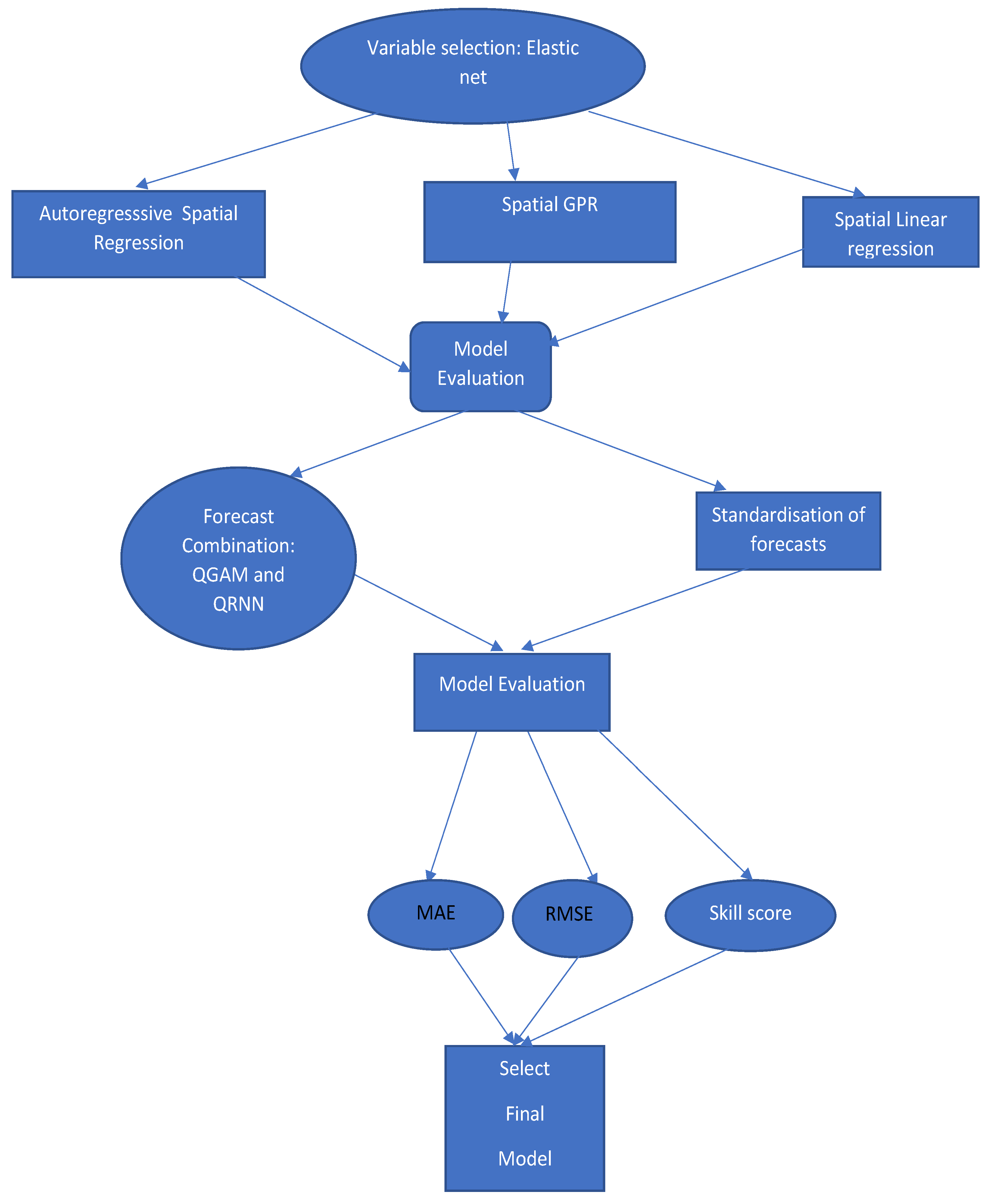
The flow chart of the structure of the paper outlining the proposed models and evaluation metrics is shown in Figure 1. Two proposed models, the spatial–temporal Gaussian (GP) regression model and GP coupled with autoregressive (GP-AR) error terms, are compared with a benchmark model, the spatial–temporal linear regression model. The performance of the models is evaluated using the root mean square error (RMSE), mean absolute error (MAE), and skill score (SS).
Figure 1.
Flow chart of the structure of the paper.
2.2. Variable Selection
In order to select significant variables for the analysis, ElasticNet, a regularization technique, was used [21]. ElasticNet is a shrinkage method that uses penalties from ridge regression () and Lasso regression () to reduce the number of variables in a regression model. It combines both ridge and Lasso methods to overcome their limitations. Elastic net minimizes the function in Equation (1).
where is the mixing parameter that is between lasso, and ridge, , is the regularization penalty parameter, is the response variable, and is a vector of parameters.
2.3. Spatio-Temporal Gaussian Process Regression Model
Gaussian processes were developed by Williams and Rasmussen [22]. Gaussian processes can be presumed as elements of spatial–temporal modeling because these stochastic processes are defined, in this case, over a given region where the stations have different locations. The spatial analysis aims to develop the best model to produce a set of outputs using inputs from various locations at different time frames. A temporal Gaussian process (GP) model is given in Equation (2).
where is the spatially-dependent error term (spatio-temporal process), represents the response variable (GHI) at station at time t, for ; with representing the covariates, is a vector of constants and is the pure random error term. Gaussian processes are characterized by the covariance (kernel) functions. Various kernel functions can be used, but the Matern and squared exponential are commonly used. In this study, the Matern covariance kernel was used because it gives a better balance between the roughness and smoothness of the developed model. The temporal process is assumed to be a GP with the Matern covariance function given in Equation (3)
where d represents the distance between two points, is the modified Bessel function of the second kind and and are parameters. That is
The GP model can be represented hierarchically as shown in Equation (5).
where assuming and with representing the sample covariance matrix.
The prior distribution assumes a normal distribution as shown in Equation (6).
The posterior distribution is given in Equation (7).
where is the 1-step ahead forecast and is an unobserved location at time . The hyperparameters are solved by maximizing the marginal likelihood function given in Equation (8).
where is the noise variance, represents the hyperparameters and is the covariance function. The posterior predictive distribution of given y is given in Equation (9).
where is the joint posterior distribution of and . This study uses the GP temporal approach to forecasting solar irradiance.
2.4. Gaussian Process Regression Based Autoregressive Model
Another approach to forecasting solar irradiance in this research is the autoregressive (AR) spatio-temporal model. The Gaussian process autoregressive model [23] is given hierarchically as shown in Equation (10).
where assuming and with representing the sample covariance matrix as given in Section 2.3.
Parameters of the spatio-temporal AR model are computed based on prior distributions. The data types are used to group the parameters: mean, variance and correlation. Parameters like and describing the mean are classified under independent normal prior distributions. The means are specified as () and their variances are (). The independent normal distribution is for each component of the n-dimensional vector of the autoregressive model.
The likelihood function is given in Equation (11).
where is the covariance vector and is the covariance matrix and are hyperparameters for mean and variance. The posterior distribution is given by (12).
where
The posterior predictive distribution is given in Equation (13).
where is a spatial process that captures spatial association, is an independent process and are the weather-related variables.
2.5. The Linear Spatial Model
The linear spatial model is given in Equation (14).
where is an error term with a zero-mean spatio-temporal Gaussian process with a covariance structure given in Equation (15).
where represents an isotropic correlation function [23].
A summary of the advantages and disadvantages of the proposed methods is given in Table 2.
Table 2.
Model comparisons of the proposed techniques.
2.6. Averaging Forecasts
It is well established in the literature that combining forecasts improves forecast accuracy. This study combines forecasts with two models, the monotone composite quantile regression neural network (MCQRNN) and the QGAM.
Given the forecasts , from models and the combined forecasts , MCQRNN seeks to minimize the loss function given in Equation (16).
where
is the conditional quantile of y at and is a vector of unknown parameters. For a detailed discussion of MCQRNN, see [24,25], among others.
QGAM is a hybrid model that is a combination of generalized additive (GAM) and quantile regression (QR) models. QGAMs were developed by Fasiolo et al. [26]. The QGAM model is given in Equation (17)
where is the pinball loss function.
2.7. Deterministic Evaluation Metrics
Four techniques were used to evaluate the models: two are deterministic, and two are probabilistic. RMSE (Root Mean Square Error) and MAE (Mean absolute error) were the error measures used. The two forecast evaluation metrics are given in Equations (18) and (19), respectively.
where m is the number of forecasts, is GHI and the predictions of GHI are denoted by . The RMSE given in Equation (18) is used in this study to determine the forecast skill (), which helps in benchmarking the forecast quality of the models to the naive model (the model based on unstandardized forecasts). The forecasting skill is given in Equation (20).
where is a measure of the superiority of the forecast of the developed model to the forecast of the naive (benchmark) model. The best model is one that gives the highest value of the positive percentage change.
2.8. Probabilistic Evaluation Metrics
Continuous ranked probability score (CPRS) and coverage probability (CP) are probabilistic evaluation metrics used to measure forecasts’ performance. They consider the distributions of the forecasted values as a whole.
where are the predictions, F is the cumulative distribution function (CDF) of Y, and are two independent copies of the linear variables, and are their respective values, that are distributed with respect to F. Now, with m validation observations, the score is calculated as
where
The CP probability is given Equation (23).
where denotes the predictive interval for the prediction and denotes the indicator function, which takes the value one when and zero otherwise. The four techniques were used to evaluate the GP, GP-AR, and linear spatio-temporal models.
2.9. Statistical Significance
To assess the significance of differences in forecast accuracy of a pair of two competing forecasts of models f and h, we use the Diebold Mariano (DM) and Giacomini White (GW) tests.
2.9.1. Diebold-Mariano Test
The Diebold and Mariano [27] test is used to test for the unconditional predictive ability of two competing forecasts from models A and B.
Let be GHI at site i, at time t and two forecasts . Assuming the errors from the forecasts are defined as . If is an error loss function, then a loss function which penalizes underprediction more heavily than overprediction as suggested by [28] is given as (24):
The loss differential is then calculated as [28]:
The null hypothesis states that the two sets of forecasts have the same accuracy and is given as , and the alternative is
2.9.2. Giacomini-White Test
The GW test generalizes the DM test [29]. The GW has the added advantage of accounting for uncertainty in estimating parameters. It tests the conditional predictive ability of a competing pair of forecasts. The test considers the regression given in Equation (26).
where has elements from the information set on day , with the pair of forecasts from models f and h. The differential series is the same as that of the Diebold Mariano test. The CPA test is then computed with the null hypothesis in the regression given in Equation (26).
2.10. Standardization of the Forecasts
Standardization of data scales forecasts to the same range of values to improve the predictions’ quality. This creates consistency in the dataset by avoiding wider ranges from the data. The forecasts are standardized using Equation (27).
where are the forecasts at each station i at time t, is the mean value of the forecasts and is the standard deviation of GHI forecasts. The new adjusted forecasts will therefore be given by
3. Empirical Results
3.1. Data Used in the Study
The dataset used in this study was collected from the SAURAN (Southern African Universities Radiometric Network) website https://sauran.ac.za/, accessed on 13 August 2022. Eight radiometric stations were selected for the study. These were the only radiometric stations from SAURAN that had clean data for the sampling period used. However, future research will include the use of satellite data and more stations, including the use of gridded data covering the whole country.
The stations are CSIR—CSIR Energy Centre (1), CUT-Central University of technology (2), UFH-University of Fort Hare (3), UNV-University of Venda (4), UNZ-University of Zululand (5), UPR-University of Pretoria (6), MIN-CRSES Mintek (7) and NUST-Namibian University of Science and Technology (8). The covariates used in the study are temperature, relative humidity, wind speed, wind direction, wind direction standard deviation, barometric pressure, month, day, noltrend (nonlinear trend variable), elevation, and the dependent variable GHI. R statistical software was used for all the analyses that were done in this study.
The modeling and analysis were done using a Dell laptop with the following specifications: 8GB RAM, processor Intel(R) Core(TM) i5-10210U CPU @ 1.60GHz 2.11 GHz, 64-bit operating system, x64-based processor.
3.2. Exploratory Data Analysis
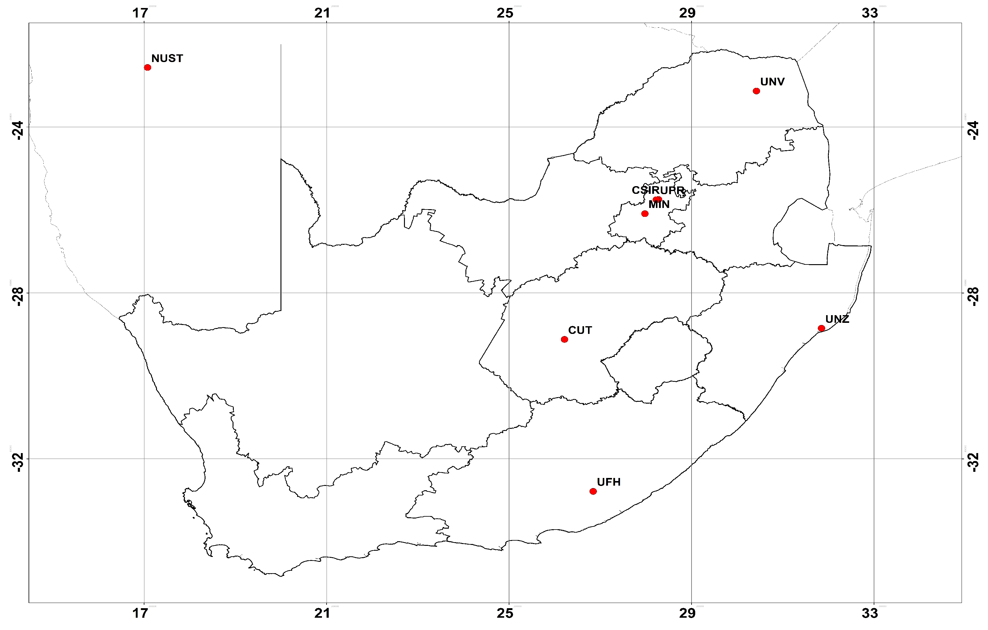
The locations of the eight radiometric stations used in this study are given in Figure 2.
Figure 2.
Map showing radiometric stations. Source: Author’s creation.
The longitudes, latitudes and elevations of the eight radiometric stations shown in Figure 2 are presented in Table 3a. Table 3b summarizes the distances between radiometric stations. The bottom left of the leading diagonal shows the distance between stations, while the top right shows the pairwise Kendall’s rank correlation coefficients of GHI.
Table 3.
(a) Longitude, latitude and elevation. (b) Distance (km) matrix for the eight radiometric stations.
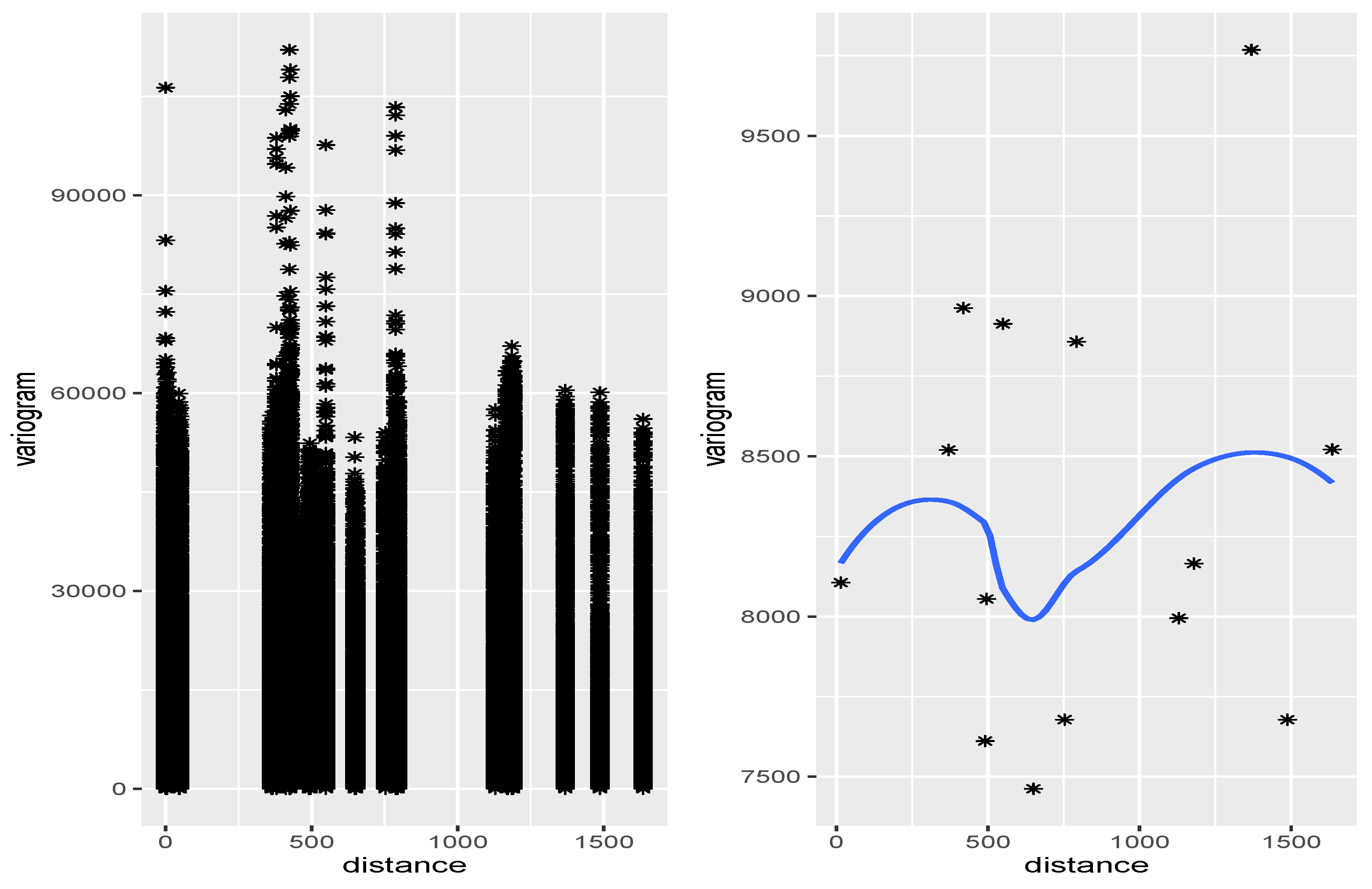
In Figure 3, the left panel shows the variogram cloud for GHI based on eight stations. The right panel shows the empirical variogram, the plot of averaged points of X and Y coordinates of the clouds.
Figure 3.
Variogram cloud (left panel) and an empirical variogram (right panel) for the GHI at the eight radiometric stations. The distance is measured in kilometers.
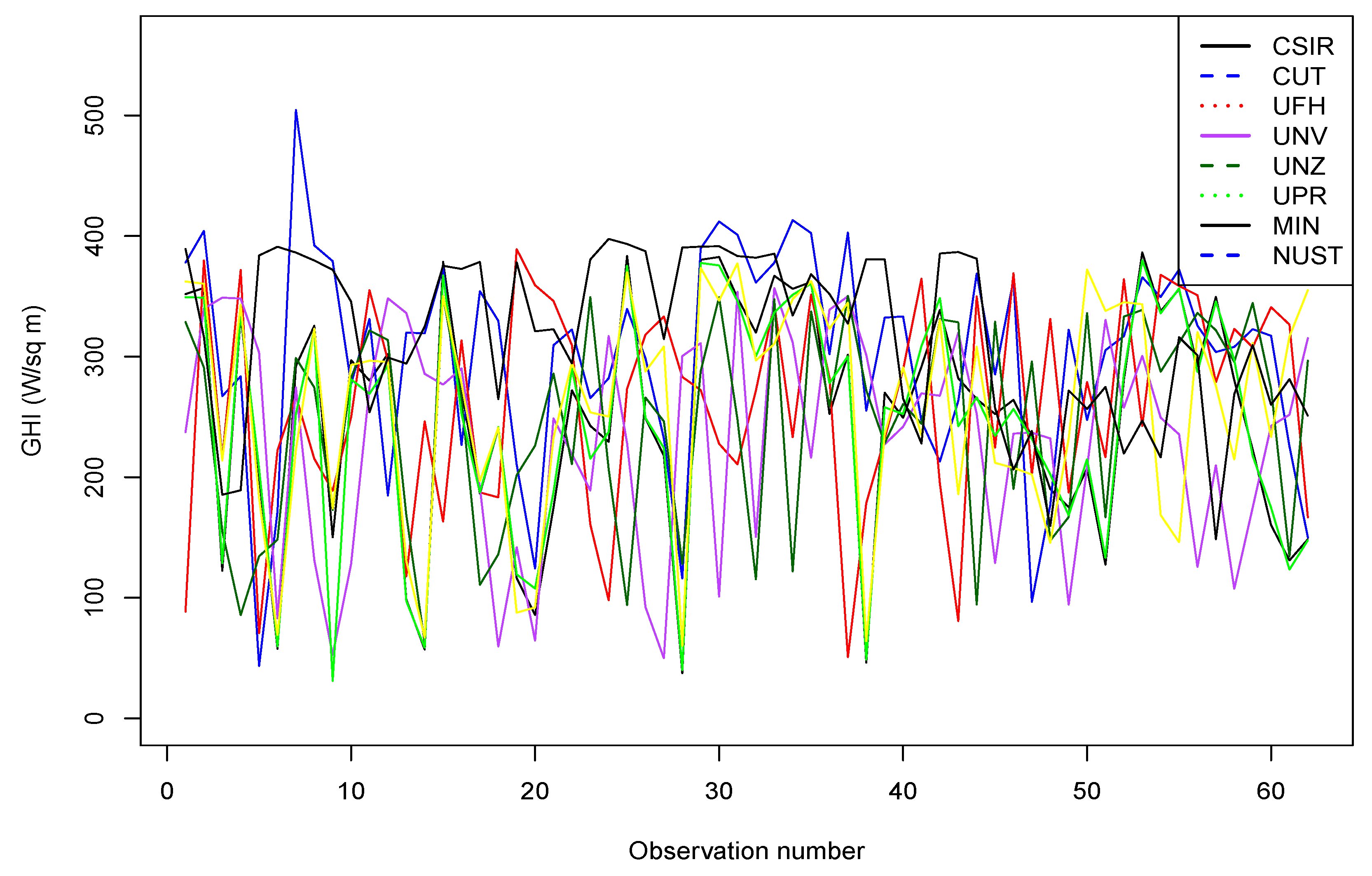
Daily GHI temporal variations of all eight radiometric stations over the sampling period, December 2021 to January 2022, are given in Figure 4. GHI dropped slightly in January compared to December for all the radiometric stations. This is possibly due to the onset of the rainy season.
Figure 4.
Time series plot of the GHI data at the eight radiometric stations.
In order to get some insight into the distribution of the GHI data, the box plots of daily GHI data based on eight radiometric stations are presented in Figure 5. Most stations have GHI values ranging between 20 and 400 W/m. Only CUT and NUST have measures ranging from 100 to 400 and 500 W/m. The spread of the distributions is almost similar except for CUT and NUST, whose spread is slightly different.
Figure 5.
Box plots of GHI at the eight radiometric stations.
Summary statistics of the GHI data are shown in Table 4. The data distribution does not resemble a normal probability distribution since the median and mean are unequal for all eight stations. The measures of skewness are negative, indicating the data are skewed to the left, and kurtosis is less than three for all the stations except CUT, whose kurtosis is greater than three, indicating that its distribution is heavy-tailed.
Table 4.
Summary statistics of GHI for the eight stations.
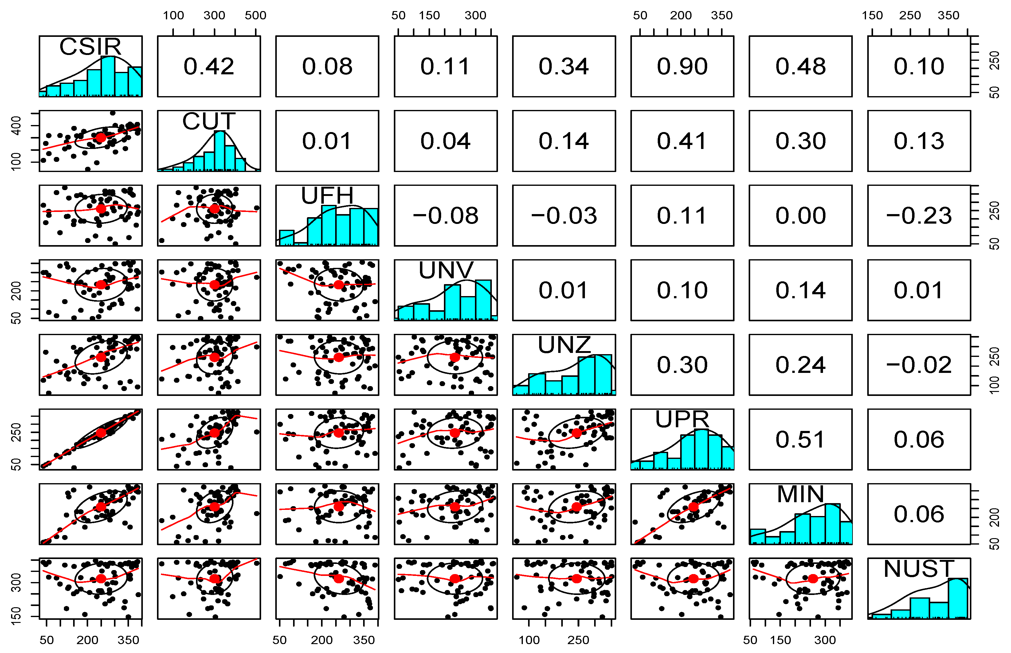
Figure 6 displays the Kendall tau’s coefficients, pairwise scatter plots, and histograms to show the association between the meteorological stations. A measurement of Kendall’s was calculated using Equation (28).
Figure 6.
Histograms (diagonal), pairwise scatter plots (bottom left), and pairwise Kendall’s rank correlation coefficients (top right) of GHI for all the eight radiometric stations.
Measure of indicates weak association, -medium association and fairly strong association and strong association. Most of the associations between stations reflected that most of these stations have strong associations. NUST has a fairly strong negative association with UFH, while CUT and NUST have a positive medium association.
3.3. Variable Selection
In the study, we used ElaticNet, which is one of the shrinkage methods used in variable selection. ElaticNet is a supervised learning algorithm that identifies the variables strongly associated with the dependent variable. The nonlinear rend variable is another important variable that resulted in a significant improvement in the forecast accuracy.
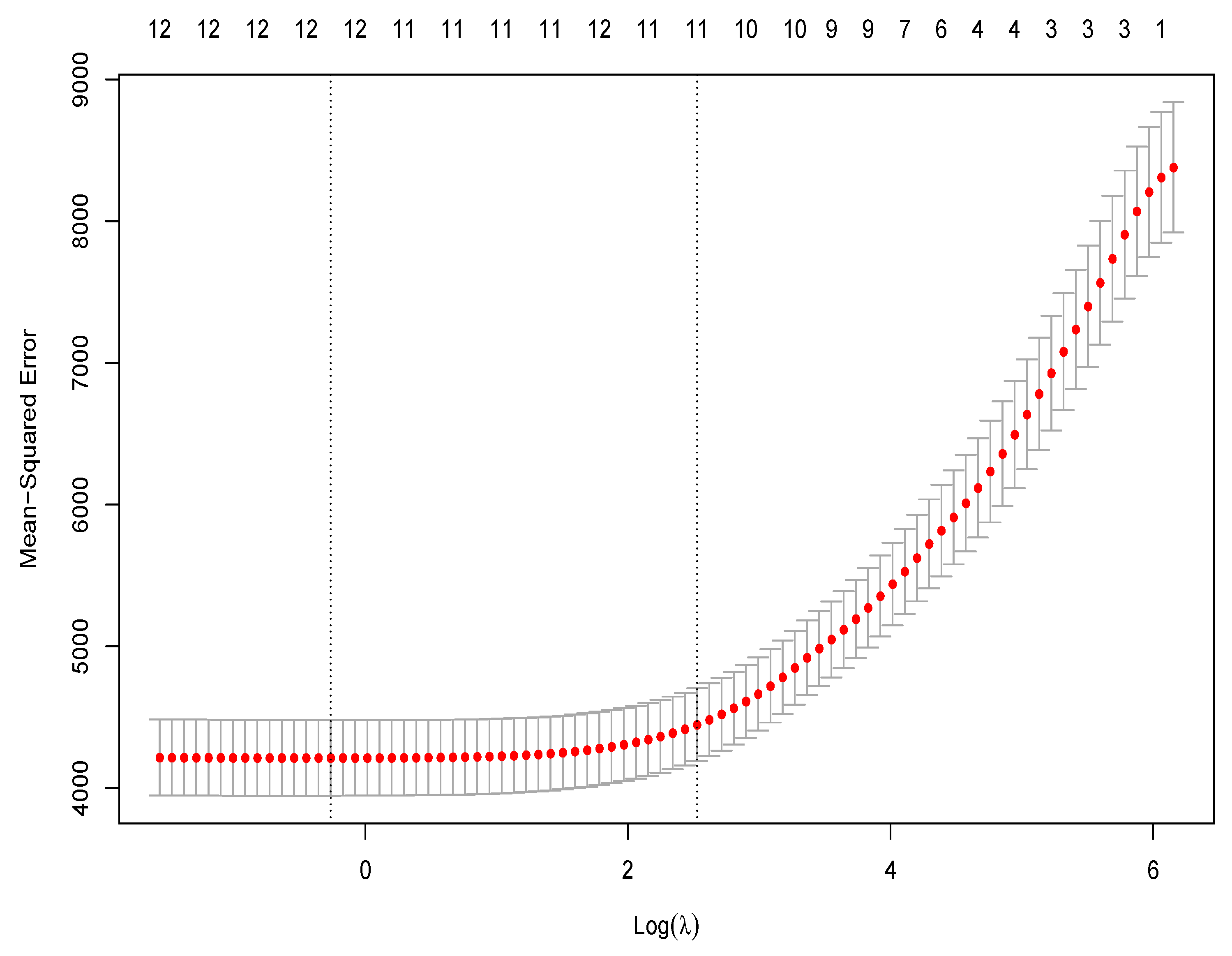
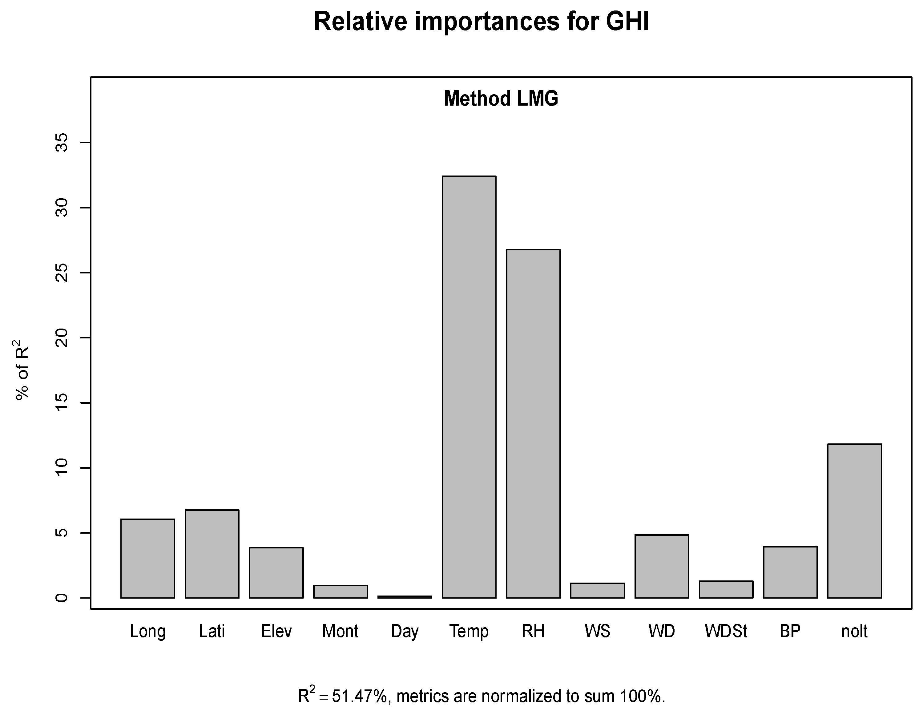
Figure 7 shows the results for variable selection using the R package `glmnet’, [30]. The significance of the variables was checked using the shrinkage method, elastic net. As shown in Figure 7, all twelve variables were retained in the model. Figure 8 shows the relative importance of the independent selected variables. Relative humidity and temperature are the most significant, while the day is the least important covariate.
Figure 7.
Variables selected using the elastic net.
Figure 8.
Relative importance for GHI.
3.4. Forecasting Results
The models used in this study are the linear spatial model (M1), which is the benchmark model, GP spatial regression (M2) and GP spatial autoregressive (M3). Eight radiometric stations were selected, and two months of data were used for each station. Table 5 shows the model evaluations of the forecasting accuracy based on RMSE, MAE, CRPS, and CP. Five stations were used as training sets, and three were used as test sets. With eight stations, the possible number of validation sets is given as , where n is the total number of locations and k is the number of locations in a validation set. In this study, five validation sets, each having three locations, were used.
Table 5.
Overall model evaluation for the three models.
The running times for the three models were as follows: M1 (linear model) took 3.39 s, M2 (GP model) took 2.27 s, and M3 (GP-AR model) took 2.89 s.
The results show that, overall, the spatio-temporal Gaussian regression model (M2) produces the least measures of error based on the MAE and RMSE values, proving to be the best model. Based on the CRPS, the linear spatio-temporal model (M1) is the best-fitting model. However, regarding coverage probability, M1 has the least values on all five validation sets. Overall, M2 is the best-fitting model based on all four evaluation metrics.
We also tested for the statistical significance of the models using the Diebold–Mariano and Giacomini–White tests to check the predictive accuracies of the developed models. The results are given in Table 6. The results show that Model M2 (Gaussian Process Spatial) performed better than all the other models.
Table 6.
Model comparisons (M1(Linear), M2(GP), M3(GP-AR)) using validation set CSIR, UNZ, and NUST.
Figure 9 displays a plot of the forecasts in red and the actual GHI in black. The plots are quite close to each other. We used validation set 2 (CUT, UNV, UPR). The rest of the plots are in the Appendix A section.
Figure 9.
Predictions at CUT, UNV, and UPR radiometric stations.
Kendall’s rank correlation coefficients were used to measure the association between the prediction errors shown in Figure 10. It shows pairwise scatter plots, the Kendall tau coefficients and the histograms. The computations of the Kendall tau coefficients show that errors for stations CUT, UNV and UPR are close to zero except between CUT and UPR, which is 0.17.
Figure 10.
Histograms (diagonal), pairwise scatter plots (bottom left), and pairwise Kendall’s rank correlation coefficients (top right) of the prediction errors for stations 2, 4 and 6, which are CUT, UNV and UPR.
3.5. Standardizing Forecasts
To evaluate the forecasts’ accuracy, we standardized them and then added them back to them. Standardization creates consistency in the dataset by avoiding wider ranges of the predicted values from the actual values.
Table 7 compares the RMSE, MAE, Skill Score, DM, and GW scores, of the predicted values versus the standardized forecasts for validation set UNV, UPR and MIN. The models with standardized predictions achieved better forecasting accuracy, as shown by the positive skill scores. The skill scores show that the predictions improved after standardization.
Table 7.
Standardized based models evaluation.
3.6. Combining Forecasts
Whilst the forecast combination using MCQRNN was applied to all the forecasts from the five validation sets, we present the results from validation set 5 (UNV, UPR, MIN) here. Figure 11 shows plots of combined forecasts with GHI.
Figure 11.
Plots of GHI with forecasts from (a) GP, (b) GP adjusted (c), AR (d) Linear models and combined forecasts using (e) MCQRNN and (f) QGAM.
Table 8 shows forecast evaluations of all the models based on the validation set 5, models GP and AR, Linear and Standardized GP. MCQRNN represents the forecasts that were combined using the QMCRNN model. It is noted from Table 8 that adjusting the forecasts through standardization and combining forecasts significantly improves the forecast accuracy.
Table 8.
Accuracy evaluations (Validation set (467)).
To assess the forecasting results, we use two performance evaluation criteria (RMSE and MAE) with three forecasting horizons, 10-, 15-, and 20-day ahead forecasts. The results are presented in TableTable 9. Using the linear model, the smallest RMSEs for the 10-, 15-, and 20-day ahead forecasts were 62.53, 73.78 and 69.15, respectively. Based on the GP model, the smallest RMSEs were 50.80, 50.32 and 46.10, respectively. Similarly, using the GP-AR model, the RMSEs are 52.96, 51.09 and 45.79, respectively. Based on this validation set and using the RMSE, the results suggest that the GP model is the best for the 10- and 15-day ahead forecasts, while the GP-AR produces good forecasts for the 20-day ahead forecast horizon. It should be noted that this conclusion is based on one validation set. However, this confirms that the spatio-temporal GP regression model produces the most accurate forecasts as summarized in Table 5, Table 6 and Table 8, respectively.
Table 9.
Accuracy evaluations for three forecast horizons using validation set UNV, UPR and MIN.
4. Conclusions
This study investigated the spatial–temporal forecasting of global horizontal irradiance data from eight radiometric stations. The data are from SAURAN (https://sauran.ac.za/), accessed on 13 August 2022. This was done through a comparative analysis of two spatio-temporal predictive models, the Gaussian process regression and the autoregressive Gaussian process regression. Variable selection was done using ElaticNet, a hybrid shrinkage method combining Lasso and ridge regressions. The results were compared to the benchmark model, the spatio-temporal linear model. The spatio-temporal GP outperformed the other two models, proving to be the most appropriate model for predicting GHI in South Africa. Most authors (see, for example, [20,31]) applied models based on single-site data sets for predicting solar power irradiation. Accurate forecasts of solar power from multi-sites are important to the system operator, as they facilitate large-scale integration of solar power onto the power grid. This modeling approach exploits production information of solar power from neighboring radiometric stations.
Energy forecasting has many limitations; among them is coming up with accurate forecasts. In order to improve the forecasts, standardization was done, and it proved that the models’ forecasting accuracy improved. The forecasts from the individual models were combined using quantile regression neural networks and additive quantile regression models, which resulted in a significant improvement in the forecast accuracy. As a result, there was a significant improvement in forecast accuracy. This modeling framework could be useful to power utility companies in making informed decisions when planning power grid management.
This study has several possible future research directions. The modeling done in the current paper involved stations in geographically sparse areas. Future research could use more stations and cluster them before the spatio-temporal forecasting of solar power. An in-depth analysis of the extremal dependence of GHI in each cluster could help develop models with high predictive capabilities. Another interesting research could be using large data sets from stations at different periods and comparing them with those from gridded data sets.
Author Contributions
Conceptualization, E.C. and C.S.; methodology, E.C. and C.S.; software, E.C.; validation, E.C. and C.S.; formal analysis, E.C.; investigation, E.C.; data curation, E.C. and C.S.; writing—original draft preparation, E.C.; writing—review and editing, E.C., C.S. and A.B.; visualisation, E.C. and C.S.; supervision, C.S. and A.B.; project administration, C.S. and A.B. All authors have read and agreed to the published version of the manuscript.
Funding
This research received no external funding.
Institutional Review Board Statement
Not applicable.
Informed Consent Statement
Not applicable.
Data Availability Statement
The data used in this study are from Southern African Universities Radiometric Network (SAURAN), website (https://sauran.ac.za/, accessed on 13 August 2022). The analytic data can be downloaded from https://github.com/csigauke/Data-for-the-article-Spatio-temporal-forecasting-of-global-horizontal-irradiance-using-Bayesian-inf.
Acknowledgments
The authors acknowledge SAURAN, Southern African Universities Radiometric Network, for providing the data.
Conflicts of Interest
The authors declare no conflict of interest.
Abbreviations
The following abbreviations are used in this manuscript:
| GHI | Global horizontal irradiance |
| GP | Gaussian Process |
| GP Spatial | Gaussian Process Spatial Regression |
| GP ARSpatial | Gaussian Process Autoregressive Spatial Model |
| LSTR | Linear Spatial Temporal Regression |
| ARX | autoregressive with exogenous inputs |
| NN | Neural Network |
| RRF | random regression forest |
| RT | regression trees |
| ANN | Artificial Neural Network |
| SVR | Support Vector Regression |
| ARIMAX | Autoregressive Moving Average |
| DNN | Deep Neural Network |
| MLP | artificial neural networks |
| MGGP | multigene genetic programming |
| RSME | Root Mean Square Error |
| MAE | Mean absolute error |
| CPRS | Continuous Ranked Probability Score |
| CP | Prediction Interval Coverage |
| SAURAN | Southern African Universities Radiometric Network |
| MDPI | Multidisciplinary Digital Publishing Institute |
| CSIR | CSIR Energy Centre |
| CUT | Central University of technology |
| UFH | University of Fort Hare |
| UNV | university of Venda |
| UNZ | University of Zululand |
| UPR | University of Pretoria |
| MIN | CRSES Mintek |
| NUST | Namibian University of Science and Technology |
| QGAM | Quantile Generalized Additive Model |
| MCQRNN | Monotone Composite Quantile Regression Neural Networks |
Appendix A
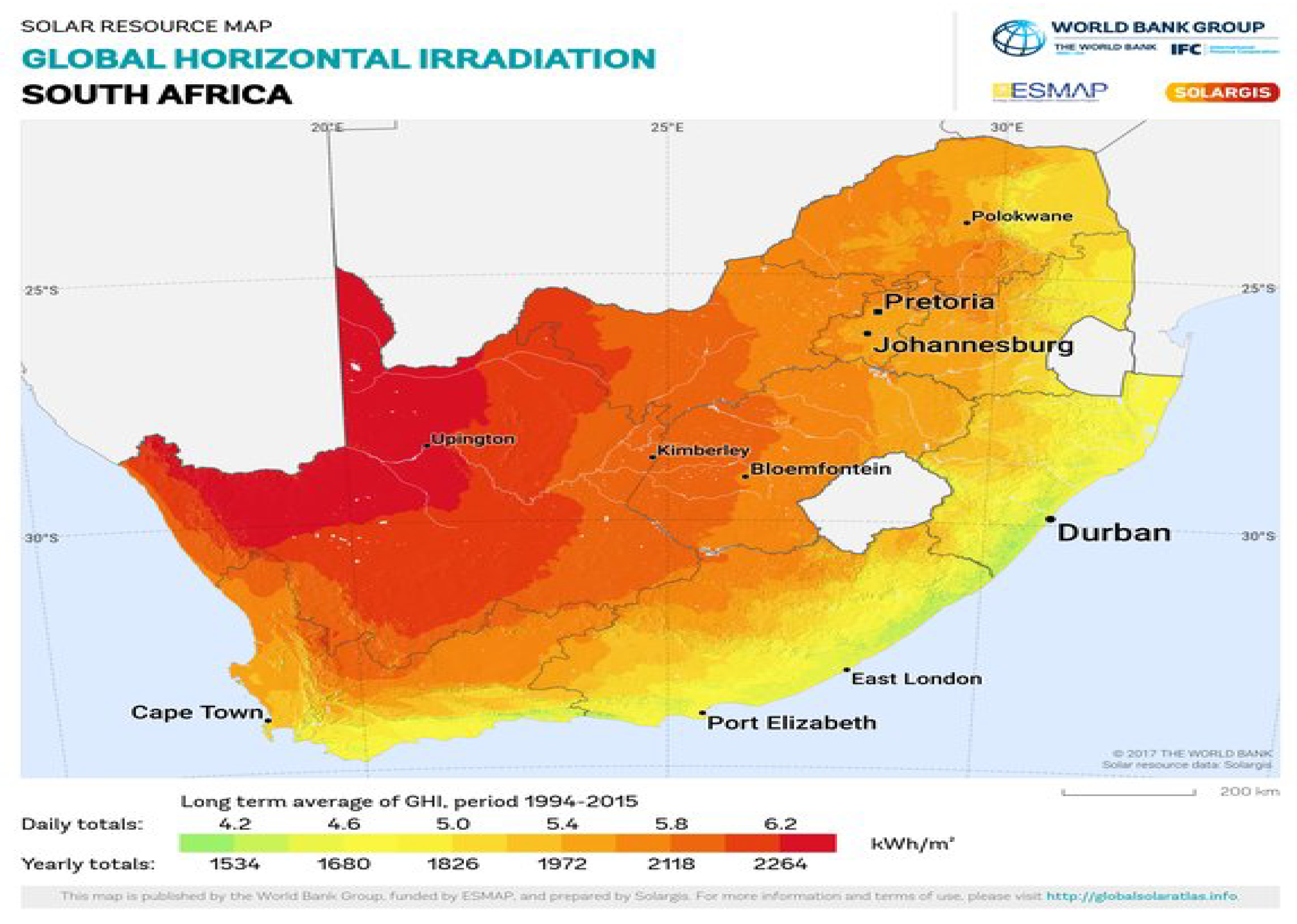
Figure A1 shows the solar resource map for South Africa (SA). It shows the solar radiation each area (region) in SA receives. The largest amount of GHI is in the western part of South Africa.
Figure A1.
Solar heat map. Source: https://solargis.com/maps-and-gis-data/download/south-africa, accessed on 8 July 2022.
References
- Hong, T.; Shahidehpour, M. Load Forecasting Case Study; US Department of Energy: Washington, DC, USA, 2015. [Google Scholar]
- Andre, M.; Dabo-Niang, S.; Soubdhan, T.; Ould-Baba, H. Predictive -temporal model for spatially sparse global solar radiation data. Energy 2016, 111, 599–608. [Google Scholar] [CrossRef]
- Liu, Y.; Qin, H.; Zhang, Z.; Pei, S.; Wang, C.; Yu, X.; Jiang, Z.; Zhou, J. Ensemble temporal forecasting of solar irradiation using variational Bayesian convolutional gate recurrent unit network. Appl. Energy 2019, 253, 113596. [Google Scholar] [CrossRef]
- Yang, D. Ultra-fast pre-selection in lasso-type -temporal solar forecasting problems. Sol. Energy 2018, 176, 788–796. [Google Scholar] [CrossRef]
- Eschenbach, A.; Yepes, G.; Tenllado, C.; G<i>o</i>´mez-P<i>e</i>´rez, J.I.; Pi<i>n</i>˜uel, L.; Zarzalejo, L.F.; Wilbert, S. Spatio-Temporal Resolution of Irradiance Samples in Machine Learning Approaches for Irradiance Forecasting. IEEE Acess 2020, 8, 51518–51531. [Google Scholar] [CrossRef]
- Kim, B.; Suh, D. A Hybrid -Temporal Prediction Model for Solar Photovoltaic Generation Using Numerical Weather Data and Satellite Images. Remote Sens. 2020, 12, 3706. [Google Scholar] [CrossRef]
- Zhang, J.; Ju, Y.; Mu, B.; Zhong, R.; Chen, T. An efficient implementation for spatial–temporal Gaussian process regression and its applications. Automatica 2023, 147, 110679. [Google Scholar] [CrossRef]
- Todescato, M.; Carron, A.; Carli, R.; Pillonetto, G.; Schenato, L. Efficient spatio-temporal Gaussian regression via Kalman filtering. Automatica 2022, 118, 109032. [Google Scholar] [CrossRef]
- Hamelijnck, O.; Wilkinson, W.; Loppi, N.; Solin, A.; Damoulas, T. Spatio-temporal variational Gaussian processes. Adv. Neural Inf. Process. Syst. 2021, 2021 34, 23621–23633. [Google Scholar]
- Agoua, X.G.; Girard, R.; Kariniotakis, G. Probabilistic models for spatio-temporal photovoltaic power forecasting. IEEE Trans. Sustain. Energy 2018, 10, 780–789. [Google Scholar] [CrossRef]
- Banerjee, S.; Gelfand, A.E.; Finley, A.O.; Sang, H. Gaussian predictive process models for large spatial data sets. J. R. Stat. Soc. Ser. B (Stat. Methodol.) 2008, 70, 825–848. [Google Scholar] [CrossRef]
- Luttinen, J.; Ilin, A. Variational Gaussian-process factor analysis for modeling spatio-temporal data. Adv. Neural Inf. Process. Syst. 2009, 22. Available online: https://proceedings.neurips.cc/paper/2009/file/4a47d2983c8bd392b120b627e0e1cab4-Paper.pdf (accessed on 19 September 2022).
- Tomizawa, Y.; Yoshida, I. Benchmarking of Gaussian Process Regression with Multiple Random Fields for Spatial Variability Estimation. ASCE-ASME J. Risk Uncertain. Eng. Syst. Part A Civ. Eng. 2022, 8, 04022052. [Google Scholar] [CrossRef]
- Comber, A.; Harris, P.; Brunsdon, C. Spatially Varying Coefficient Regression with GAM Gaussian Process splines: GAM (e)-on. AGILE GISci. Ser. 2022, 2022 3, 1–6. [Google Scholar] [CrossRef]
- Najibi, F.; Apostolopoulou, D.; Alonso, E. Enhanced performance Gaussian process regression for probabilistic short-term solar output forecast. Int. J. Electr. Power Energy Syst. 2021, 130, 106916. [Google Scholar] [CrossRef]
- Najibi, F.; Apostolopoulou, D.; Alonso, E. Clustering Sensitivity Analysis for Gaussian Process Regression Based Solar Output Forecast. IEEE Madr. PowerTech 2021, 1–6. [Google Scholar] [CrossRef]
- de Paiva, G.M.; Pimentel, S.P.; Alvarenga, B.P.; Marra, E.G.; Mussetta, M.; Leva, S. Multiple Site Intraday Solar Irradiance Forecasting by Machine Learning Algorithms: MGGP and MLP Neural Networks. Energies 2020, 13, 3005. [Google Scholar] [CrossRef]
- Wang, F.; Chen, P.; Zhen, Z.; Yin, R.; Cao, C.; Zhang, Y.; Duic, N. Dynamic -temporal correlation and hierarchical directed graph structure based ultra-short-term wind farm cluster power forecasting method. Appl. Energy 2022, 323, 119579. [Google Scholar] [CrossRef]
- Gill, J.; Rubiera, J.; Martin, C.; Cacic, I.; Mylne, K.; Dehui, C.; Jiafeng, G.; Xu, T.; Yamaguchi, M.; Foamouhoue, K.; et al. Guidelines on Communicating for Uncertainty; World Meteorological Organisation: Geneva, Switzerland, 2008; Available online: https://public.wmo.int/en (accessed on 6 July 2022).
- Chandiwana, E.; Sigauke, C.; Bere, A. Twenty-four-hour ahead probabilistic global horizontal irradiance forecasting using Gaussian process regression. Algorithms 2021, 14, 177. [Google Scholar] [CrossRef]
- Zou, H.; Hastie, T. Regularization and variable selection via the elastic net. J. R. Stat. Soc. Ser. B (Stat. Methodol.) 2005, 67, 301–320. [Google Scholar] [CrossRef]
- Williams, C.K.I.; Rasmussen, C.E. Gaussian processes for machine learning. Cambridge 2006, 2, 69–106. [Google Scholar]
- Sahu, S.K. Bayesian Modeling of Spatio-Temporal Data with R, 1st ed.; CRC Press/Taylor and Francis: New York, NY, USA, 2022. [Google Scholar]
- Zou, H.; Yuan, M. Composite quantile regression and the oracle model selection theory. Ann. Stat. 2008, 36, 1108–1126. [Google Scholar] [CrossRef]
- Jin, J.; Zhao, Z. Composite Quantile Regression Neural Network for Massive Datasets. Math. Probl. Eng. 2021, 1–10. [Google Scholar] [CrossRef]
- Fasiolo, M.; Wood, S.N.; Zaffran, M.; Nedellec, R.; Goude, Y. QGAM: Bayesian Nonparametric Quantile Regression Modeling in R. J. Stat. Softw. 2021, 100, 1–31. [Google Scholar] [CrossRef]
- Diebold, F.X.; Mariano, R.S. Comparing predictive accuracy. J. Bus. Econ. Stat. 2002, 20, 134–144. [Google Scholar] [CrossRef]
- Triacca, U. Comparing Predictive Accuracy of Two Forecasts. 2018. Available online: http://www.phdeconomics.sssup.it/documents/Lesson19.pdf (accessed on 7 September 2022).
- Giacomini, R.; White, H. Tests of conditional predictive ability. Econometrica 2006, 74, 1545–1578. [Google Scholar] [CrossRef]
- Hastie, T.; Qian, J.; Tay, K. An Introduction to Glmnet. Available online: https://cran.r-project.org/web/packages/glmnet/vignettes/glmnet.pdf (accessed on 23 August 2022).
- Sigauke, C.; Ravele, T.; Jhamba, L. Extremal Dependence Modelling of Global Horizontal Irradiance with Temperature and Humidity: An Application Using South African Data. Energies 2022, 15, 5965. [Google Scholar] [CrossRef]
Disclaimer/Publisher’s Note: The statements, opinions and data contained in all publications are solely those of the individual author(s) and contributor(s) and not of MDPI and/or the editor(s). MDPI and/or the editor(s) disclaim responsibility for any injury to people or property resulting from any ideas, methods, instructions or products referred to in the content. |
© 2022 by the authors. Licensee MDPI, Basel, Switzerland. This article is an open access article distributed under the terms and conditions of the Creative Commons Attribution (CC BY) license (https://creativecommons.org/licenses/by/4.0/).