Article

Low-Quality Integrated Circuits Image Verification Based on Low-Rank Subspace Clustering with High-Frequency Texture Components

1
School of Integrated Circuits, Guangdong University of Technology, Guangzhou 510006, China
2
School of Automation, Guangdong University of Technology, Guangzhou 510006, China
3
The Fifth Electronics Research Institute of the Ministry of Industry and Information Technology of China, Guangzhou 510630, China
4
Guangdong Provincial Key Laboratory of Electronic Information Products Reliability Technology, Guangzhou 511370, China
5
Neuroeconomics Laboratory, Guangzhou Huashang College, Guangzhou 511399, China
*
Authors to whom correspondence should be addressed.
Appl. Sci. 2023, 13(1), 155; https://doi.org/10.3390/app13010155
Submission received: 16 November 2022 / Revised: 7 December 2022 / Accepted: 19 December 2022 / Published: 22 December 2022
(This article belongs to the Special Issue Visual Inspection Using Machine Learning and Artificial Intelligence)

Abstract

:
With the vigorous development of integrated circuit (IC) manufacturing, the harmfulness of defects and hardware Trojans is also rising. Therefore, chip verification becomes more and more important. At present, the accuracy of most existing chip verification methods depends on high-precision sample data of ICs. Paradoxically, it is more challenging to invent an efficient algorithm for high-precision noiseless data. Thus, we recently proposed a fusion clustering framework based on low-quality chip images named High-Frequency Low-Rank Subspace Clustering (HFLRSC), which can provide the data foundation for the verification task by effectively clustering those noisy and low-resolution partial images of multiple target ICs into the correct categories. The first step of the framework is to extract high-frequency texture components. Subsequently, the extracted texture components will be integrated into subspace learning so that the algorithm can not only learn the low-rank space but also retain high-frequency information with texture characteristics. In comparison with the benchmark and state-of-the-art method, the presented approach can more effectively process simulation low-quality IC images and achieve better performance.

1. Introduction

Machine learning and the integrated circuit (IC) manufacturing industry have advanced rapidly in the last decade. The expansion of the IC industry especially has led to a new pursuit of efficiency in all aspects. Verification is one of the core steps in the chip design and production process, so traditional inspection methods needed to be replaced by new automated inspection means urgently. Therefore, efficient verification techniques based on computer vision or machine learning algorithms have received a lot of attention in recent years [1,2,3,4]. In the proposed process of such verification techniques, their validity is mostly derived from the high-quality ICs’ images being utilized as a test set. The goal of this paper is to suggest an algorithm for the effective classification of low-quality ICs’ images in order to reduce the stringent requirements on samples and provide a reliable, valid, and easily accessible database for the subsequent verification procedures.
With annual semiconductor sales exceeding USD 400 billion for the first time in 2018 [5], the need for reliability verification in the semiconductor industry has reached a new pinnacle, and there are two common types of defect objects in reliability verification, which are unintentional defects and malicious hardware Trojans (HTs). Unintentional defects can be caused by immature processes that result in low yields or poor processing environments, such as solder joint offsets and stained spots. These defects are not the original design intent, so they can be solved by improving the process and production environment. In contrast, HTs are human-implanted and can exist in two important stages of IC production, including design and manufacturing. Even more problematic is the fact that today’s IC production is a global collaborative model, with various stages of the industry scattered around the globe, making it easy for HTs to break in. HTs can leak secret information, disable ICs, or cause other catastrophic consequences [6,7,8]. In 2009, a statistical approach was proposed with the idea of constructing a series of fingerprints based on the path delay of gold chips to verify whether the chips contain HTs by comparing the delay parameters of the chips with the fingerprints [9]. With the booming development of computer vision, vision-based techniques are one of the hot research topics in the last decade. A machine learning algorithm based on power analysis was proposed in [10], which aims to obtain the hardware Trojan infection algorithm and use machine learning to detect hardware Trojan implantation. One HT classification method is called Hardware Trojan Learning Analysis (ATLAS) [11], which identifies HT-infected circuits using a gradient boosting (GB) model on data from the gate-level netlist (GLN) stage. A method is proposed to extract the basic features of digital circuits using Haar features and augment their features with the AdaBoost learning algorithm to generate strong classifiers [12]. Two hardware Trojan detection algorithms based on support vector machine (SVM)-supervised machine learning were designed [13,14]. In [15], the intrinsic nature of many cores providing feedback to the online learning algorithm based on the core information and its behavior with incoming packets was designed for a real-time online learning method. As a latecomer, deep learning has also made a lot of achievements in this field in recent years. A deep learning (DL) class of ML was proposed based on extracting the raw circuit features and feeding them into a DL model (deep stacking autoencoder) that extracts the features which contribute to HT detection [16]. A novel, golden, reference-free HT detection method named GNN4TJ [17] was proposed in the register transfer level (RTL) based on a graph neural network (GNN). A deep learning model, GATE Net, based on graph convolutional networks (GCNs), was proposed in [18], which is trained using supervised contrast learning for labeling designs containing random insertion triggers using only the corresponding netlist. A new model-based dynamic convolution neural network (DCNN) architecture was developed in [19], which includes three convolutional and pooling layers for automatically extracting invariant and relevant features from IC images. A new graph learning (GL)-based method for detecting node HTs, called NHTD-GL, was proposed in [20].
As more and more companies join the chip manufacturing sector, the need for flow and verification of chip designs after they are completed is also on the rise. However, unlike large companies, which have the financial resources to spend large sums of money on scanning electron microscopes (SEMs) to facilitate the subsequent verification process, small- and medium-sized companies are forced to outsource this step to professional facilities, albeit at a high cost. In essence, this is because the availability of validation tools is based on high-quality IC images. This creates a contradiction: the high difficulty of obtaining high-quality images and the indispensability of noiseless high-quality IC images. This contradiction is also one of the biggest obstacles between academia and industry. A low-cost and easily achievable alternative is, therefore, worth exploring.
The aim of this paper is to propose an algorithm for the recovery of low-quality image information for subsequent detection tasks. As the approach is pragmatic, the data used in the experiments will take into account the following practices and common situations:
(1)
Unlike SEM, which uses a narrowly focused high-energy electron beam to scan the sample and sweep the image elements from left to right and from top to bottom on a sample to obtain a high-precision, full-range image in a single pass, the workflow of a normal camera with a microscope is still to capture different partial views several times and finally combine them into a complete large image.
(2)
For the sensor on the camera, the unstable temperature and light source of the acquisition environment can bring about changes in the signal-to-noise ratio (SNR), and images with low SNRs often contain a variety of noises.
(3)
Image data may be corrupted when uploading from the camera to the server, such as due to multiplicative noise caused by unsatisfactory channels.
To cope with the images obtained in the above scenario, this paper proposes a fused representation clustering framework called High-Frequency Low-Rank Subspace Clustering (HFLRSC), where high frequency means the High-Frequency Texture Component (HFTC). In HFLRSC, A fused subspace learning framework that incorporates an HFTC and low-rank constraints is proposed. Experiments on simulated data show that the method can effectively process low-quality IC images and achieve better performance than the benchmark and existing methods.

2. Background Knowledge

This section will briefly introduce the related background knowledge on low-rank representation learning and the high-frequency texture component.

2.1. Low-Rank Representation

Due to the problem of the signal-to-noise ratio, the current data acquisition methods will inevitably cause varying degrees of noise pollution in the datasets. To reconstruct a low-rank matrix from polluted data, LRR was developed. Given a dataset X that has been polluted by errors P , X can be thought of as a mixture of two parts ( X = U + P ), where the raw data U should be of a low rank. In order to achieve the above objectives, the subsequent regularization rank minimization equation could be formulated as
min U , P r a n k ( U ) + λ P l s . t . X = U + P ,
where λ is a trade-off parameter and · l also indicates a specific regularization technique for the error term.
After introducing an extra dictionary matrix, the more general rank minimization problem can be applied to more real mixed data as follows:
min C , P r a n k ( C ) + λ P l s . t . X = UC + P ,
where U is a dictionary. Under the circumstances, the minimum solution of C which can be abbreviated as C * is the “lowest rank representation” of X. In the process of practical application, it is difficult to build an appropriate dictionary. Therefore, the self-representation method of using itself [21] as a dictionary came into being. At this time, C * represents the sample’s subspace knowledge and can be used for clustering.

2.2. High-Frequency Texture Component

In general, there are two important components constructing the information of the image: a texture component and a structure component. The morphological information of an image is represented by the texture component, while the structure component represents the structure. Therefore, the essential characteristic of the image can be revealed well by the texture component. The texture component knowledge can be useful for rebuilding images using compressive sensing algorithms.
The image texture component is the high-frequency information, which is easy to achieve. Among our pretests, we successfully propose an effective method to extract the morphological characteristic of human face images and utilize it to distinguish different individuals. In the IC image, the key information is the shapes, layouts, and wiring of its electronic components. The edges of elements will create the pixel change regions in the images, which can also be effectively captured and extracted by the high-pass filter, and the high-pass filter can effectively capture and extract the pixel change region generated by the edges of electronic components. Even if the resolution of IC images is low and full of noise, the features extracted by HFTC are still enough for classification and the following procedures.

3. The Proposed Approach

The motivation and architecture of HFLRSC will be discussed in detail in this section.

3.1. Proposed Framework

In just about all instances, conventional clustering approaches would consider all of the data’s knowledge during the procedure, which is effective for noiseless data. However, data in the real world are often noised, and the noise may be non-sparse or of a high intensity. The noise may form some pixel blocks in the samples and cause those samples to lose their features. Thus, traditional methods would probably categorize those noised samples into the same cluster. Inspired by our pretests, the HFTC features extracted from face images can maintain valuable morphological information well and greatly weaken the noise, we believe that HFTC extraction can make better use of the key knowledge of low-quality IC images. To be specific, the valuable information of the ICs’ images exists in the layout and wiring of the electronic components in the field of IC defect detection (visual detection methods). While the layout and wiring can be effectively retained by HFTC extraction. In the meantime, the impact of environmental noise and pixel loss will be significantly reduced in the extraction process, which is very conducive to the subsequent clustering tasks.
In machine learning tasks, each individual sample in the dataset is usually assembled into a column as X = x i | i = 1 , , N . Each individual sample, designated by the letter x i , must be reshaped during the extraction process to its original height and width, designated by X i . In order to facilitate the following discussion, the height and width of X i are represented by H and W, respectively. Then, X i ^ can be made to represent the expression of data X i in the frequency domain, which is derived by using a two-dimensional Fourier transform (2D FFT):
X i ^ ( s , t ) = m = 1 H n = 1 W x i ( m , n ) e j 2 π ( m s H + n t W ) ,
where ( s , t ) and ( m , n ) denote the coordinates. Then, the high-frequency texture components of the images h 1 ^ , , h n ^ are obtained by using a high-pass filter H to process frequency domain data and apply an inverse two-dimensional FFT to the filtered frequency domain data:
h i ^ ( m , n ) = 1 H 1 W s = 1 H t = 1 W H X i ^ ( m , n ) e j 2 π ( m s H + n t W ) .
Then, h i ^ is restructured as a column vector h i and combined to form the matrix H = { h 1 , , h N } R d × n .
The high-frequency texture components retain most morphological information, which can reveal the essential details for better distinguishing individuals. When the data are noised, the traditional clustering methods may not work as usual, particularly when the noise is not sparse and has a high energy level. Using IC images as examples, when distinct circuit images are obscured by Gaussian noise or flaws, they may be classified as part of the same cluster because of the high energy of the covers. The noise described above is low-frequency information that can be considerably decreased following HFTC extraction, from which it can be concluded that using an HFTC will assist representation learning and increase subsequent clustering performance.
Rather than sharing an entire uniform space, the samples of dataset X are typically located in their distinct low-dimensional subspaces. The LRR problem [22] can be reformulated using the self-representation method:
min C r a n k ( C ) + λ XC X l
where | | XC X l represents the sparse error measurement. Using the knowledge of the high-frequency texture component matrix H and a Frobenius norm to estimate the error between the texture component and the original data, the LRR formula can be reformulated as follows:
min C r a n k ( C ) + λ 1 XC H F 2 + λ 2 XC X l
where λ 1 and λ 2 are the trade-off parameters. In the iterative process, the algorithm can learn the unique representation of C by integrating all aspects of the knowledge. Since the rank (·) operator is a non-convex problem, a convex kernel norm is typically used to relax it [23]. As a matter of convenience, P can be used to represent the data’s own error term. Finally, High-Frequency Low-Rank Subspace Clustering (HFLRSC) is proposed, which is written as a minimization problem:
min C , P C * + λ 1 XC H F 2 + λ 2 P l s . t . X = XC + P
As previously described, λ 1 and λ 2 are the trade-off parameters. The nuclear norm and the Frobenius norm are denoted by · * and · F , respectively. Within this framework, the · F function is used to estimate the distance between the self-representation term XC and the texture component term H . Subspace C will progressively acquire the information stored in the texture components during the iterative procedure of minimizing the term XC H F 2 . Because of the sparse error and low-rank term limitations, the learning results will attain a relative balance while modifying the trade-off parameters.
When C is obtained, the category to which each sample belongs can be revealed by the subspace structure. With C , the affinity matrix could be generated as follows:
W = | C | + | C T | 2
where | · | is the absolute operator. The final clustering results can be acquired using the standard Special Clustering (SC) approach by using the generated w matrix as illustrated below:
min F T r ( F T LF ) s . t . F T DF = I
where T r ( · ) denotes the trace of the matrix. F denotes the cluster indicator matrix, while I denotes the identity matrix. L is the Laplacian matrix, and D is a diagonal matrix whose elements are the sum of the ith row or ith column of W. Thus, Equation (9) can be effectively transformed into an eigenvalue decomposition problem, and the clustering index of the data points can be directly expressed by a matrix F .

3.2. Solution to HFLRSC

This section will provide a brief overview of the HFLRSC solution and essential steps. The optimization problem in Equation (7) is convex and can be solved by various methods. For efficiency, we adopt in this paper the Augmented Lagrange Multiplier (ALM) [24] method. We first convert Equation (7) to the following equivalent problem:
min C , R , P C * + λ 1 XR H F 2 + λ 2 Ω ( P ) s . t . X = XR + P , R = C
The problem can be solved by the ALM method, and the objective function using the ALM method can be written as
L = C * + λ 1 XR H F 2 + λ 2 Ω ( P ) + μ 2 XR + P X + β 1 μ F 2 + C R + β 2 μ F 2
The above problem is unconstrained. Thus, it can be minimized with respect to C , R , and P by fixing the other variables and then updating the Lagrange multipliers β 1 and β 2 , where μ > 0 is a penalty parameter. The inexact ALM method, also called the alternating direction method, is used in HFLRSC and is outlined in Algorithm 1.
In Algorithm 1, the subscript t indicates the index of iteration. Θ ( a , b ) = U S b ( Σ a ) V T is the singular value thresholding (SVT) operator, in which U Σ a V T is the singular value decomposition (SVD) of a and S b ( X ) = S i g n ( X ) m a x ( | X | q , 0 ) is the soft threshold operator.
Algorithm 1: The algorithm of HFLRSC.
Applsci 13 00155 i001

4. Experimental Study

In this section, we conduct extensive experiments on simulation datasets to verify the effectiveness of the proposed approach. All experimental data were obtained from a real-world scanning electron microscope at different settings.

4.1. Data Preparation

In the implementation, we chose to use simulated samples obtained by processing high-quality images from the real world due to several reasons. First of all, it is hard to access sufficient quantities of the desired low-resolution equipment. Secondly, the high-quality image used in this experiment was taken by a scanning electron microscope, meaning that it should be able to represent the highest-quality chip image. Therefore, the down-sampling of high-quality images in different proportions is effective for simulating different conditions for low-resolution devices. In addition, the simultaneous interpreting of different sizes and intensities of the image is used to simulate the sizes of different sensors, because the size of the sensor is positively correlated with the signal-to-noise ratio (SNR). Based on the above discussion, we entrusted an authoritative research institution, named the Science and Technology on Reliability Physics and Application of Electronic Component Laboratory, with the high-quality chip images scanned by an electron microscope. Based on the principle of confidentiality of information and the frequency with which the chip was attacked, the research institution provided a real image of the chip. Figure 1 shows a general view of this chip.
There was one more major processing step before we proceeded with the clustering experiment, which was histogram equalization. This method is generally utilized to increase the global contrast of images, especially when the contrast of the valid data of the image is quite close. Through this method, the brightness can be better distributed on the histogram. In the actual production process, it is difficult to obtain timely and high-quality chip images to analyze whether there are hardware Trojans and defects, which are caused by equipment accuracy, environmental interference, and operation error. In order to solve the above shackles, different partial views of the chip can be scanned multiple times through a low-precision lens, and all partial views can be reassembled into a complete chip image.
When obtaining experimental data, the low-quality image would be simulated through the following three steps. First, we divided the full-view pictures into several parts and further controlled the resolution by reducing the sampling proportionally. Secondly, the defects of different sizes and numbers extracted from real chip images were covered on the simulated data samples. Lastly, we added different strengths of Gaussian noise, salt-and-pepper noise, and multiplicative noise to simulate environmental interference. Figure 2 presents a part of the simulated low-quality images of ICs. In this experiment, a complete chip image would be divided into 12 parts, and each part would be divided into 10 categories by adding defective blocks at random locations and the same noise intensity. Therefore, the dataset size of this experiment was 10 categories and 120 samples in total.
Next is the explanation of the noise parameters. “Gaussian 0.1” means adding Gaussian white noise, where the mean value is 0.1 and the variance is 0.01 by default. “Multiplicative noise 0.1” means adding multiplicative noise using equation J = I + n I , where I is the original image and N is the uniformly distributed random noise with a mean value of 0 and variance of 0.1 by default. The range of the mean and variance parameters of Gaussian noise and multiplicative noise types is [0, 1]. “Salt-and-Pepper 0.1” means adding salt and pepper noise, where 0.1 is the noise density, which means it will affect about 0.1 n u m e l ( I ) pixels.

4.2. Comparison Methods

In this experiment, we chose K-means and spectral clustering with normalized cut (Ncut) for the baseline. Classical representation learning algorithms including Sparse Subspace Clustering (SSC) [25] and Low-Rank Representation (LRR) [23] were also adopted for comparison. We also added two recent clustering algorithms for comparison: SC-SRGF [26] and USENC [27].
Next, the five general performance indicators selected in this section are introduced.The accuracy (ACC) was calculated using the Hungarian algorithm to best map among the ground true labels and cluster results. The purity and accuracy in classification problems are similar. It takes the most classes in each cluster to be the class represented by this cluster, calculates the number of correctly allocated classes, and then divides this number by the total to obtain a value. The normalized mutual information (NMI) is used to measure the correlation between data distribution. The higher the mutual information, the higher the correlation. The F-measure (F) is a combination of precision and recall in information retrieval for clustering evaluation. The adjusted Rand index (ARI) indicates the similarity between the two clusters.

4.3. Results and Analyses

In this section, we will conduct clustering of the simulated datasets with different degrees and types of noise under the condition of the same pixel loss. In particular, we fixed the number of defects at 10, which was to simulate the chip with a small number of defects in the general scenario, as too many or too little would appear impractical.
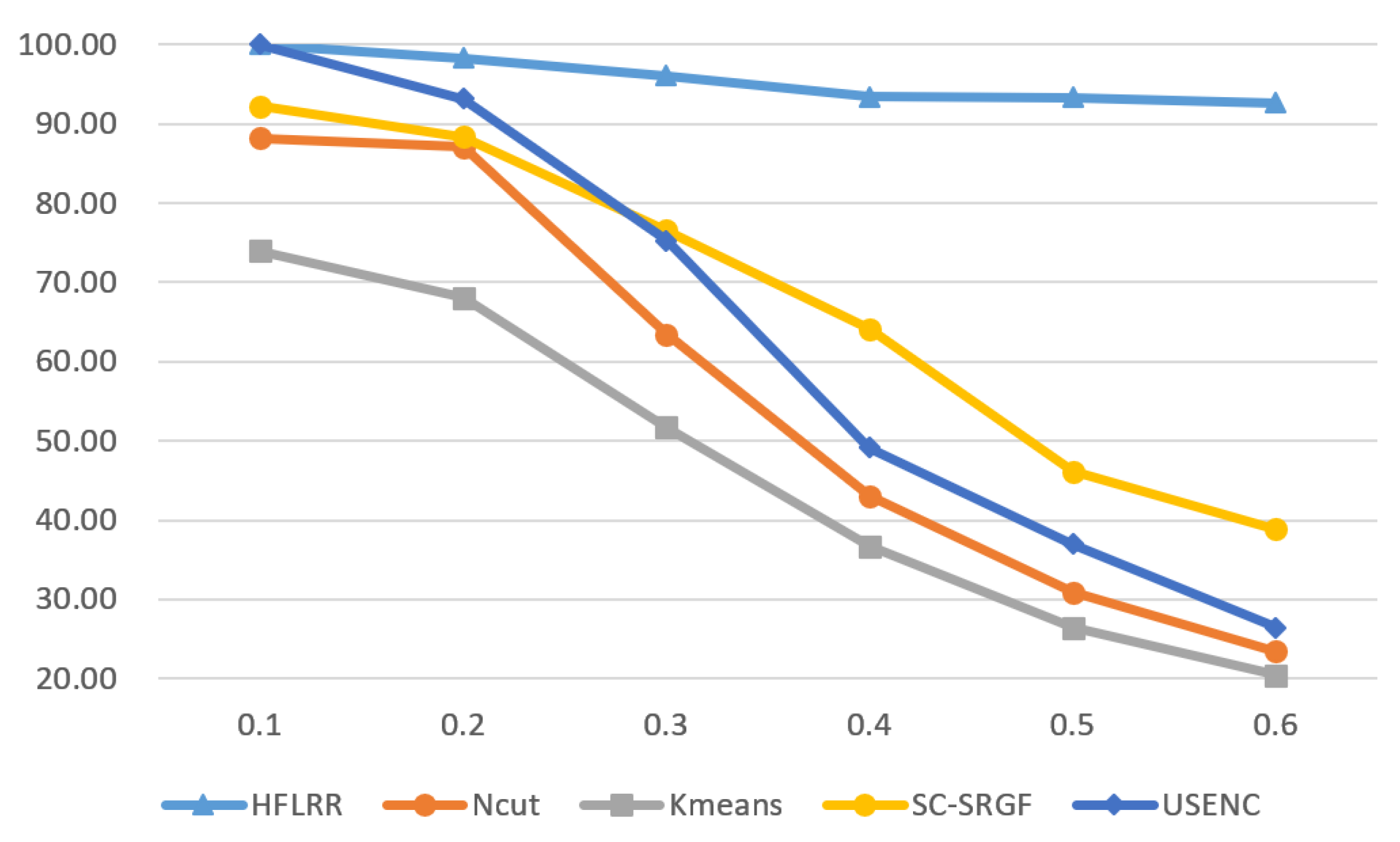
Table 1 lists the set-ups for the objective datasets and the indexes of those set-ups. Table 2 presents the clustering results with the five performance indicators mentioned above. The results in the table clearly show that HFLRSC not only achieved the best results in all datasets but also achieved 100% excellent performance in five indicators in half of the datasets. With the increase in noise intensity, the performance of the general methods would fall strongly. Specifically, in the process of Gaussian noise rising from 0.1 to 0.6, the accuracy of NCUT and K-means decreased significantly by 64.87% and 53.48%, respectively. The accuracy of HFLRSC was very stable, and even the lowest could reach a 92.62% result, which shows that our method has a very obvious effect on noise suppression and can effectively extract valuable information from low-quality IC images.
In order to make this conclusion more intuitive, we drew a broken line graph as shown in Figure 3, in which the accuracy of each algorithm changes with the transformation of Gaussian noise.
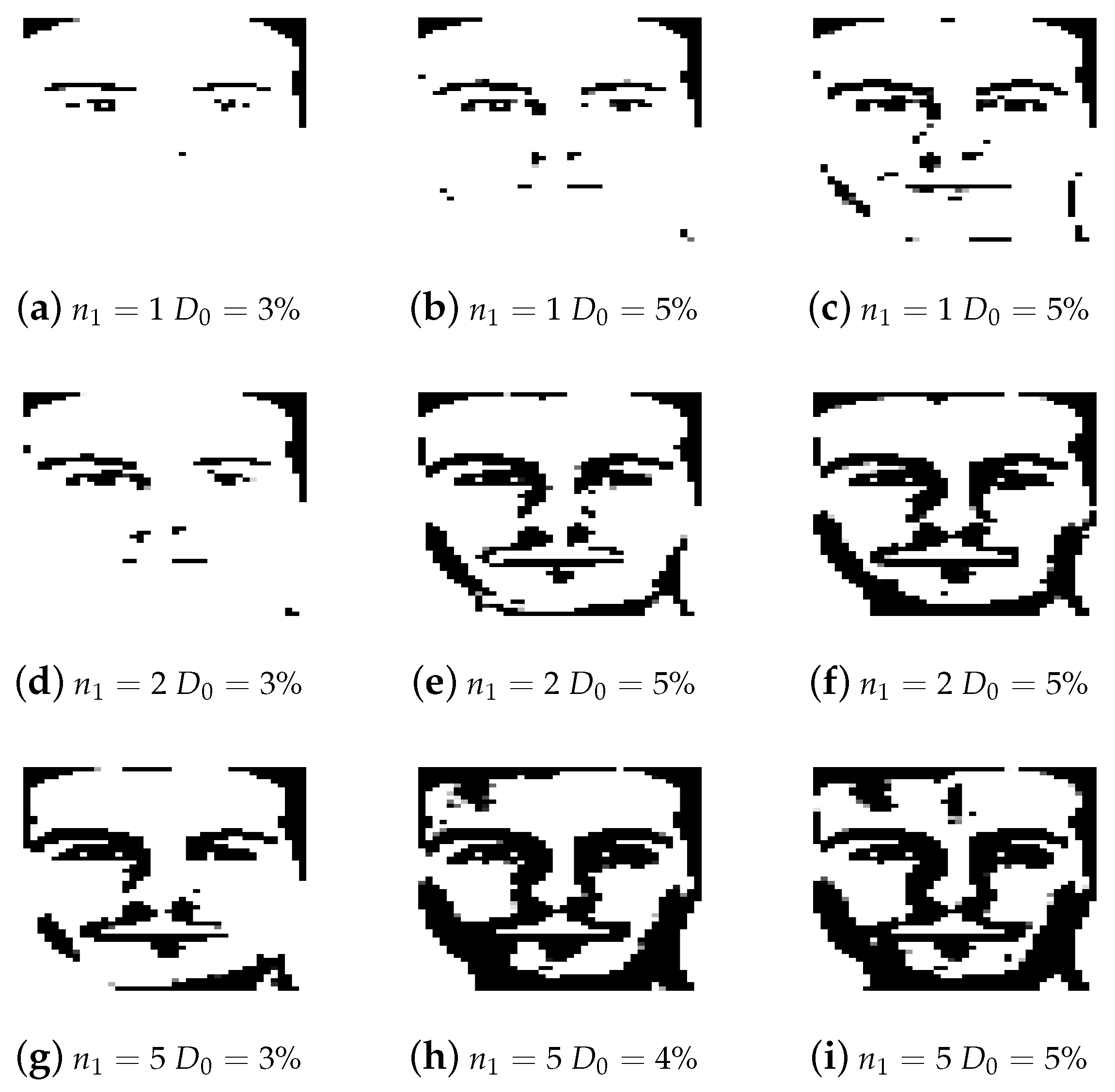
It should be noted that when extracting the HFTC, the experimental images needed to be filtered with a Butterworth filter, which has two hyperparameters: filter order and cut-off frequency. Therefore, we designed a group of face images through a Butterworth filter to intuitively express the impact of these two production parameters on the images in Figure 4. Although we fully grasped the physical meanings of these two hyperparameters, different datasets often need different combinations of two parameters, which still need the guidance of human prior knowledge. Therefore, it would lead to great progress to propose a filter to automatically find parameters.
Aside from that, the trade-off parameters of HFLRSC play roles in balancing the low rank part of the model. Because of the efficiency of HFLRSC, the values of these parameters are often set within a large range, and the best parameter value with the best result is selected by cycling all the parameter values.

5. Conclusions

In this work, we discuss how to effectively process a low-quality image of an integrated circuit. At this stage, many hardware Trojans and defect detection methods have been invented. However, most of these methods require high-quality data images. Limited by cost, high-quality images are often difficult to obtain. In addition, due to mechanical errors or processes, interference is inevitable, which may cause data corruption. Therefore, this study proposes an innovative framework called HFLRSC that attempts to develop fusion subspace clustering using low-rank constraints and high-frequency texture components for processing low-quality images in order to offer a data foundation for the subsequent verification tasks. The first step of this algorithm is using a two-dimensional Fourier transform and Butterworth filter to extract high-frequency texture components, which would be fused into the subspace clustering. The presented method achieved high clustering precision and a stable property to the level of data corruption, according to experimental results for the simulated datasets.

Author Contributions

Conceptualization, G.T. and Z.L.; Methodology, G.T.; Software, G.T.; Validation, G.T.; Formal analysis, Z.L.; Investigation, G.T.; Data curation, G.T.; Writing—original draft, G.T.; Writing—review & editing, Y.L. and J.L.; Visualization, G.T.; Supervision, Z.L., Y.C., Q.L., B.P. and J.L.; Project administration, Y.L. and J.L.; Funding acquisition, Y.C., Q.L. and Y.L. All authors have read and agreed to the published version of the manuscript.

Funding

This work was supported by the Key-Area Research & Development Program of Guangdong Province under Grants 2020B010173001 and 2020B010170002, the Open Foundation of the Guangdong Provincial Key Laboratory of Electronic Information Products Reliability Technology, and the Neuroeconomics Laboratory of Guangzhou Huashang College (2021WSYS002).

Institutional Review Board Statement

This study does not require ethical approval, and the authors chose to exclude this statement.

Informed Consent Statement

This study does not involve humans, and the authors choose to exclude this statement.

Data Availability Statement

Not applicable.

Conflicts of Interest

The authors declare no conflict of interest.

References

  1. Hao, Q.; Zhang, Z.; Xu, D.; Wang, J.; Liu, J.; Zhang, J.; Ma, J.; Wang, X. A hardware security-monitoring architecture based on data integrity and control flow integrity for embedded systems. Appl. Sci. 2022, 12, 7750. [Google Scholar] [CrossRef]
  2. Lu, H.; Capecci, D.E.; Ghosh, P.; Forte, D.; Woodard, D.L. Computer vision for hardware security. In Emerging Topics in Hardware Security; Springer: Cham, Switzerland, 2021; pp. 493–525. [Google Scholar]
  3. Wang, X.; Zhang, Z.; Xu, Y.; Zhang, L.; Yan, R.; Chen, X. Real-time minor defect recognition of pseudo-terahertz images via the improved yolo network. In Proceedings of the 2021 International Conference on Sensing, Measurement & Data Analytics in the era of Artificial Intelligence (ICSMD), Nanjing, China, 21–23 October 2021; pp. 1–6. [Google Scholar]
  4. Zhou, B.; Aksoylar, A.; Vigil, K.; Adato, R.; Tan, J.; Goldberg, B.; Ünlü, M.S.; Joshi, A. Hardware trojan detection using backside optical imaging. IEEE Trans. Comput.-Aided Des. Integr. Circuits Syst. 2020, 40, 24–37. [Google Scholar] [CrossRef]
  5. Rosso, D. Annual Semiconductor Sales Increase 21.6 Percent, Top 400 Billion for First Time; Semiconductor Industry Association: Washington, DC, USA, 2018; Volume 1. [Google Scholar]
  6. Xue, M.; Bian, R.; Wang, J.; Liu, W. Building an accurate hardware trojan detection technique from inaccurate simulation models and unlabelled ics. IET Comput. Digit. Tech. 2019, 13, 348–359. [Google Scholar] [CrossRef]
  7. Ye, M.; Zhang, D.; Yap, Y.K. Recent advances in electronic and optoelectronic devices based on two-dimensional transition metal dichalcogenides. Electronics 2017, 6, 43. [Google Scholar] [CrossRef] [Green Version]
  8. Kaintura, A.; Dhaene, T.; Spina, D. Review of polynomial chaos-based methods for uncertainty quantification in modern integrated circuits. Electronics 2018, 7, 30. [Google Scholar] [CrossRef] [Green Version]
  9. Jin, Y.; Makris, Y. Hardware trojan detection using path delay fingerprint. In Proceedings of the 2008 IEEE International Workshop on Hardware-Oriented Security and Trust, Anaheim, CA, USA, 9 June 2008; pp. 51–57. [Google Scholar]
  10. Gayatri, R.; Gayatri, Y.; Mitra, C.; Mekala, S.; Priyatharishini, M. System level hardware trojan detection using side-channel power analysis and machine learning. In Proceedings of the 2020 5th International Conference on Communication and Electronics Systems (ICCES), Coimbatore, India, 10–12 June 2020; pp. 650–654. [Google Scholar]
  11. Liakos, K.G.; Georgakilas, G.K.; Plessas, F.C. Hardware trojan classification at gate-level netlists based on area and power machine learning analysis. In Proceedings of the 2021 IEEE Computer Society Annual Symposium on VLSI (ISVLSI), Tampa, FL, USA, 7–9 July 2021; pp. 412–417. [Google Scholar]
  12. Nasr, A.A.; Abdulmageed, M.Z. Automatic feature selection of hardware layout: A step toward robust hardware trojan detection. J. Electron. Test. 2016, 32, 357–367. [Google Scholar] [CrossRef]
  13. Kulkarni, A.; Pino, Y.; Mohsenin, T. Svm-based real-time hardware trojan detection for many-core platform. In Proceedings of the 2016 17th International Symposium on Quality Electronic Design (ISQED), Santa Clara, CA, USA, 15–16 March 2016; pp. 362–367. [Google Scholar]
  14. Hasegawa, K.; Oya, M.; Yanagisawa, M.; Togawa, N. Hardware trojans classification for gate-level netlists based on machine learning. In Proceedings of the 2016 IEEE 22nd International Symposium on On-Line Testing and Robust System Design (IOLTS), Sant Feliu de Guixols, Spain, 4–6 July 2016; pp. 203–206. [Google Scholar]
  15. Kulkarni, A.; Pino, Y.; Mohsenin, T. Adaptive real-time trojan detection framework through machine learning. In Proceedings of the 2016 IEEE International Symposium on Hardware Oriented Security and Trust (HOST), McLean, VA, USA, 3–5 May 2016; pp. 120–123. [Google Scholar]
  16. Vishnupriya, R.; Devi, M.N. Hardware trojan detection using deep learning-deep stacked auto encoder. In Proceedings of the International Conference on Recent Trends in Machine Learning, IoT, Smart Cities and Applications, Hyderabad, India, 28–29 March 2021; Springer: Singapore, 2021; pp. 345–353. [Google Scholar]
  17. Yasaei, R.; Yu, S.-Y.; Faruque, M.A.A. Gnn4tj: Graph neural networks for hardware trojan detection at register transfer level. In Proceedings of the 2021 Design, Automation & Test in Europe Conference & Exhibition (DATE), Grenoble, France, 1–5 February 2021; pp. 1504–1509. [Google Scholar]
  18. Muralidhar, N.; Zubair, A.; Weidler, N.; Gerdes, R.; Ramakrishnan, N. Contrastive graph convolutional networks for hardware trojan detection in third party ip cores. In Proceedings of the 2021 IEEE International Symposium on Hardware Oriented Security and Trust (HOST), Tysons Corner, VA, USA, 12–15 December 2021. [Google Scholar]
  19. Sharma, R.; Sharma, G.; Pattanaik, M. A few shot learning based approach for hardware trojan detection using deep siamese cnn. In Proceedings of the 2021 34th International Conference on VLSI Design and 2021 20th International Conference on Embedded Systems (VLSID), Guwahati, India, 20–24 February 2021; pp. 163–168. [Google Scholar]
  20. Hasegawa, K.; Yamashita, K.; Hidano, S.; Fukushima, K.; Hashimoto, K.; Togawa, N. Node-wise hardware trojan detection based on graph learning. arXiv 2021, arXiv:2112.02213. [Google Scholar]
  21. Wei, L.; Wang, X.; Wu, A.; Zhou, R.; Zhu, C. Robust subspace segmentation by self-representation constrained low-rank representation. Neural Process. Lett. 2018, 48, 1671–1691. [Google Scholar] [CrossRef]
  22. Göçeri, E. Impact of deep learning and smartphone technologies in dermatology: Automated diagnosis. In Proceedings of the 2020 Tenth International Conference on Image Processing Theory, Tools and Applications (IPTA), Paris, France, 9–12 November 2020; pp. 1–6. [Google Scholar]
  23. Liu, G.; Lin, Z.; Yan, S.; Sun, J.; Yu, Y.; Ma, Y. Robust recovery of subspace structures by low-rank representation. IEEE Trans. Pattern Anal. Mach. Intell. 2012, 35, 171–184. [Google Scholar] [CrossRef] [PubMed] [Green Version]
  24. Bertsekas, D.P. On penalty and multiplier methods for constrained minimization. SIAM J. Control. Optim. 1976, 14, 216–235. [Google Scholar] [CrossRef]
  25. Elhamifar, E.; Vidal, R. Sparse subspace clustering: Algorithm, theory, and applications. IEEE Trans. Pattern Anal. Mach. Intell. 2013, 35, 2765–2781. [Google Scholar] [CrossRef] [PubMed]
  26. Cai, X.; Huang, D.; Wang, C.-D.; Kwoh, C.-K. Spectral clustering by subspace randomization and graph fusion for high-dimensional data. In Pacific-Asia Conference on Knowledge Discovery and Data Mining; Springer: Cham, Switzerland, 2020; pp. 330–342. [Google Scholar]
  27. Huang, D.; Wang, C.-D.; Wu, J.-S.; Lai, J.-H.; Kwoh, C.-K. Ultra-scalable spectral clustering and ensemble clustering. IEEE Trans. Knowl. Data Eng. 2019, 32, 1212–1226. [Google Scholar] [CrossRef]
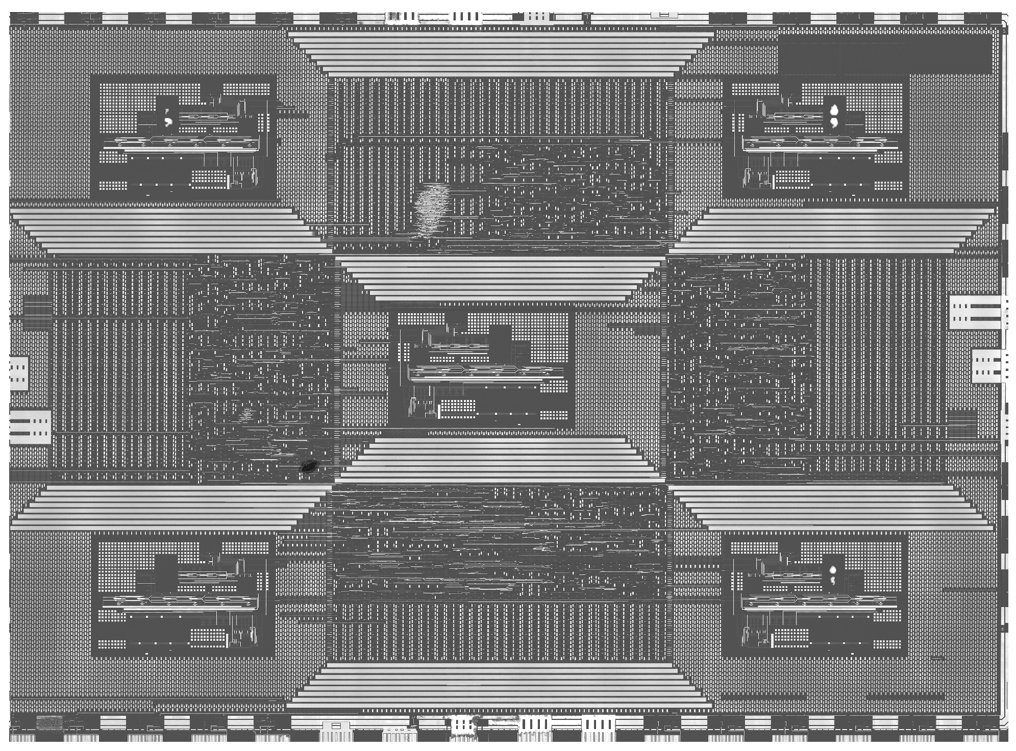
Figure 1. A scanning electron microscope image of the chip with a resolution of 6960 × 5084.
Applsci 13 00155 g001
Figure 2. Data samples corrupted by Gaussian noise with two different types of intensities and simulated defects. (a) sample a; (b) sample b.
Applsci 13 00155 g002
Figure 3. The clustering accuracy varies with the level of Gaussian noise.
Applsci 13 00155 g003
Figure 4. Figures from (ai) present the change caused by the filter’s parameters, where n 1 is the order of the filter and D 0 denotes the cut-off frequency by the percentage of the image width. As can be seen, the features of the high-frequency texture components were related to the cut-off frequency, while the thickness of the texture depended on the order of the filter.
Applsci 13 00155 g004
Table 1. Simulated datasets with different settings.
IndexNoiseDefects
1Gaussian 0.110
2Gaussian 0.210
3Gaussian 0.410
4Gaussian 0.610
5Salt-and-Pepper 0.110
6Salt-and-Pepper 0.210
7Salt-and-Pepper 0.410
8Salt-and-Pepper 0.610
9Multiplicative 0.0110
10Multiplicative 0.110
11Multiplicative 0.1510
12Multiplicative 0.210
Table 2. The clustering performances of the proposed approach and the comparison methods for the simulated datasets (1–6). The bold denotes the best results.
DatasetsMethodsACCNMIPurityFARI
1HFLRSC100.00100.00100.00100.00100.00
NCut88.2094.3190.1788.1187.01
K-means73.9485.2476.5473.4670.79
LRR97.9799.1698.5098.1197.95
SSC100.00100.00100.00100.00100.00
SC-SRGF92.2296.5894.0292.5491.89
USENC100.00100.00100.00100.00100.00
2HFLRSC98.3397.7598.3396.4996.20
NCut87.0393.3289.5086.6985.49
K-means68.0379.2370.6364.8561.20
LRR97.4298.9898.1797.6597.45
SSC93.3392.3393.3386.4785.34
SC-SRGF88.3395.3591.6789.2788.33
USENC93.1395.9593.8892.3391.64
3HFLRSC93.4091.3793.4086.4785.36
NCut43.0547.8744.7728.5922.31
K-means36.7541.2338.7826.4218.13
LRR80.8179.4681.1366.3763.50
SSC73.5067.5073.9248.1843.20
SC-SRGF64.1563.6565.9746.6142.06
USENC49.1753.7550.5835.5929.90
4HFLRSC92.6290.7292.6283.7482.37
NCut23.4225.7724.6012.172.75
K-means20.4619.5321.4511.620.00
LRR37.1238.9338.8519.5012.31
SSC27.1732.2028.8313.445.53
SC-SRGF38.9039.8240.8322.0515.26
USENC26.4628.8627.5814.475.43
5HFLRSC100.00100.00100.00100.00100.00
NCut90.9295.9192.6791.3790.59
K-means71.1082.7773.6969.3466.18
LRR100.00100.00100.00100.00100.00
SSC100.00100.00100.00100.00100.00
SC-SRGF100.00100.00100.00100.00100.00
USENC100.00100.00100.00100.00100.00
6HFLRSC100.00100.00100.00100.00100.00
NCut88.6594.1390.4588.4087.35
K-means68.0678.7570.5564.6861.15
LRR95.6798.2396.8396.0195.66
SSC100.00100.00100.00100.00100.00
SC-SRGF94.7294.9295.0291.7791.08
USENC96.6398.2297.0496.4096.08
7HFLRSC100.00100.00100.00100.00100.00
NCut78.9886.8781.4076.1674.02
K-means59.7764.9462.6749.1744.34
LRR92.0895.8393.7091.5790.83
SSC96.5896.4196.5893.4092.86
SC-SRGF90.4292.9491.5587.1486.05
USENC90.2993.7991.2588.4887.48
8HFLRSC95.2393.7595.2389.6188.75
NCut59.3066.4761.1749.1044.68
K-means48.6950.9051.6832.8926.73
LRR85.7886.9485.8376.8074.85
SSC75.5073.2875.5052.7048.12
SC-SRGF71.4771.7772.4055.8952.17
USENC54.6757.1656.4637.8132.37
9HFLRSC100.00100.00100.00100.00100.00
NCut91.3795.9792.8391.6390.87
K-means71.6784.1874.6271.7068.83
LRR99.1299.6399.3399.1799.09
SSC100.00100.00100.00100.00100.00
SC-SRGF100.00100.00100.00100.00100.00
USENC98.4698.9498.6798.0297.84
10HFLRSC100.00100.00100.00100.00100.00
NCut82.8289.0385.1080.1578.36
K-means57.2063.5161.3844.6138.83
LRR98.9099.5499.1798.9598.86
SSC95.8395.3195.8391.6991.00
SC-SRGF89.9389.7289.9583.1081.70
USENC88.7989.4689.6382.5080.99
11HFLRSC100.00100.00100.00100.00100.00
NCut71.4576.9272.7763.5560.35
K-means52.2055.6555.8936.8630.48
LRR89.3789.4190.3880.0278.26
SSC87.8385.7187.8376.0573.98
SC-SRGF83.5084.4984.7375.8573.83
USENC81.4681.7682.7970.2267.62
12HFLRSC99.1798.8899.1798.2498.10
NCut58.3263.0560.1045.0440.29
K-means46.5648.4750.2429.3922.36
LRR83.6883.7183.9269.7567.04
SSC85.5882.3785.5870.2367.62
SC-SRGF75.7373.5075.9859.8856.50
USENC46.9648.1248.5427.8621.27
Disclaimer/Publisher’s Note: The statements, opinions and data contained in all publications are solely those of the individual author(s) and contributor(s) and not of MDPI and/or the editor(s). MDPI and/or the editor(s) disclaim responsibility for any injury to people or property resulting from any ideas, methods, instructions or products referred to in the content.