
Classification and Fast Few-Shot Learning of Steel Surface Defects with Randomized Network


Abstract
:1. Introduction
- The real-time problem: The detection time should be fast enough to support the undergoing (production) process without significant loss in accuracy;
- Small target problem: Often the absolute or the relative (to the image) size of the defect is small. In our article we do not have to face this problem directly since we use benchmark datasets, however, in a real-life application, the size can have an indirect effect on the real-time problem;
- The small sample problem: The number of defect images, used either in manual parameter tuning or in automatic learning mechanisms, is often very limited;
- Unbalanced sample problem: This problem mainly exists in the task of supervised learning and relates to the previous one. Often the number of normal samples forms the majority, while the amount of defected samples only accounts for a small part. The few-shot learning problem means that we have a very unbalanced set;
- Domain shift [7]: When the dataset used in training and the dataset in practice are captured under different conditions, it can result in poor detection performance.
- Catastrophic forgetting: It was already investigated in the early 1990s [21] that a neural network is going to have a lower performance of previously trained classes when re-trained or tuned with new ones in focus. The problem is most serious if we have no training data for the already trained classes, or the dataset for re-training is unbalanced due to the missing samples from old classes. There are several approaches to avoid this case by methods such as scaling the weights of trained classifiers [22], using dual memories for storing old images and their statistics [23], or progressive incremental learning [24] where sub-networks are added incrementally to previous ones as the task is growing with new classes;
- Low number of representatives of new classes: In practical applications there is a data collection period when lots of samples are collected about the possible artifacts and used for model building. In contrast, when the system is in use for long periods, the undergoing background manufacturing processes (changes in the environment, or other influences) can result in new defect classes, which might appear in very few samples initially. In general, solutions are categorized into three main sets: using prior knowledge to augment the supervised experience (in our case data augmentation of the available few shots); modifying the model, which uses prior knowledge of known classes; and algorithmic solutions to alter the search for the best hypothesis in the given hypothesis space [25]. In extreme cases, we talk about zero-shot learning: when a new type of defect appears, it is a question whether we are able to classify it as a new class or if it will fall into an existing category. We would like to avoid this latter case and thus we have to create a new category and be able to tune the existing model to consider it [10,26,27];
- Complexity of updating the classifiers: It is a practical problem during the application of deep learning models that the re-training or fine-tuning of new or updated models can be time consuming or computationally very complex. A fast adaptation to the extended set of classes and easy training procedures are needed for real-life applications.
- Instead of re-tailoring old models or defining new deep neural architectures, we show that a well-proven and efficient deep neural network (DNN) (EfficientNet-B7 [28]) can give the best known accuracy for the classification of steel surface defects on two major benchmark datasets;
- We propose a novel architecture designed for incremental learning with the following features: it avoids the catastrophic forgetting of old classes, it has good performance in case of very few shots, and it can be trained very fast for new classes. To achieve this, we apply randomized networks concatenated to the feature extraction of a pre-trained DNN. The computation of its weights can be done very efficiently by the Moore–Penrose generalized inverse.
2. Related Works
2.1. Detection and Classification of Steel Surface Defects
2.2. Zero-Shot Learning
2.3. Few-Shot Learning
3. Proposed Methods
3.1. Classification of Defects with EfficientNet-B7
3.2. Few-Shot Learning of Defects
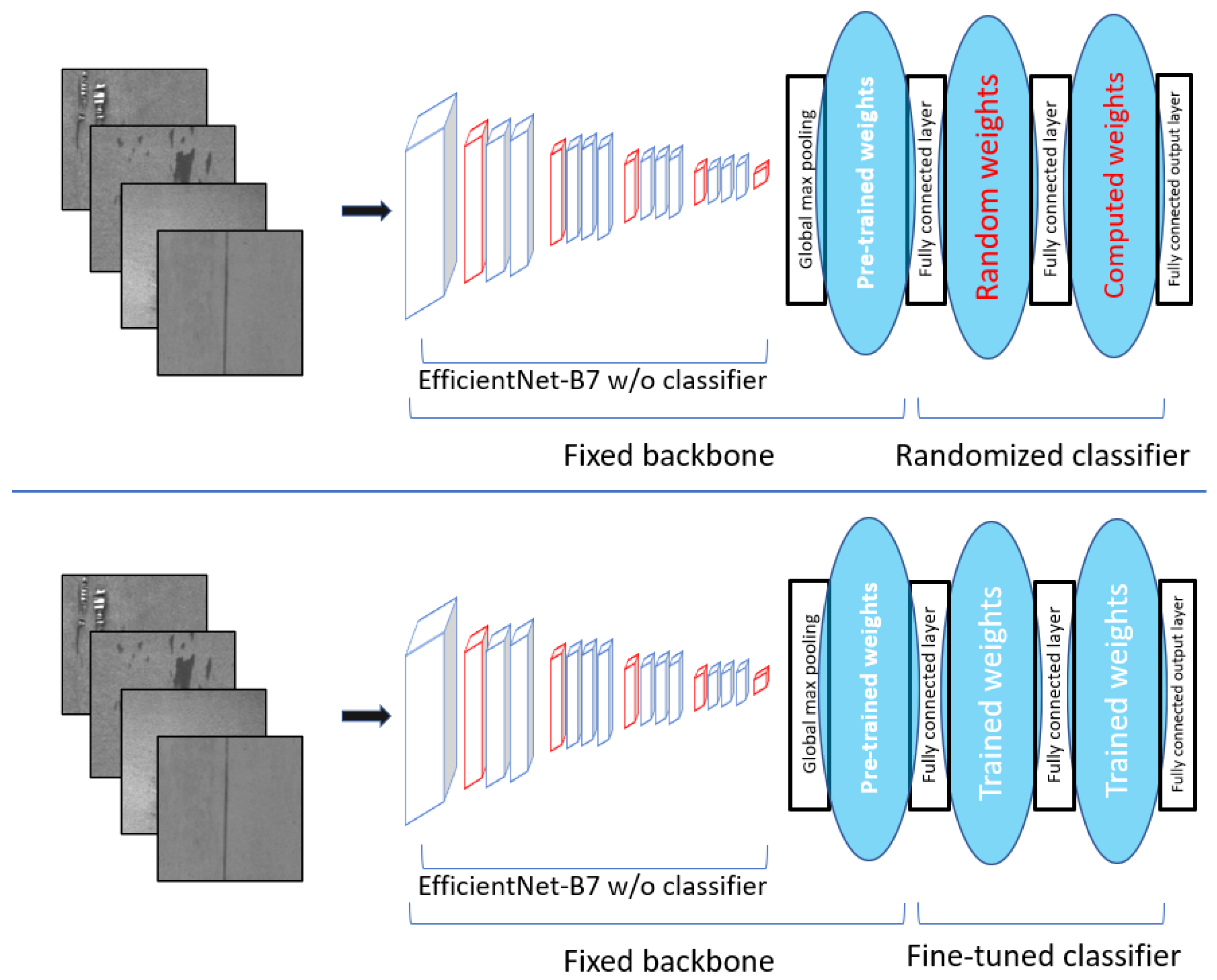
- The backbone is a deep neural network with an output feature vector of relatively large dimension (1024). We have chosen EfficientNet-B7 for this task due to its design for optimal size, structure, and accuracy. The task of the backbone is to adapt from ImageNet weights to steel surface defects with high accuracy with conventional training;
- The back-end structure, for the further processing of extracted features, is a two-layer neural network where the first layer contains random weights. Since the backbone is previously fine-tuned to a set of known classes of steel surface defects, the task of this back end is to quickly learn the new classes based on the features of the backbone.
- EfficientNet-B7 is very efficient for the classification of steel surface defects (see Section 5). Near its output, it still has a lengthy (hopefully rich) feature vector used by our back end;
- The back end has a random layer responsible for the generalization of fine-tuned feature values suitable for learning unseen classes;
- Since the back end has only one layer to be trained, it can be explicitly computed with algebraic computations without a lengthy backpropagation method. These computations give optimal solutions in the least-squares sense.
3.2.1. Randomized Weights for Generalization and Fast Tuning
3.2.2. Randomizing EfficientNet Features
| Algorithm 1: Incremental training with few shots with randomized EfficientNet features. |
 |
4. The Benchmark Datasets
4.1. Northeastern University Surface Defect Database
4.2. Xsteel Surface Defect Dataset (X-SSD)
- Red iron sheet: high silicon content in steel and high heating temperature of slab;
- Iron sheet ash: accumulated contamination (e.g., dust, oil) falls onto the surface;
- Inclusions: inclusion of slags in the steel;
- Surface scratches: hot-rolling area with projections—dead or passive rolls can cause friction on the surface;
- Finishing-roll printing: the slippage between the work roll and the support roll can result in dot and short-strip damages on the surface of the work roll;
- Oxide scale-of-plate system: if the roller table is damaged it can also damage the surface of the rolled piece where the iron oxide particles can accumulate and they can be rolled into the steel in the subsequent rolling process;
- Oxide scale-of-temperature system: it can be caused by many things, such as improper temperature settings, high carbon content, and unwanted intense oxidation.
5. Experimental Results of Classification and Its Discussion
- Random rotations between and ;
- Vertical flipping;
- Horizontal flipping;
- Zooming randomly between 0 and 20% in size.
5.1. Classification Results on the NEU Dataset
5.2. Classification Results on the X-SSD Dataset
6. Testing Few-Shot Learning with EffNet+RC
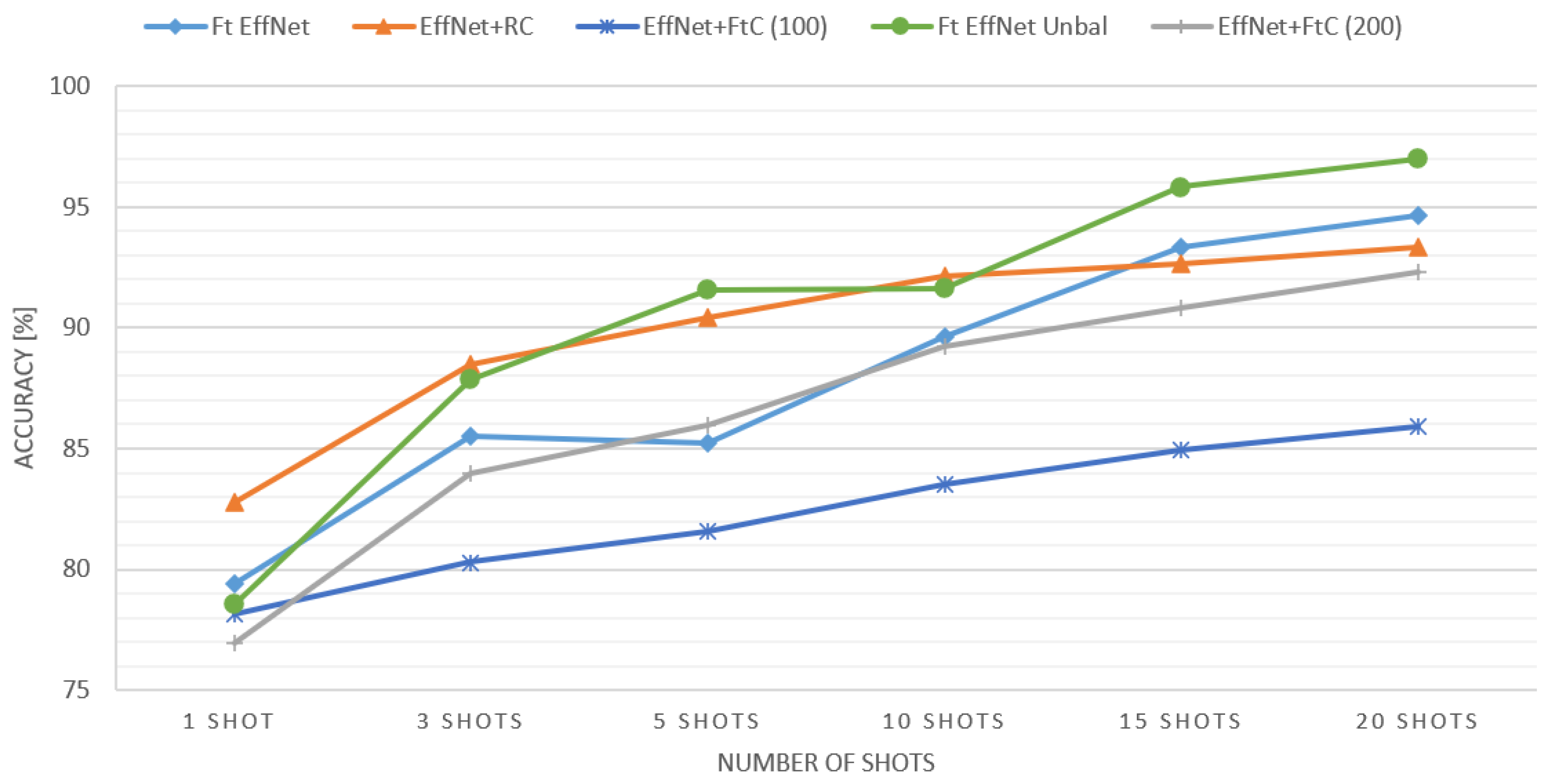
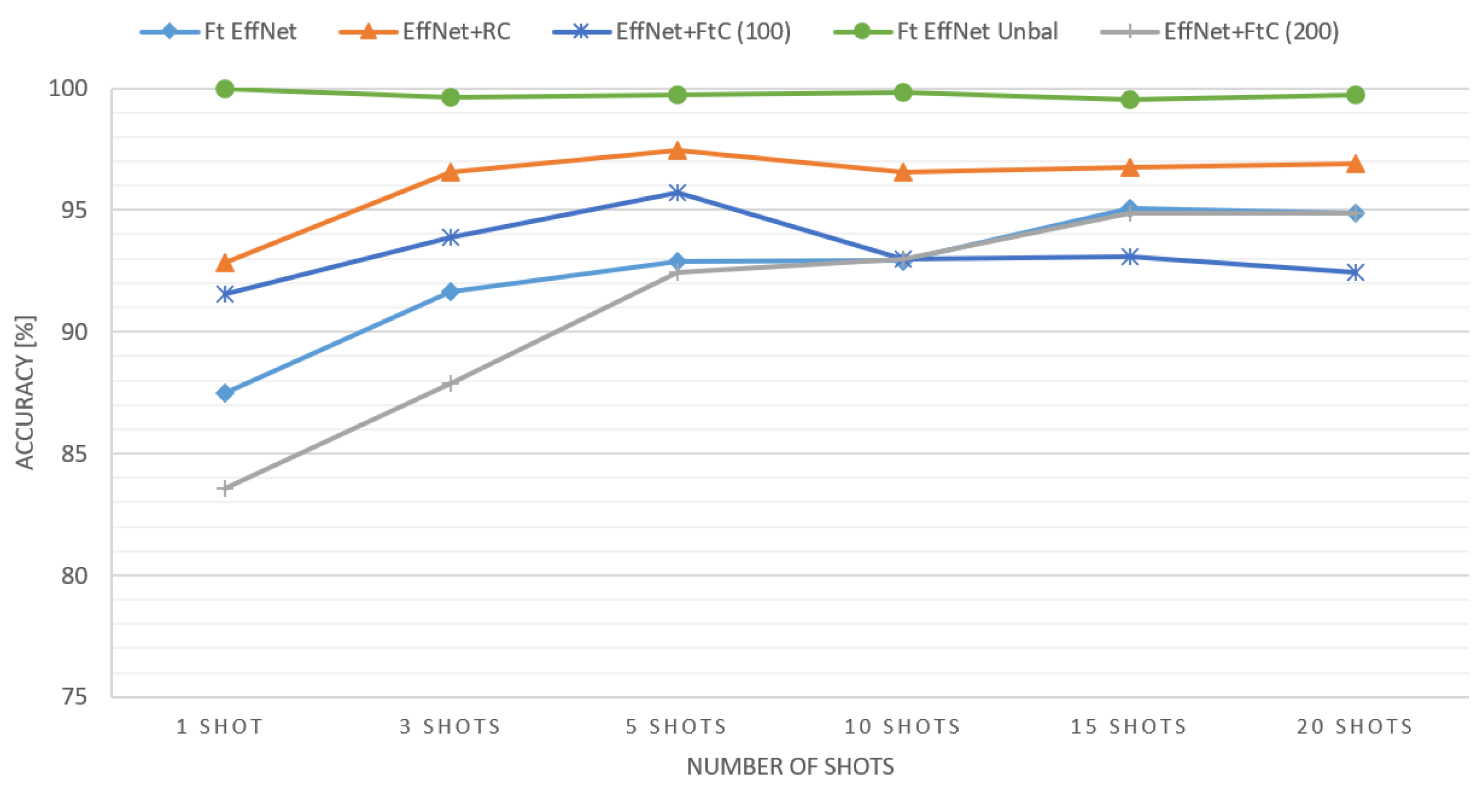
- EffNet+FtC: This network only differs from EffNet+RC in that instead of random weights, backpropagation fine-tuned weights are used in the classifier, and the backbone is still frozen see Figure 5. The purpose of this network is to learn the effect of randomization (when compared to EffNet+RC). We ran the training for 100 and 200 epochs;
- Ft EffNet: Fine-tuned EfficienNet-B7 by few shots (being augmented). To keep the fine-tuning dataset balanced the ratio of base classes is the same as of the new ones;
- Ft EffNet Unbal: Fine-tuned EfficientNet-B7 with unbalanced data. The same as above, but possibly all samples from the base classes were used in fine-tuning. This means unbalanced training, since new classes were sampled only by the few shots.
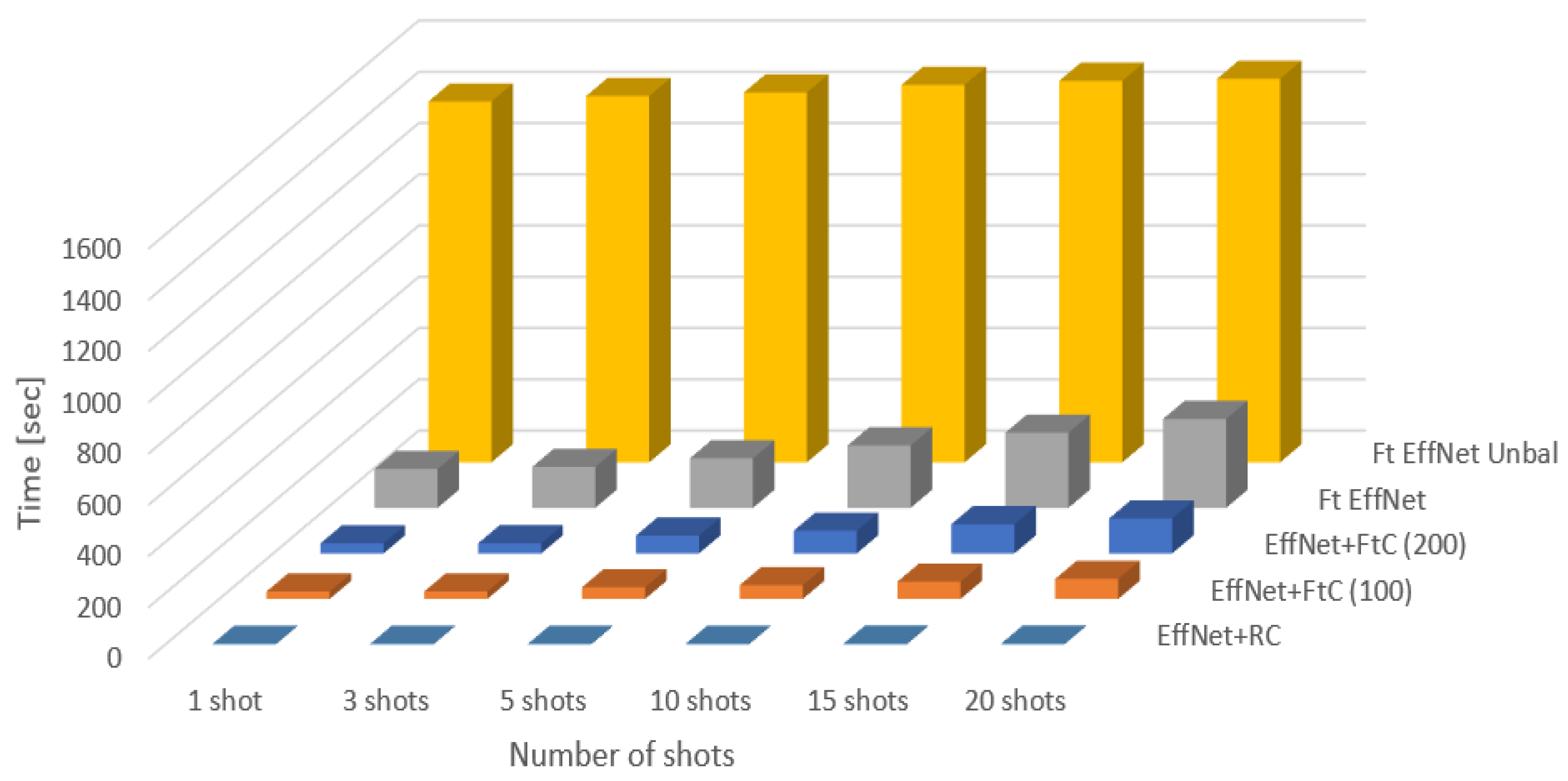
Time Complexity
7. Summary and Future Work
- We showed that state-of-the-art DNNs (namely EfficientNet-B7) can solve the classification of steel surface defects of the two often-used datasets almost perfectly, and that they were superior to other made-to-measure techniques;
- We applied randomized networks, concatenated to the feature extraction of a pre-trained DNN, to give a solution for the few-shot problem. Since the computation of its weights can be done very efficiently by the Moore–Penrose generalized inverse, the solution has the following advantages:
- Regarding very few shots (one to three), our model outperformed other variants when classifying both old and newly appearing classes of steel surface defects;
- Regarding the base classes, catastrophic forgetting could be avoided;
- The fine-tuning for new classes or shots is significantly faster than the fine-tuning of any conventional DNNs.
Author Contributions
Funding
Institutional Review Board Statement
Informed Consent Statement
Data Availability Statement
Acknowledgments
Conflicts of Interest
Abbreviations
| RC | Randomized Classifier |
| X-SSD | Xsteel Surface Defect dataset |
| NEU | Northeastern University Surface Defect Database |
| DNN | Deep Neural Network |
| CNN | Convolutional Neural Network |
| YOLOv4 | You Look Only Once Network Version 4 |
| FPN | Feature Pyramid Network |
| R-CNN | Region-Based Convolutional Neural Network |
| RestNet | Residual Neural Network |
| MAP | Mean Average Precision |
| CPN | Classification Priority Network |
| MG-CNN | Multiple Group Convolutional Neural Network |
| DDN | Defect Detection Network |
| MFN | Multi-level Feature Fusion Network |
| ROI | Region of Interest |
| DA | Domain Adaptation |
| ACNN | Adaptive Learning Rate of the Convolutional Neural Networks |
| VGG19 | Visual Geometry Group from Oxford 19 |
| DeVGG19 | Decode VGG19 |
| SSIM | Structural Similarity Index Measure |
| GCN | Graph Convolution Networks |
| MMGCN | Multiple Micrographs Graph Convolutional Network |
| k-NN | k-Nearest Neighbor Graph |
| SENet | Squeeze-and-Excitation Networks |
| RN | Relation Network |
| CD-FSL | Cross-Domain Few-Shot Learning |
| BSR | Batch Spectrum Regularization |
| MNIST | Modified National Institute of Standards and Technology Database |
| CIFAR | Canadian Institute for Advanced Research |
| SLFN | Single Layer Feed-Forward Neural Network |
| RVFL | Random Vector Functional Links Network |
| ELM | Extreme Learning Machines |
| EffNet+RC | EfficientNet-B7 Backbone and the Randomized Classifier (RC) |
| VGG16 | Visual Geometry Group from Oxford |
| ExtVGG16 | Extended VGG16 |
| EffNet | EfficientNet |
| EffNet+FtC | Frozen EfficientNet Backbone with Backpropagation Fine-Tuned Weights |
| Ft EffNet | Fine-tuned EfficienNet-B7 |
| Ft EffNet Unbal | Fine-tuned EfficientNet-B7 with Unbalanced Data |
Appendix A

| Task | Title | Description | Dataset | Accuracy | MAP |
|---|---|---|---|---|---|
| Detection and classification methods | |||||
| Detection of metal surface defects based on YOLOv4 algorithm [5]. | Improvement of YOLOv4 architecture by adding a feature pyramid network (FPN) module after sampling, on the so-called neck part of the network. | NEU | 92.5% | - | |
| A new steel defect detection algorithm based on deep learning [4]. | Improved Faster R-CNN model by using deformable convolutions and multi-level feature fusion. | NEU-DET | - | 75.2 | |
| Defect detection of hot-rolled steels with a new object detection framework called classification priority network [6]. | Classification priority network: two-stage classification. | Author dataset | 96.00% | - | |
| An end-to-end steel surface defect detection approach via fusing multiple hierarchical features [3]. | The processing goes through the steps: 1. feature map generation by ResNet; 2. multi-level feature fusion network; 3. region proposal network; 4. classifier and a bounding box regressor. | NEU-DET | 99.67% | 82.3 | |
| Visual inspection of steel surface defects based on domain adaptation and adaptive convolutional neural network [7]. | It combines domain adaptation and the adaptive learning rate of the convolutional neural networks to handle the changes during the production. Furthermore, applies an additional domain classifier and a constraint on label probability distribution to enable cross-domain and cross-task recognition, and to account for the lack of labels in a new domain. | NEU | 99.00% | - | |
| A steel surface defect recognition algorithm based on improved deep learning network model using feature visualization and quality evaluation [8]. | A steel surface defect classification technique fine-tuned with the help of a feature visualization network was proposed. | NEU | 89.86% | - | |
| Recognition of scratches and abrasions on metal surfaces using a 534 classifier based on a convolutional neural network [9]. | Different versions of ResNet were investigated to classify three kinds of defects on metal surfaces. | NEU | 97.10% | - | |
| Classification of surface defects on steel strip images using convolution neural network and support vector machine [30]. | A modified AlexNet for feature extraction, where the classification was solved with a support vector machine. | NEU | 99.70% | - | |
| Zero-shot learning and classification of steel surface defects [10]. | VGG16 was extended with several layers for classification (ExtVGG16). | NEU | 100.00% | - | |
| Zero-shot Learning | |||||
| Zero-sample surface defect detection and classification based on semantic feedback neural network [27]. | Word vectors, extracted from an auxiliary knowledge source, are used to solve the zero-shot learning problem. | Cylinder-liner defect dataset (CLSDD) | 89.28% | - | |
| One-shot recognition of manufacturing defects in steel surfaces [26]. | A Siamese neural network is used to decide whether two input samples belong to the same class or not. | NEU | 83.22% | - | |
| Zero-shot learning and classification of steel surface defects [10]. | Similar to ref. [26] but with a more efficient structure. | NEU | 85.8% | - | |
| Few-shot Learning | |||||
| Steel Surface defect classification based on small sample learning [32]. | Comparing ResNet, DenseNet, and MobileNet for feature extraction and mean subtraction and L2 normalization for feature transformation. For one-shot learning a nearest neighbor approach, whereas for the multi-shot setting the average value of known sample feature vectors are used. | NEU | 92.33% | - | |
| A new graph-based semi-supervised method for surface defect classification [33]. | A semi-supervised learning model called multiple micrographs graph convolutional network was proposed, which learns from both labeled and unlabeled samples. | NEU | 99.72% | - | |
| Few-shot learning approach for 3D defect detection in lithium battery [35]. | Training images were used to fine-tune a pre-trained ResNet10 model, then a k-NN graph is built to evaluate the distance between samples, including both the labeled and the unlabeled ones. To refine the scoring of samples a label propagation method was used. | Lithium batteries | 97.17% | - | |
| Fabric defect classification using prototypical network of few-shot learning algorithm [37]. | A meta-training prototype-based approach to handle the unbalanced data caused by the newly arriving error classes having only few shots. Training is cut into episodes, after each episode the model is fine-tuned. | Textile | 99.72% | - |
References
- Feng, X.; Gao, X.; Luo, L. X-SDD: A new benchmark for hot rolled steel strip surface defects setection. Symmetry 2021, 13, 706. [Google Scholar] [CrossRef]
- Song, K.; Yan, Y. A noise robust method based on completed local binary patterns for hot-rolled steel strip surface defects. Appl. Surf. Sci. 2013, 285, 858–864. [Google Scholar] [CrossRef]
- He, Y.; Song, K.; Meng, Q.; Yan, Y. An end-to-end steel surface defect detection approach via fusing multiple hierarchical features. IEEE Trans. Instrum. Meas. 2019, 69, 1493–1504. [Google Scholar] [CrossRef]
- Zhao, W.; Chen, F.; Huang, H.; Li, D.; Cheng, W. A new steel defect detection algorithm based on deep learning. Comput. Intell. Neurosci. 2021, 2021, 13. [Google Scholar] [CrossRef]
- Zhao, H.; Yang, Z.; Li, J. Detection of metal surface defects based on YOLOv4 algorithm. J. Phys. Conf. Ser. IOP Publ. 2021, 1907, 012043. [Google Scholar] [CrossRef]
- He, D.; Xu, K.; Zhou, P. Defect detection of hot rolled steels with a new object detection framework called classification priority network. Comput. Ind. Eng. 2019, 128, 290–297. [Google Scholar] [CrossRef]
- Zhang, S.; Zhang, Q.; Gu, J.; Su, L.; Li, K.; Pecht, M. Visual inspection of steel surface defects based on domain adaptation and adaptive convolutional neural network. Mech. Syst. Signal Process. 2021, 153, 107541. [Google Scholar] [CrossRef]
- Guan, S.; Lei, M.; Lu, H. A steel surface defect recognition algorithm based on improved deep learning network model using feature visualization and quality evaluation. IEEE Access 2020, 8, 49885–49895. [Google Scholar] [CrossRef]
- Konovalenko, I.; Maruschak, P.; Brevus, V.; Prentkovskis, O. Recognition of scratches and abrasions on metal surfaces using a classifier based on a convolutional neural network. Metals 2021, 11, 549. [Google Scholar] [CrossRef]
- Nagy, A.M.; Czúni, L. Zero-shot learning and classification of steel surface defects. In Proceedings of the Fourteenth International Conference on Machine Vision (ICMV 2021). International Society for Optics and Photonics, Rome, Italy, 8–14 November 2021; Volume 12084, pp. 386–394. [Google Scholar]
- Chen, Y.; Ding, Y.; Zhao, F.; Zhang, E.; Wu, Z.; Shao, L. Surface defect detection methods for industrial products: A review. Appl. Sci. 2021, 11, 7657. [Google Scholar] [CrossRef]
- Seff, A.; Beatson, A.; Suo, D.; Liu, H. Continual learning in generative adversarial nets. arXiv 2017, arXiv:1705.08395. [Google Scholar]
- Shin, H.; Lee, J.K.; Kim, J.; Kim, J. Continual learning with deep generative replay. arXiv 2017, arXiv:1705.08690. [Google Scholar]
- Parisi, G.I.; Kemker, R.; Part, J.L.; Kanan, C.; Wermter, S. Continual lifelong learning with neural networks: A review. Neural Netw. 2019, 113, 54–71. [Google Scholar] [CrossRef] [PubMed]
- Belouadah, E.; Popescu, A. DeeSIL: Deep-shallow incremental learning. In European Conference on Computer Vision; Springer: Cham, Switzerland, 2018; pp. 151–157. [Google Scholar]
- Castro, F.M.; Marín-Jiménez, M.J.; Guil, N.; Schmid, C.; Alahari, K. End-to-end incremental learning. In Proceedings of the European Conference on Computer Vision (ECCV), Munich, Germany, 8–14 September 2018; pp. 233–248. [Google Scholar]
- He, C.; Wang, R.; Shan, S.; Chen, X. Exemplar-Supported Generative Reproduction for Class Incremental Learning. In Proceedings of the 2018 British Machine Vision Conference, Newcastle, UK, 3–6 September 2018; p. 98. [Google Scholar]
- Rebuffi, S.A.; Kolesnikov, A.; Sperl, G.; Lampert, C.H. iCarL: Incremental classifier and representation learning. In Proceedings of the IEEE Conference on Computer Vision and Pattern Recognition, Honolulu, HI, USA, 21–26 July 2017; pp. 2001–2010. [Google Scholar]
- Luo, Y.; Yin, L.; Bai, W.; Mao, K. An appraisal of incremental learning methods. Entropy 2020, 22, 1190. [Google Scholar] [CrossRef] [PubMed]
- Boukli Hacene, G.; Gripon, V.; Farrugia, N.; Arzel, M.; Jezequel, M. Transfer incremental learning using data augmentation. Appl. Sci. 2018, 8, 2512. [Google Scholar] [CrossRef] [Green Version]
- Ratcliff, R. Connectionist models of recognition memory: Constraints imposed by learning and forgetting functions. Psychol. Rev. 1990, 97, 285. [Google Scholar] [CrossRef]
- Belouadah, E.; Popescu, A. Scail: Classifier weights scaling for class incremental learning. In Proceedings of the IEEE/CVF Winter Conference on Applications of Computer Vision, Snowmass, CO, USA, 1–5 March 2020; pp. 1266–1275. [Google Scholar]
- Belouadah, E.; Popescu, A. Il2m: Class incremental learning with dual memory. In Proceedings of the IEEE/CVF International Conference on Computer Vision, Seoul, Korea, 27 October–2 November 2019; pp. 583–592. [Google Scholar]
- Siddiqui, Z.A.; Park, U. Progressive convolutional neural network for incremental learning. Electronics 2021, 10, 1879. [Google Scholar] [CrossRef]
- Wang, Y.; Yao, Q.; Kwok, J.T.; Ni, L.M. Generalizing from a few examples: A survey on few-shot learning. ACM Comput. Surv. 2020, 53, 1–34. [Google Scholar] [CrossRef]
- Deshpande, A.M.; Minai, A.A.; Kumar, M. One-shot recognition of manufacturing defects in steel surfaces. Procedia Manuf. 2020, 48, 1064–1071. [Google Scholar] [CrossRef]
- Guo, Y.; Fan, Y.; Xiang, Z.; Wang, H.; Meng, W.; Xu, M. Zero-sample surface defect detection and classification based on semantic feedback neural network. arXiv 2021, arXiv:2106.07959. [Google Scholar]
- Tan, M.; Le, Q. Efficientnet: Rethinking model scaling for convolutional neural networks. In Proceedings of the International Conference on Machine Learning, Long Beach, CA, USA, 3 June 2019; pp. 6105–6114. [Google Scholar]
- Schlagenhauf, T.; Yildirim, F.; Brückner, B.; Fleischer, J. Siamese basis function networks for defect classification. arXiv 2020, arXiv:2012.01338. [Google Scholar]
- Boudiaf, A.; Benlahmidi, S.; Harrar, K.; Zaghdoudi, R. Classification of surface defects on steel strip images using convolution neural network and support vector machine. J. Fail. Anal. Prev. 2022, V22, 1–11. [Google Scholar] [CrossRef]
- Pennington, J.; Socher, R.; Manning, C.D. Glove: Global vectors for word representation. In Proceedings of the Conference on Empirical Methods in Natural Language Processing (EMNLP), Doha, Qatar, 25–29 October 2014; pp. 1532–1543. [Google Scholar]
- Wu, S.; Zhao, S.; Zhang, Q.; Chen, L.; Wu, C. Steel Surface defect classification based on small sample learning. Appl. Sci. 2021, 11, 11459. [Google Scholar] [CrossRef]
- Wang, Y.; Gao, L.; Gao, Y.; Li, X. A new graph-based semi-supervised method for surface defect classification. Robot. Comput.-Integr. Manuf. 2021, 68, 102083. [Google Scholar] [CrossRef]
- Yang, L.; Zhan, X.; Chen, D.; Yan, J.; Loy, C.C.; Lin, D. Learning to cluster faces on an affinity graph. In Proceedings of the IEEE/CVF Conference on Computer Vision and Pattern Recognition, Long Beach, CA, USA, 15–20 June 2019; pp. 2298–2306. [Google Scholar]
- Wu, K.; Tan, J.; Li, J.; Liu, C. Few-shot learning approach for 3D defect detection in lithium battery. J. Phys. Conf. Ser. IOP Publ. 2021, 1884, 012024. [Google Scholar] [CrossRef]
- Zhou, D.; Bousquet, O.; Lal, T.; Weston, J.; Schölkopf, B. Learning with local and global consistency. Adv. Neural Inform. Process. Syst. 2003, 16. [Google Scholar]
- Zhan, Z.; Zhou, J.; Xu, B. Fabric defect classification using prototypical network of few-shot learning algorithm. Comput. Ind. 2022, 138, 103628. [Google Scholar] [CrossRef]
- Russakovsky, O.; Deng, J.; Su, H.; Krause, J.; Satheesh, S.; Ma, S.; Huang, Z.; Karpathy, A.; Khosla, A.; Bernstein, M.; et al. Imagenet large scale visual recognition challenge. Int. J. Comput. Vision 2015, 115, 211–252. [Google Scholar] [CrossRef] [Green Version]
- LeCun, Y.; Bottou, L.; Bengio, Y.; Haffner, P. Gradient-based learning applied to document recognition. Proc. IEEE 1998, 86, 2278–2324. [Google Scholar] [CrossRef] [Green Version]
- Krizhevsky, A.; Hinton, G. Learning Multiple Layers of Features from Tiny Images; Department of Computer Science, University of Toronto: Toronto, ON, Canada, 2009. [Google Scholar]
- Kyriakides, G.; Margaritis, K. An introduction to neural architecture search for convolutional networks. arXiv 2020, arXiv:2005.11074. [Google Scholar]
- Sandler, M.; Howard, A.; Zhu, M.; Zhmoginov, A.; Chen, L.C. MobileNetV2: Inverted residuals and linear bottlenecks. In Proceedings of the IEEE Conference on Computer Vision and Pattern Recognition, Salt Lake City, UT, USA, 18–23 June 2018; pp. 4510–4520. [Google Scholar]
- Kiss, N.; Czùni, L. Mushroom image classification with CNNs: A case-study of different learning strategies. In Proceedings of the 12th International Symposium on Image and Signal Processing and Analysis (ISPA), Zagreb, Croatia, 13–15 September 2021; pp. 165–170. [Google Scholar]
- Hridoy, R.H.; Akter, F.; Rakshit, A. Computer vision based skin disorder recognition using EfficientNet: A transfer learning approach. In Proceedings of the 2021 International Conference on Information Technology (ICIT), Amman, Jordan, 14–15 July 2021; pp. 482–487. [Google Scholar]
- Ab Wahab, M.N.; Nazir, A.; Ren, A.T.Z.; Noor, M.H.M.; Akbar, M.F.; Mohamed, A.S.A. Efficientnet-lite and hybrid CNN-KNN implementation for facial expression recognition on raspberry pi. IEEE Access 2021, 9, 134065–134080. [Google Scholar] [CrossRef]
- Garg, H.; Sharma, B.; Shekhar, S.; Agarwal, R. Spoofing detection system for e-health digital twin using EfficientNet convolution neural network. Multimed. Tools Appl. 2022, 1–16. [Google Scholar] [CrossRef]
- Xu, R.; Lin, H.; Lu, K.; Cao, L.; Liu, Y. A forest fire detection system based on ensemble learning. Forests 2021, 12, 217. [Google Scholar] [CrossRef]
- Yousfi, Y.; Butora, J.; Fridrich, J.; Fuji Tsang, C. Improving efficientnet for JPEG steganalysis. In Proceedings of the 2021 ACM Workshop on Information Hiding and Multimedia Security, virtual event Belgium, 22–25 June 2021; pp. 149–157. [Google Scholar]
- Gao, F.; Sa, J.; Wang, Z.; Zhao, Z. Cassava disease detection method based on EfficientNet. In Proceedings of the 7th International Conference on Systems and Informatics (ICSAI), Chongqing, China, 13–15 November 2021; pp. 1–6. [Google Scholar]
- Schmidt, W.F.; Kraaijveld, M.A.; Duin, R.P. Feed forward neural networks with random weights. In Proceedings of the International Conference on Pattern Recognition, The Hague, The Netherlands, 30 August–3 September 1992; p. 1. [Google Scholar]
- Pao, Y.H.; Park, G.H.; Sobajic, D.J. Learning and generalization characteristics of the random vector functional-link net. Neurocomputing 1994, 6, 163–180. [Google Scholar] [CrossRef]
- Huang, G.B.; Zhu, Q.Y.; Siew, C.K. Extreme learning machine: Theory and applications. Neurocomputing 2006, 70, 489–501. [Google Scholar] [CrossRef]
- Suganthan, P.N.; Katuwal, R. On the origins of randomization-based feedforward neural networks. Appl. Soft Comput. 2021, 105, 107239. [Google Scholar] [CrossRef]
- Cao, W.; Wang, X.; Ming, Z.; Gao, J. A review on neural networks with random weights. Neurocomputing 2018, 275, 278–287. [Google Scholar] [CrossRef]
- Moore, E.H. On the reciprocal of the general algebraic matrix. Bull. Am. Math. Soc. 1920, 26, 394–395. [Google Scholar]
- Lv, X.; Duan, F.; Jiang, J.j.; Fu, X.; Gan, L. Deep metallic surface defect detection: The new benchmark and detection network. Sensors 2020, 20, 1562. [Google Scholar] [CrossRef] [Green Version]
- Schlagenhauf, T.; Landwehr, M.; Fleischer, J. Industrial Machine Tool Element Surface Defect Dataset; Karlsruher Institut für Technologie: Karlsruhe, Germany, 2021. [Google Scholar]


| OS | CPU | GPU | Keras | Python |
|---|---|---|---|---|
| Ubuntu 18.04 | Intel(R) Xeon(R) Gold 5115 CPU @ 2.40 GHz | NVIDIA Quadro P6000 GPU with 24 GB RAM | 2.3.0 | 3.6.9 |
| Model | MMGCN 1 [33] | SBF-Net | ResNet50+MFN | Res-Net50 | MVM-VGG | Res-Net34 | Decaf | VSD 2 [8] | ResNet43+MFN | AECLBP | OVERFEAT | ClassicResNet50 | BYEC | ExtVGG16 [10] | EfficientNet-B7 |
|---|---|---|---|---|---|---|---|---|---|---|---|---|---|---|---|
| Accuracy | 99.72% | 99.72% | 99.67% | 99.67% | 99.5% | 99.33% | 99.27% | 89.17% | 99.17% | 98.93% | 98.7% | 98.67% | 96.3% | 100% | 100% |
| Model | EspNet-v2 | GhostNet | ShuffleNet | SqueezeNet | Xception | VGG16 | ResNet50 | ResNet101 | ResNet152 | RepVGGB1g2 | RepVGGB3g4 | RepVGGB3g4+SA | ExtVGG16 | EfficientNet-B7 |
|---|---|---|---|---|---|---|---|---|---|---|---|---|---|---|
| Accuracy | 89.95% | 88.72% | 87.50% | 91.42% | 90.44% | 92.65% | 93.87% | 87.01% | 92.16% | 88.97% | 91.67% | 95.10% | 99.00% | 99.26% |
| Macro-recall | 84.19% | 87.87% | 85.84% | 83.21% | 87.39% | 90.46% | 89.41% | 88.30% | 89.41% | 82.04% | 85.28% | 93.92% | 98.00% | 98.71% |
| Macro-precision | 88.28% | 86.93% | 84.83% | 90.36% | 89.41% | 91.70% | 93.45% | 88.18% | 91.41% | 90.79% | 88.46% | 95.16% | 99.00% | 99.14% |
| Macro- score | 84.28% | 87.07% | 84.68% | 84.15% | 88.25% | 90.92% | 90.02% | 87.05% | 89.92% | 81.58% | 84.94% | 93.25% | 98.57% | 99.00% |
| Model | All Images of X-SSD: 1360 | |||
|---|---|---|---|---|
| Training: 1092 | Testing: 268 | |||
| Base Classes: 835 | New Classes: 257 | Bases Classes: 206 | New Classes: 62 | |
| EffNet backbone | All | None | None | None |
| EffNet+RC | K shots | K shots | All | All |
| EffNet+FtC | K shots | K shots | All | All |
| Ft EffNet | K shots | K shots | All | All |
| Ft EffNet Unbal | All | K shots | All | All |
| Method | 1 Shot | 3 Shots | 5 Shots | 10 Shots | 15 Shots | 20 Shots | ||||||
|---|---|---|---|---|---|---|---|---|---|---|---|---|
| Accuracy | Rank | Accuracy | Rank | Accuracy | Rank | Accuracy | Rank | Accuracy | Rank | Accuracy | Rank | |
| EffNet+RC | 82.75% | 1 | 88.50% | 1 | 90.39% | 2 | 92.14% | 1 | 92.62% | 3 | 93.31% | 3 |
| EffNet+FtC (100) | 78.13% | 4 | 80.29% | 5 | 81.56% | 5 | 83.50% | 5 | 84.92% | 5 | 85.89% | 5 |
| EffNet+FtC (200) | 76.94% | 5 | 83.95% | 4 | 85.97% | 4 | 89.25% | 4 | 90.82% | 4 | 92.31% | 4 |
| Ft EffNet | 79.40% | 2 | 85.51% | 3 | 85.24% | 3 | 89.62% | 3 | 93.35% | 2 | 94.62% | 2 |
| Ft EffNet Unbal | 78.58% | 3 | 87.83% | 2 | 91.56% | 1 | 91.63% | 2 | 95.81% | 1 | 97.01% | 1 |
| Method | 1 Shot | 3 Shots | 5 Shots | 10 Shots | 15 Shots | 20 Shots | ||||||
|---|---|---|---|---|---|---|---|---|---|---|---|---|
| Score | Rank | Score | Rank | Score | Rank | Score | Rank | Score | Rank | Score | Rank | |
| EffNet+RC | 82.4% | 1 | 87.00% | 1 | 89.20% | 2 | 92.20 % | 1 | 92.20% | 3 | 92.6 % | 3 |
| EffNet+FtC (100) | 76.8 % | 4 | 77.4 % | 5 | 78.6 % | 5 | 82.4 % | 5 | 84.6 % | 5 | 85.6 % | 5 |
| EffNet+FtC (200) | 78.75 % | 2 | 86.00 % | 3 | 85.5 % | 3 | 90.5 % | 3 | 91.5 % | 4 | 92.5 % | 4 |
| Ft EffNet | 78.20 % | 3 | 85.8 % | 4 | 83.4 % | 4 | 89.8 % | 4 | 92.6 % | 2 | 94.80 % | 2 |
| Ft EffNet Unbal | 70.8 % | 5 | 86.2 % | 2 | 90.8 % | 1 | 90.8% | 2 | 95.8 % | 1 | 96.8 % | 1 |
| Method | 1 Shot | 3 Shots | 5 Shots | 10 Shots | 15 Shots | 20 Shots |
|---|---|---|---|---|---|---|
| EffNet+RC | 2.80 s | 3.01 s | 3.03 s | 3.04 s | 3.30 s | 3.50 s |
| EffNet+FtC (100) | 29.24 s | 29.49 s | 45.67 s | 53.9 s | 67.41 s | 78.09 s |
| EffNet+FtC (200) | 39.53 s | 39.83 s | 69.70 s | 88.29 s | 114.18 s | 136.35 s |
| Ft EffNet | 151.80 s | 159.80 s | 193.43 s | 243.85 s | 293.50 | 347.23 s |
| Ft EffNet Unbal | 1408.10 s | 1429.50 s | 1443.30 s | 1473.20 s | 1489.10 s | 1496.60 s |
Publisher’s Note: MDPI stays neutral with regard to jurisdictional claims in published maps and institutional affiliations. |
© 2022 by the authors. Licensee MDPI, Basel, Switzerland. This article is an open access article distributed under the terms and conditions of the Creative Commons Attribution (CC BY) license (https://creativecommons.org/licenses/by/4.0/).
Share and Cite
Nagy, A.M.; Czúni, L. Classification and Fast Few-Shot Learning of Steel Surface Defects with Randomized Network. Appl. Sci. 2022, 12, 3967. https://doi.org/10.3390/app12083967
Nagy AM, Czúni L. Classification and Fast Few-Shot Learning of Steel Surface Defects with Randomized Network. Applied Sciences. 2022; 12(8):3967. https://doi.org/10.3390/app12083967
Chicago/Turabian StyleNagy, Amr M., and László Czúni. 2022. "Classification and Fast Few-Shot Learning of Steel Surface Defects with Randomized Network" Applied Sciences 12, no. 8: 3967. https://doi.org/10.3390/app12083967
APA StyleNagy, A. M., & Czúni, L. (2022). Classification and Fast Few-Shot Learning of Steel Surface Defects with Randomized Network. Applied Sciences, 12(8), 3967. https://doi.org/10.3390/app12083967