Article

A New Body Weight Lifelog Outliers Generation Method: Reflecting Characteristics of Body Weight Data

1
Department of Mathematics, Kwangwoon University, Seoul 01897, Korea
2
Department of Data Science, Seoul Women’s University, Seoul 01797, Korea
*
Author to whom correspondence should be addressed.
Appl. Sci. 2022, 12(9), 4726; https://doi.org/10.3390/app12094726
Submission received: 20 March 2022 / Revised: 25 April 2022 / Accepted: 5 May 2022 / Published: 7 May 2022
(This article belongs to the Special Issue Recent Advances in Automated Machine Learning)

Abstract

:
Lifelogs are generated in our daily lives and contain useful information for health monitoring. Nowadays, one can easily obtain various lifelogs from a wearable device such as a smartwatch. These lifelogs could include noise and outliers. In general, the amount of noise and outliers is significantly smaller than that of normal data, resulting in class imbalance. To achieve good analytic accuracy, the noise and outliers should be filtered. Lifelogs have specific characteristics: low volatility and periodicity. It is very important to continuously analyze and manage them within a specific time. To solve the class imbalance problem of outliers in weight lifelog data, we propose a new outlier generation method that reflects the characteristics of body weight. This study compared the proposed method with the SMOTE-based data augmentation and the GAN-based data augmentation methods. Our results confirm that our proposed method for outlier detection was better than the SVM, XGBOOST, and CATBOOST algorithms. Through them, we can reduce the data imbalance level, improve data quality, and improve analytics accuracy.

1. Introduction

Lifelog is a Personal Health Record (PHR). PHRs are continuously generated in daily life, unlike medical records such as Electronic Medical Record (EMR) [1]. Lifelogs can be used for personal health management. Specifically, lifelog data can be utilized to check and monitor the user’s health status [2,3]. The utilization and value of lifelogs in macro-digital healthcare continues to grow [4]. This is especially the case with the utilization of weight-related lifelogs, which are strongly associated with many diseases [5]. For example, weight gain in adults is associated with an increased risk of type 2 diabetes, coronary heart disease (CHD), hypertension, cholelithiasis and various cancers [6,7,8,9,10,11]. Therefore, body weight is an important factor in various diseases and can play an important role in analyzing various health and diseases.
Recently, with the development of wearable device technology, lifelogs have become more common [12,13], and research on related analysis methods [14,15,16] is being conducted. Personalized analytics and services [17] are provided by combining lifelogs with machine learning technologies. The increased need to continuously record and monitor lifelogs [18] has meant that continuous data collection and management are required.
However, since abnormal data may occur due to device errors, application errors, or user errors [19], the ability to detect and process corresponding outliers is critical. An outlier is here defined as data containing features that deviate greatly from the normal value (for example, 300 cm recorded in height-related data, or sharply dropping data points in steadily increasing time series data). That is, an outlier generally refers to a value with an abnormally large deviation from the normal value [20].
However, unlike other lifelog data, weight data has low daily variability for reasons such as homeostasis [21]. Therefore, a datum can be an anomaly, even if the difference between an anomaly and a normal value is small. For these reasons, the previous outlier preprocessing methods may not fit the body weight data, so new outlier data preprocessing is required for the weight data.
There are several previous studies that have inclded preprocessing data: SMOTE, SMOTE + Edited Nearest Neighbors (SMOTE + ENN), SMOTE + TomekLinks (SMOTE + TOMEK), CTGAN. SMOTE is a sampling technique [22] which uses the KNN algorithm to find the data closest to the minority class data, rather than simply replicating the data, and then synthesizes the data using an interpolation method that reflects the data distribution to solve the data imbalance problem. The SMOTE + Edited Nearest Neighbors method is an ensemble method [23] that combines the over-sampling method SMOTE and the under-sampling method ENN. ENN is the under-sampling method proposed by Wilson (1972). When two or more of the data to which KNN (generally k = 3) is applied based on the majority class are classified as minority class, the data belonging to the corresponding majority class are sampled for deletion [24]. If there are very few data belonging to the minority class, considerable data belonging to the majority class can be deleted [25]. The SMOTE + TOMEK is an ensemble technique that combines oversampling SMOTE and under-sampling TOMEK [26]. TomekLinks is an under-sampling method developed by Tomek (1976). Specifically, it is a sampling method that removes data belonging to multiple classes from the data for which Tomek links are established for all data [27]. Tomek link [28] is defined by Equation (1) as follows.
x i N o r m a l   c l a s s ,   x j O u t l i e r   c l a s s , x k   s u c h   t h a t d ( x k ,   x j ) < d ( x i ,   x j )   o r   d ( x k ,   x i ) < d ( x i ,   x j )
This method can perform better than the simple SMOTE method when the imbalance ratio is large [26,29]. The CTGAN algorithm is a mixed model of the conditional—GAN algorithm and the tabular—GAN algorithm, and several problems related to the existing GAN model for tabular data have been improved [30]. Specifically, a Variational Gaussian Mixture (VGM) was used to estimate the mode value of the distribution for each variable [30,31]. In this way, it is possible to perform optimized learning on the distribution directly, rather than on the Gaussian distribution of the standardized data [31].
The data generation methods such as SMOTE have (1) issues of overlapping classes or unnecessary noise generation, and (2) issues that may be inefficient and inappropriate for high-dimensional data [32]. In the case of GAN-based data generation, (1) the issue of non-convergence probability, (2) the issue that the generator and discriminator may be biasedly mis-learned, and (3) the mathematical basis for judging overfitting when evaluating performance may be insufficient [33]. In addition to these limitations and issues, in the case of data with small daily variability and periodicity, such as body weight data, errors may occur in the learned and augmented data.
To solve these problems, we propose a new outliers/noise detection algorithm, and a outliers/noise generation algorithm to resolve data imbalance. First, we observe the imbalance of outlier-related classes. Since there are typically less outliers than normal values, class imbalance [34] occurs. If the class imbalance is severe, the performance of the model may be limited [35,36]. Thus, the class imbalance is corrected first and then the model is trained. Second, we analyze body weight data with an anomaly detection model that reflects temporal information. Unlike other lifelog data such as steps and sleep, there may be cyclical variations in body weight [37,38,39,40,41].
In summary, (1) the outlier values of the collected body weight data might not always be significantly different from the normal values, and (2) the body weight data may have a periodicity. To resolve these problems, we propose a new outlier generation algorithm that reflects time information. The proposed method is as follows:
(a)
Propose an anomaly detection algorithm reflecting the characteristics of data with small daily variability and periodicity;
(b)
Propose an anomaly detection algorithm that utilizes weekly data transformation to reflect outliers with small differences from normal values;
(c)
Suggest a way to improve performance through outlier generation to solve the problem of outlier class imbalance.
This paper is structured as follows. Section 2 describes materials and methods, Section 3 describes the results: the data set, experimental design, and experimental results, and Section 4 presents the discussion, and Section 5 shows the conclusion and future works.

2. Materials and Methods

This study intends to define both a simple device error and data of other users as outliers and propose data generation methods which reflect the gradual changes in body weight characteristics. The body weight value changes gradually rather than abruptly, and these changes in body weight are normal weight data. If the body weight changes greatly, the data is regarded as an outlier and removed in pre-processing.
This study was conducted with Koreans, and the values and range of physical body data can be finely adjusted according to the population of a given country. To prevent terminological confusion, a measured body weight from a wearable device is called body weight, and the weight obtained by adding a certain number to an element for obtaining incremental weight is called a mathematical weight.

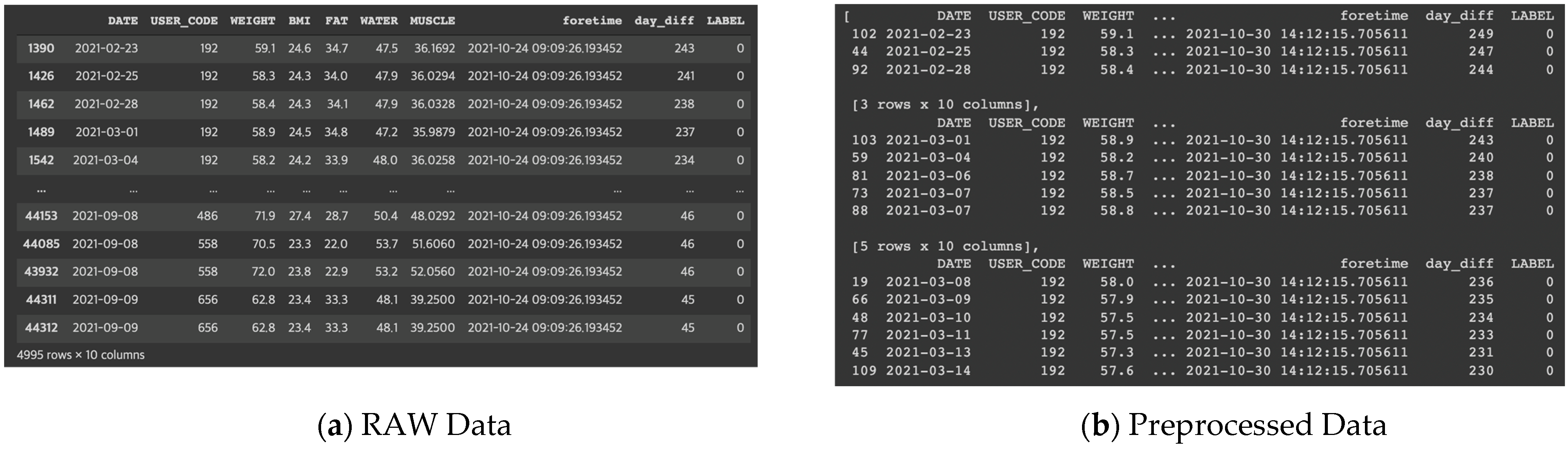
2.1. Data Preparation

First, raw data is converted into weekly data, starting with a data conversion, which converts the raw data (life log) of the wearable device into weekly data. An example of data conversion is presented in Figure 1. The reason for converting the raw data into weekly data is to take advantage of the small daily variability in the body weight data and to reflect periodicity and changes over time.
Second, we observe the average body weight per a week: due to the small daily variability in body weight, the weekly average body weight has little difference from the normal value for each day of the week. Therefore, the weekly average body weight value could be a criterion for determining when there is an abnormal value for the body weight data on the days of the week. For example, if a user weighs about 64 kg on Tuesday and about 63.8 kg on Wednesday, but weighs 70 kg on Friday, the probability of Friday’s weight value being an outlier is very high. On the other hand, if the weekly average weight value changes from 65 kg to 70 kg over a long time, it is considered normal weight. For example, suppose a user has an average body weight value of 65 kg on week 1 and an average body weight value of 70 kg on week 5. From the perspective of the 1st week data, the 5th week data is an abnormal value, but it is the weight value of a user who has gained body weight normally. Since the weight can have periodicity and is a value that changes with time, we determine whether a value is abnormal based on the calculated weekly average body weight value. This method reflects the change over time, so that the abnormal value can be determined more accurately.

2.2. Solution for the Problem of Outlier Class Imbalance

This study tried to solve the outlier class imbalance by generating outliers of various sizes. First. we generate outliers as much as the ratio of the number of outliers to the total number of data sets. In addition, the performance of the prediction algorithm can be improved by optimizing the outlier ratio by generating as many outliers as necessary according to the set number. In this study, the ratio was set to 10% outliers; both the study on the outlier ratio [42,43] and the study [44] that showed high accuracy when set to 10% were referred to. In addition, the data set was built on a daily basis and consists of about 100 individual data, so it is necessary to have at least one outlier data out of 10 days to determine the weekly trend, and it was expected that there should be at least 10 individual outlier data. It was judged that this can be optimized according to the data set.

2.3. Two Outliers Generation Methods

We propose two ways for generating outliers. When an outlier is generated by a single method or a single probability distribution, the number of generated outliers may be limited and the range of values of the outlier may be limited.
The first method generates outliers by adding search and noise to the original data set based on a uniform distribution, producing half the total number of outliers. Specifically, outliers are created by retrieving and extracting data from the original data set based on randomly drawn values from an established uniform distribution, adding noise, and replacing them with normal body weight values. Searching in the original data set allows one to replace with data that is as close to real data as possible. A problem that can occur when generating data virtually based on body weight is that it may be difficult to generate body variables other than body weight, such as FAT, WATER, and MUSCLE, in response to the appropriately generated body weight value. For example, it may be difficult to know the FAT value, WATER value, and MUSCLE value corresponding to a user weighing 78 kg immediately. When data points are retrieved by searching for data near 78 kg of weight in real data, the values of other variables can also be imported. This method has the advantage of generating outliers quickly and with realistic data. In other words, the values of other variables such as FAT and WATER can be imported from the actual data points, and more realistic outliers can be created by adding noise to them. When extracting random values, we use a uniform distribution so the lower and upper limits of the extracted values can be adjusted by setting the range.
The second method we used to generate the remaining half of the outliers to was the difference in probability distribution based on sex. This method reflects the physical differences between men and women in the normal distribution. Most variables in nature, such as height and blood pressure, are normally distributed. We therefore expect body weight also follows a normal distribution. In addition, the normal distribution was selected because it has the advantage of being able to extract data near a random but controllable mean by reducing the deviation.
Each generation method is described in detail below. In this study, the method of searching in the original data set is called the search module method (Section 2.3.1), and the method using the bimodal probability distribution reflecting sexual dimorphism is called the generation module method (Section 2.3.2).

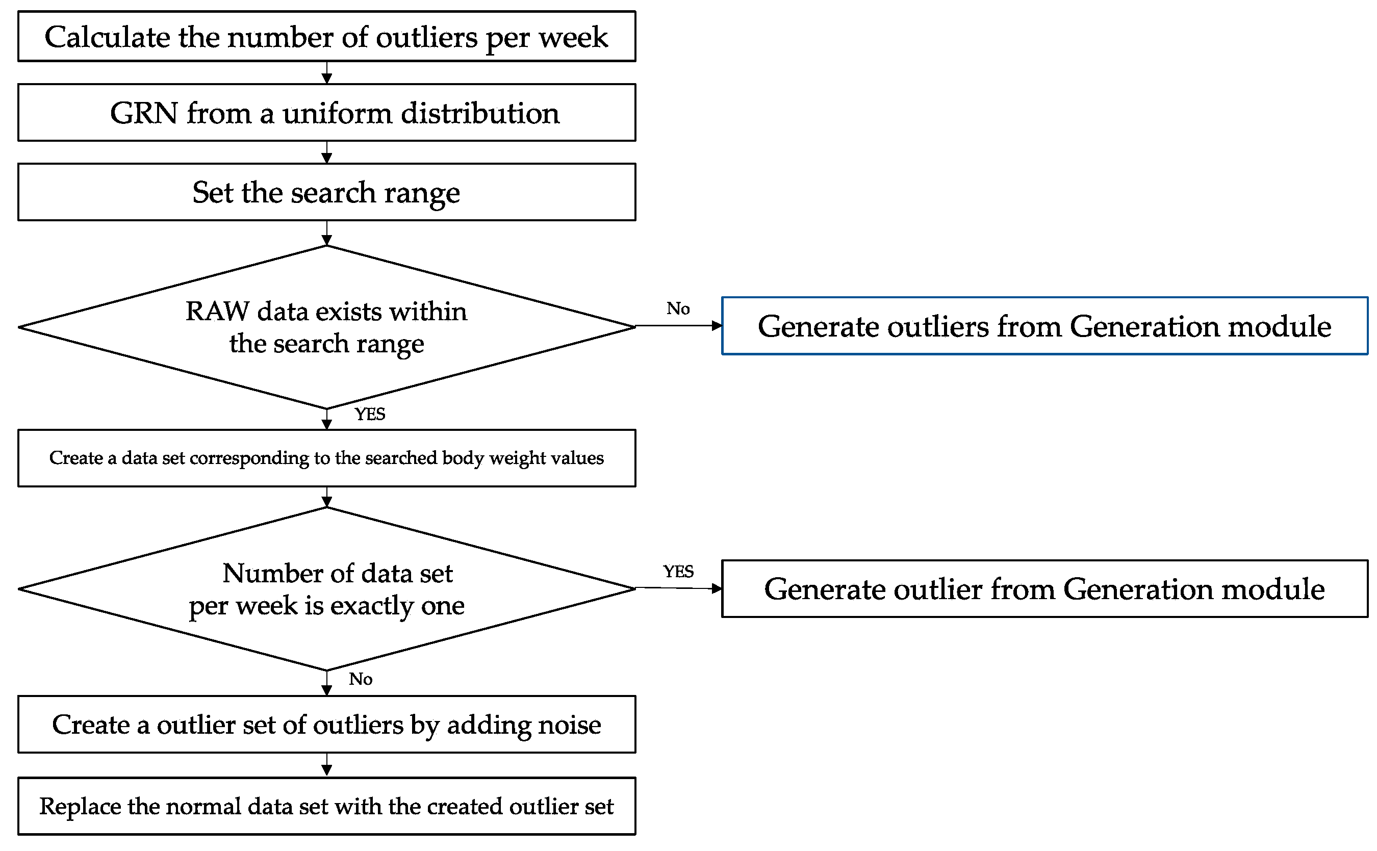
2.3.1. Search Module Method

The search module has a search criterion and a search scope. The search criterion is a value randomly extracted from a uniform distribution in the range of 40 kg or more and 120 kg or less. The values 40 kg and 120 kg are the minimum and maximum values of the original data set, respectively. The minimum and maximum values could be changed depending on the data set used. The search range was created based on the extracted search criterion value. After that, a random number was extracted from the uniform distribution on (0, 2), and we defined the upper limit to be the search criterion value + random number, and the lower limit as the search criterion value—the random number. Next, the searched values were extracted from the entire data set, and an outlier was generated by randomly extracting one of them. We proceeded with each of the search criteria and the search range because if you simply search with the search criteria, there is a high probability that the entire dataset does not have the same value as the search criteria. By adding a search range, it is possible to search in a slightly wider range while being similar to the search criterion value, thereby increasing the search probability. If it is not in the corresponding range, it is not in the original dataset, so the search is not performed. This does mean that the number of outliers generated may be insufficient; the remainder were added from the second module, the generation module. Figure 2 shows the overall flow for the search module.
  • Set the search range (GRN − RN, GRN + RN) based on the random number (GRN) generated with a uniform distribution of (40 kg, 120 kg).
    • RN is set as a real value in the range (0, 2).
  • Search and extract all values in the search range from all RAW data sets within the search range.
    • If there is no searched data, the generation module creates the remaining required outliers.
  • Create a data set by finding the BMI, FAT, WATER, and MUSCLE values corresponding to the searched body weight values.
  • Create a set of outliers by adding noise corresponding to each variable of the data set created in 3. The noise of each variable is summarized in Table 1.
  • The number of preset outliers is converted into the number of weekly generations.
  • Obtain an index for the day of the week according to the number of generations per week and replace the corresponding normal data with an outlier table.
  • Repeat steps 1–6 for each week to generate outliers by substituting them.

2.3.2. Generation Module Method

The remaining half of the number of outliers were generated using the bimodal probability distribution reflecting sexual dimorphism. BMI, FAT, MUSCLE, and WATER values corresponding to the calculated body weight criterion values were also generated according to sex. Figure 3 shows the overall flow for the generation module.
  • The generation module creates the number of outliers to be generated, minus the total number of outliers generated by the search module.
  • Divide the number of outliers to be generated in the generation module by the number of weeks to calculate the number to be generated per week.
  • Excluding the days selected in the search module, the number of day indices to be created per week is extracted.
  • The average of the normal distribution was obtained by multiplying the weekly average weight calculated for each week by an arbitrary ratio of 1.1, and the mean standard deviation was set to “2”. The mean standard deviation, “2”, may change depending on data characteristics. Here, the reason for multiplying by 1.1 was to minimize distortion due to the difference in weight values. For example, 5 kg for a 50 kg user and 5 kg for an 80 kg user is the same 5 kg but feels different. Therefore, rather than modifying the weight by addition, we applied a multiplicative scaling to increase fairness.
    Average(A) = average + (average × random ratio), which ratio = 0.1
    Standard deviation(S) = ± 2
  • Generate one body weight (BW) randomly from the graph (A, S) of normal distribution created in step 1.
  • Based on the weight reference value obtained in step 5, if it is greater than 70, it is assumed that it is a man, and if it is less than 70, it is created separately.The reason for this setting is that, as a result of the data set EDA (Exploratory Data Analysis), the maximum value of women’s weight was less than 70.
6-1. For males, BMI was calculated by setting the height to 1.73 m, the average male height in Korea, and randomly extracting WATER and FAT from a uniform distribution in the ranges of (50, 65), (17, 32), respectively, then computing the MUSCLE value by subtracting FAT from the reference body weight value. Finally, random noise corresponding to each variable was added. (See Table 1).
6-2. For females, BMI was calculated by setting the height to 1.61 m, the average male height in Korea, and randomly extracting WATER and FAT from a uniform distribution in the ranges of (45, 60) and (15, 30), respectively, then computing the MUSCLE value by subtracting FAT from the reference body weight value. Finally, random noise corresponding to each variable was added (See Table 1). The uniform distribution range of each variable was set based on the minimum and maximum values of each variable based on the data set.
7.
Create an outlier by replacing the outlier data obtained in 6-1 or 6-2 with the normal value of the selected day index.
8.
Repeat steps 1–7 for each week to generate outliers.
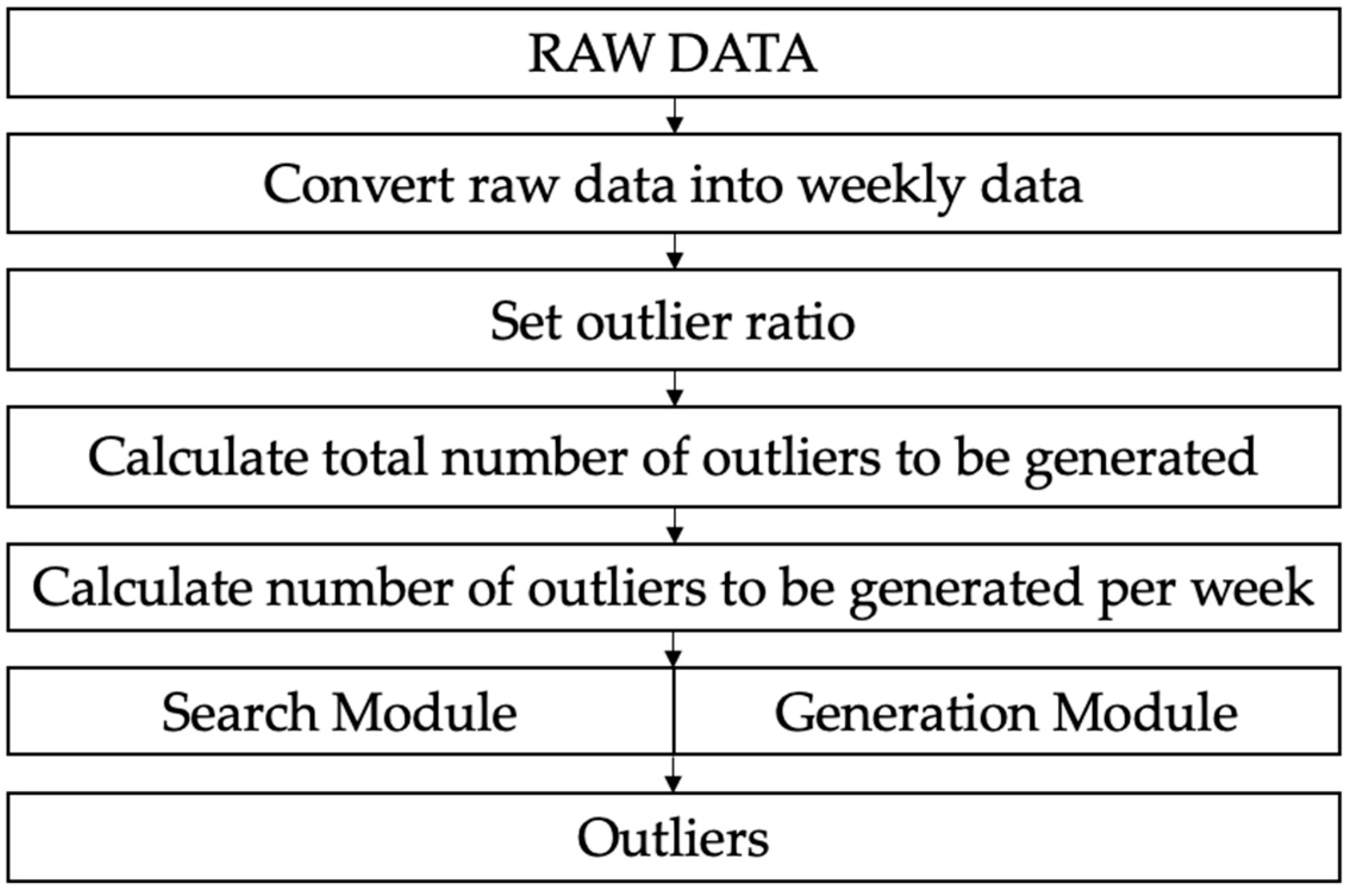
2.3.3. Summary

To summarize, the proposed two outlier generation algorithms generate as many outliers as the ratio of the number of outliers to the total size of the data set in advance. Half of the outliers to be generated are generated by the search module, and the other half are generated by the generation module. The search module searches for data in the entire data set based on the reference value obtained from the uniform distribution, and adds noise based on the searched data point to create an outlier. The generation module uses a normal distribution based on the average body values according to sex to generate the other half of the outliers. If there is no searchable data for the search module, the generation module will create additional outliers to compensate. Figure 2 shows the overall algorithm flow. Figure 4 shows the overall algorithm flow.
  • Convert all general time series data (RAW data) into weekly data.
  • Set the pre-set ratio of the number of outliers to the total number of data (“outlier value generation ratio”)
  • Calculate the total number of outliers to be generated through the outlier generation ratio.
  • Calculate the number of outliers to be generated per week by dividing the total number of outliers by the number of weeks.
  • For each week, half of the outliers are generated by the search module and the other half are generated by the generation module. At this time, the generation module generates as many outliers as the number of outliers that were not generated by the search module if it did not satisfy the execution condition.

3. Results

Lifelogs were collected through a Samsung Galaxy Watch active 2, smart scale (IoT device) and mobile application (GIVita app), and the collected information was stored in the database. Specifically, the users lifelog and user information that are generated in real time are collected. Continuous lifelogs such as sleep, steps, and weight are generated through a smart watch and a smart scale and transmitted to a mobile application. It receives the lifelog and user information sent from the mobile application and sends it to the lifelog DB to store the data. Among the data, 59 users (data) have been used with 124 rows of four months or more. Outliers accounted for approximately 1.06% of the total. Table 2 summarizes the detailed description of the body weight data set, and Table 3 explains user information and derived variables.
To verify the effectiveness of the proposed algorithm, this study validates generated data quality using several supervised learning classification algorithms: SVM (Support Vector Machine) [45], XGBoost (Extreme Gradient Boosting) [46] and CatBoost (Categorical Boosting) [47]. It validates the data generated and augmented by SMOTE, SMOTE + ENN), SMOTE + TOMEK, CTGAN, and our proposed algorithm.
Since the number of hyperparameter combinations of the machine learning algorithm used in this study is large and the performance difference is large depending on the tuned parameters, it was optimized using a Bayesian-based hyperopt frame [48] for effective tuning. A hyperopt frame consists of four functions: (1) Search space: it is a probabilistic search space and has various functions to specify the range of input parameters. (2) Objective function: a minimization function that receives hyperparameter values from the search space as input and returns a loss. (3) Fmin: an optimization function that iterates over a set of different algorithms and hyperparameters and then minimizes the objective function, and (4) Trials object: used to hold all hyperparameters, losses and other information. In addition, the entire data was divided in an 8:2 ratio where 80% of the data is used for algorithm training, and 20% of the data is test data.
In this study, F1 score, and AUC (Area Under the Receiver operating characteristic) were used as performance indicators, each of which is summarized in the following Table 4 and Table 5.
In Table 4 and Table 5 above, our proposed algorithm performed the best in both F1 Score and AUC.
To summarize the results of the experiment, our proposed method outperforms both, analyzing the raw data without preprocessing and analyzing the previous methods. Our proposed method outperforms in both F1 score and AUC: for F1 score, 0.987 with XGBOOST, and 0.987 with CATBOOST (refer to Table 4); and for AUC score, 0.986 in XGBOOST, and 0.998 in CATBOOST (refer to Table 5). This shows that augmenting the outlier data in a way that reflects the time information of periodic variability is more effective in detecting outliers in characteristics of body weight data than the traditional SMOTE method and the latest VAE and CTGAN data augmentation methods.

4. Discussion

Most of the existing studies defined an outlier as an outlier only when it was signficantly different from the normal value, and only pre-processing methodologies for related outliers were presented. There are not enough studies on cases where there is no significant difference between the outlier and the normal value. As the importance of body weight in the lifelog is highlighted, it is important for digital healthcare research, but research on the preprocessing methodology for body weight is also highlighted. However, there are also not enough of specialized preprocessing studies for data with periodicity and small daily variability, such as body weight data. Therefore, this study proposes an outlier generation method suitable for the characteristics of body weight lifelog data.
To demonstrate the superiority of the proposed algorithm, lifelogs of 59 users were collected over 4 months. In these logs, 1.06% of the total data are outliers. The experiments showed that the proposed method performed better than using the traditional SMOTE method and the latest CTGAN method. Specifically, both F1 scores and AUC scores were improved in the SVM, XGBOOST, and CATBOOST algorithms, and significantly improved compared to no preprocessing.
However, this study had potential instability limitations in data collection caused by external factors such as battery shortage and network instability that may occur in the Galaxy Watch environment. This is expected to be resolved through more sophisticated preprocessing. For example, in the case of sleep, there is a way to reduce distortion by analyzing individual sleep cycles and generating derived variables.

5. Conclusions

Our proposed method reduces the level of data imbalance and improves analytic accuracy by generating outliers based on time information in consideration of the periodicity and variability of the body weight lifelog. Through the method, the problem of body weight outlier class imbalance is solved, and the time-dependent characteristics of daily variability and periodicity of weight data can be reflected. Specifically, outliers are generated through the search module and generation module, which can solve the problem of weight outlier class imbalance and reflect the time-dependent characteristics of small daily variability and periodicity of weight data: (1) For body weight data with small daily variability and periodicity, processing class imbalance by integrating time information would be more effective than data augmentation by learning all data in general. (2) It can be effective to detect outliers by generating outliers and then providing data to a machine learning algorithm to detect the outliers, which is an effective data preprocessing method for detecting actual weight anomalies. (3) Even an outlier that does not differ significantly from the normal value can be effectively detected through the relevant preprocessing method.
Through the experiments of this study, it was confirmed that the proposed outlier generation method improved the performance of machine learning anomaly detection the most. This suggests that a preprocessing method for generating outliers specialized for body weight data is important, and since performance is greatly improved compared to no preprocessing, it suggests that a preprocessing methodology suitable for data characteristics is important and would improve performance. A study on skin lesion images data that improved deep learning performance using an augmentation methodology [49], a study that applied and compared various preprocessing methodologies specific to univariate volatile time series data [50], and a comparative study of preprocessing on medical data [51] are all consistent with the conclusion of this study that it is important to preprocess according to the characteristics of the data and can improve performance. Therefore, preprocessing suitable for the characteristics of the data is important.
We have a plan to apply our proposed method with not only lifelogs but also various industries in the future. It is expected to be applicable to a data set that is not volatile and occurs periodically. For example, we plan to further verify that it can be applied in financial industries such as stocks, or in processes where there is a fine adjustment of values. In addition, optimization research on the noise in each variable will be conducted together.

Author Contributions

Conceptualization, J.K. and M.P.; data curation, J.K.; formal analysis, J.K.; funding acquisition, M.P.; methodology, J.K. and M.P.; supervision, M.P.; validation, J.K.; visualization, J.K.; writing—original draft preparation, J.K. and M.P.; writing—review and editing, M.P. All authors have read and agreed to the published version of the manuscript.

Funding

This work was supported by a research grant from Seoul Women’s University (2021-0423).

Institutional Review Board Statement

Not applicable.

Informed Consent Statement

Informed consent was obtained from all subjects involved in the study.

Data Availability Statement

Not applicable.

Conflicts of Interest

The authors declare no conflict of interest.

References

  1. Lee, Y.-J.; Ko, Y.S. A Lifelog Common Data Reference Model for the Healthcare Ecosystem. Knowl. Manag. Res. 2018, 19, 149–170. [Google Scholar]
  2. Qi, J.; Yang, P.; Hanneghan, M.; Latham, K.; Tang, S. Uncertainty Investigation for Personalised Lifelogging Physical Activity Intensity Pattern Assessment with Mobile Devices. In Proceedings of the 2017 IEEE International Conference on Internet of Things (iThings) and IEEE Green Computing and Communications (GreenCom) and IEEE Cyber, Physical and Social Computing (CPSCom) and IEEE Smart Data (SmartData), Exeter, UK, 21–23 June 2017; pp. 871–876. [Google Scholar]
  3. Yang, P.; Stankevicius, D.; Marozas, V.; Deng, Z.; Liu, E.; Lukosevicius, A.; Dong, F.; Xu, L.; Min, G. Lifelogging Data Validation Model for Internet of Things Enabled Personalized Healthcare. In IEEE Transactions on Systems, Man, and Cybernetics: Systems; IEEE: Manhattan, NY, USA, 2018; Volume 48, pp. 50–64. [Google Scholar] [CrossRef] [Green Version]
  4. Park, M.S. Application and Expansion of Artificial Intelligence Technology to Healthcare. J. Bus. Converg. 2021, 6, 101–109. [Google Scholar] [CrossRef]
  5. Zheng, Y.; Manson, J.E.; Yuan, C. Associations of Weight Gain from Early to Middle Adulthood with Major Health Outcomes Later in Life. JAMA 2017, 318, 255–269. [Google Scholar] [CrossRef] [PubMed]
  6. Wilding, J. The importance of weight management in type 2 diabetes mellitus. Int. J. Clin. Pract. 2014, 68, 682–691. [Google Scholar] [CrossRef] [PubMed] [Green Version]
  7. Ades, P.A.; Savage, P.D. Potential Benefits of Weight Loss in Coronary Heart Disease. Prog. Cardiovasc. Dis. 2014, 56, 448–456. [Google Scholar] [CrossRef] [PubMed]
  8. Blumenthal, J.A.; Sherwood, A.; Gullette, E.C.; Babyak, M.; Waugh, R.; Georgiades, A.; Hinderliter, A. Exercise and weight loss reduce blood pressure in men and women with mild hypertension: Effects on cardiovascular, metabolic, and hemodynamic functioning. Arch. Intern. Med. 2000, 160, 1947–1958. [Google Scholar] [CrossRef] [Green Version]
  9. Blumenthal, J.A.; Babyak, M.A.; Hinderliter, A. Effects of the DASH Diet Alone and in Combination with Exercise and Weight Loss on Blood Pressure and Cardiovascular Biomarkers in Men and Women with High Blood Pressure: The ENCORE Study. Arch Intern Med. 2010, 170, 126–135. [Google Scholar] [CrossRef]
  10. Pak, M.; Lindseth, G. Risk factors for cholelithiasis. Gastroenterol. Nurs. 2016, 39, 297–309. [Google Scholar] [CrossRef]
  11. Demark-Wahnefried, W.; Campbell, K.L.; Hayes, S.C. Weight management and its role in breast cancer rehabilitation. Cancer 2012, 118, 2277–2287. [Google Scholar] [CrossRef] [Green Version]
  12. Ali, S.; Khusro, S.; Khan, A.; Khan, H. Smartphone-Based Lifelogging: Toward Realization of Personal Big Data. In Information and Knowledge in Internet of Things; Guarda, T., Anwar, S., Leon, M., Mota Pinto, F.J., Eds.; Springer: Cham, Switzerland, 2022. [Google Scholar]
  13. Choi, J.; Choi, C.; Ko, H.; Kim, P. Intelligent Healthcare Service Using Health Lifelog Analysis. J. Med. Syst. 2016, 40, 188. [Google Scholar] [CrossRef]
  14. Kim, J.W.; Lim, J.H.; Moon, S.M.; Jang, B. Collecting Health Lifelog Data from Smartwatch Users in a Privacy-Preserving Manner. IEEE Trans. Consum. Electron. 2019, 65, 369–378. [Google Scholar] [CrossRef]
  15. Deng, Z.; Zhao, Y.; Parvinzamir, F.; Zhao, X.; Wei, S.; Liu, M.; Zhang, X.; Dong, F.; Liu, E.; Clapworthy, G. MyHealthAvatar: A Lifetime Visual Analytics Companion for Citizen Well-being. In International Conference on Technologies for E-Learning and Digital Entertainment; Springer: Cham, Switzerland, 2016; pp. 345–356. [Google Scholar]
  16. Ni, J.; Chen, B.; Allinson, N.M.; Ye, X. A hybrid model for predicting human physical activity status from lifelogging data. Eur. J. Oper. Res. 2019, 281, 532–542. [Google Scholar] [CrossRef] [Green Version]
  17. Kim, J.Y.; Lee, J.S.; Park, M.S. Analysis of Lifelong for Health of Middle-Aged Men by Using Machine Learning Algorithm. J. Korean Inst. Ind. Eng. 2021, 47, 504–513. [Google Scholar]
  18. Chung, C.F.; Cook, J.; Bales, E.; Zia, J.; Munson, S.A. More Than Telemonitoring: Health Provider Use and Nonuse of Life-Log Data in Irritable Bowel Syndrome and Weight Management. J. Med. Internet Res. 2015, 17, e203. [Google Scholar] [CrossRef] [Green Version]
  19. Muruti, G.; Rahim, F.; Ibrahim, Z.A. A Survey on Anomalies Detection Techniques and Measurement Methods. In Proceedings of the 2018 IEEE Conference on Application, Information and Network Security (AINS), Langkawi, Malaysia, 21–22 November 2018. [Google Scholar] [CrossRef]
  20. Wang, H.; Bah, M.J.; Hammad, M. Progress in Outlier Detection Techniques: A Survey. IEEE Access 2019, 7, 107964–108000. [Google Scholar] [CrossRef]
  21. Berthoud, H.R.; Morrison, C.D.; Münzberg, H. The obesity epidemic in the face of homeostatic body weight regulation: What went wrong and how can it be fixed? Physiol. Behav. 2020, 222, 112959. [Google Scholar] [CrossRef]
  22. Chawla, N.V.; Bowyer, K.W.; Hall, L.O.; Kegelmeyer, W.P. SMOTE: Synthetic minority over-sampling technique. J. Artif. Intell. Res. 2002, 16, 321–357. [Google Scholar] [CrossRef]
  23. Luengo, J.; Fernández, A.; García, S.; Herrera, F. Addressing data complexity for imbalanced data sets: Analysis of SMOTE-based oversampling and evolutionary undersampling. Soft Comput. 2010, 15, 1909–1936. [Google Scholar] [CrossRef]
  24. Wilson, D.L. Asymptotic properties of nearest neighbor rules using edited data. IEEE Trans. Syst. Man Cybern. 1972, 3, 408–421. [Google Scholar] [CrossRef] [Green Version]
  25. Vuttipittayamongkol, P.; Elyan, E. Neighbourhood-based undersampling approach for handling imbalanced and overlapped data. Inf. Sci. 2020, 509, 47–70. [Google Scholar] [CrossRef]
  26. Batista, G.E.; Prati, R.C.; Monard, M.C. A study of the behavior of several methods for balancing machine learning training data. ACM SIGKDD Explor. Newsl. 2004, 6, 20–29. [Google Scholar] [CrossRef]
  27. Tomek, I. Two Modifications of CNN. IEEE Trans. Syst. Man Cybern. 1976, 6, 769–772. [Google Scholar]
  28. Ramentol, E.E.; Caballero, Y.; Bello, R. SMOTE-RSB*: A hybrid preprocessing approach based on oversampling and undersampling for high imbalanced data-sets using SMOTE and rough sets theory. Knowl. Inf. Syst. 2012, 33, 45–265. [Google Scholar] [CrossRef]
  29. Wang, S.; Li, Z.; Chao, W.; Cao, Q. Applying adaptive over-sampling technique based on data density and cost-sensitive SVM to imbalanced learning. In Proceedings of the 2012 International Joint Conference on Neural Networks (IJCNN), Brisbane, QLD, Australia, 10–15 June 2012; pp. 1–8. [Google Scholar]
  30. Xu, L.; Skoularidou, M.; Cuesta-Infante, A.; Veeramachaneni, K. Modeling tabular data using conditional gan. arXiv 2019, arXiv:1907.00503. [Google Scholar]
  31. Bourou, S.; El Saer, A.; Velivassaki, T.H.; Voulkidis, A.; Zahariadis, T. A Review of Tabular Data Synthesis Using GANs on an IDS Dataset. Information 2021, 12, 375. [Google Scholar] [CrossRef]
  32. Maldonado, S.; López, J.; Vairetti, C. An alternative SMOTE oversampling strategy for high-dimensional datasets. Appl. Soft Comput. 2018, 76, 380–389. [Google Scholar] [CrossRef]
  33. Bowles, C.; Chen, L.; Guerrero, R.; Bentley, P.; Gunn, R.; Hammers, A.; Rueckert, D. GAN augmentation: Augmenting training data using generative adversarial networks. arXiv 2018, arXiv:1810.10863. [Google Scholar]
  34. Nnamoko, N.; Korkontzelos, I. Efficient treatment of outliers and class imbalance for diabetes prediction. Artif. Intell. Med. 2020, 104, 101815. [Google Scholar] [CrossRef]
  35. Loyola-González, O.; Martínez-Trinidad, J.F.; Carrasco-Ochoa, J.A.; García-Borroto, M. Effect of class imbalance on quality measures for contrast patterns: An experimental study. Inf. Sci. 2016, 374, 179–192. [Google Scholar] [CrossRef]
  36. Kuhn, M.; Johnson, K. Remedies for severe class imbalance. In Applied Predictive Modeling; Springer: New York, NY, USA, 2013; pp. 419–443. [Google Scholar]
  37. Racette, S.B.; Weiss, E.P.; Schechtman, K.B.; Steger-May, K.; Villareal, D.T.; Obert, K.A.; Washington University School of Medicine CALERIE Team. Influence of weekend lifestyle patterns on body weight. Obesity 2008, 16, 1826–1830. [Google Scholar] [CrossRef]
  38. Orsama, A.L.; Mattila, E.; Ermes, M.; van Gils, M.; Wansink, B.; Korhonen, I. Weight rhythms: Weight increases during weekends and decreases during weekdays. Obes. Facts 2014, 7, 36–47. [Google Scholar] [CrossRef] [PubMed]
  39. Madden, K.M. The Seasonal Periodicity of Healthy Contemplations About Exercise and Weight Loss: Ecological Correlational Study. JMIR Public Health Surveill. 2017, 3, e92. [Google Scholar] [CrossRef] [PubMed]
  40. Turicchi, J.; O’Driscoll, R.; Horgan, G.; Duarte, C.; Palmeira, A.L.; Larsen, S.C.; Stubbs, J. Weekly, seasonal and holiday body weight fluctuation patterns among individuals engaged in a European multi-centre behavioural weight loss maintenance intervention. PLoS ONE 2020, 15, e0232152. [Google Scholar] [CrossRef] [PubMed]
  41. Moreno, J.P.; Johnston, C.A.; Chen, T.A.; O’Connor, T.A.; Hughes, S.O.; Baranowski, J.; Baranowski, T. Seasonal variability in weight change during elementary school. Obesity 2015, 23, 422–428. [Google Scholar] [CrossRef]
  42. Xia, Y.; Cao, X.; Wen, F.; Hu, G.; Sun, J. Learning Discriminative Reconstructions for Unsupervised Outlier Removal. In Proceedings of the 2015 IEEE International Conference on Computer Vision (ICCV), Santiago, Chile, 7–13 December 2015; pp. 1511–1519. [Google Scholar] [CrossRef]
  43. Gao, Y.; Ma, J.; Zhao, J. A robust and outlier-adaptive method for non-rigid point registration. Pattern Anal. Appl. 2013, 17, 379–388. [Google Scholar] [CrossRef]
  44. Mouret, F.; Albughdadi, M.; Duthoit, S.; Kouamé, D.; Rieu, G.; Tourneret, J.-Y. Outlier Detection at the Parcel-Level in Wheat and Rapeseed Crops Using Multispectral and SAR Time Series. Remote Sens. 2021, 13, 956. [Google Scholar] [CrossRef]
  45. Noble, W.S. What is a support vector machine? Nat. Biotechnol. 2006, 24, 1565–1567. [Google Scholar] [CrossRef]
  46. Chen, T.; Guestrin, C. Xgboost: A scalable tree boosting system. In Proceedings of the 22nd Acm Sigkdd International Conference on Knowledge Discovery and Data Mining, San Francisco, CA, USA, 13–17 August 2016; pp. 785–794. [Google Scholar]
  47. Dorogush, A.V.; Ershov, V.; Gulin, A. CatBoost: Gradient boosting with categorical features support. arXiv 2018, arXiv:1810.11363. [Google Scholar]
  48. Bergstra, J.; Yamins, D.; Cox, D.D. Hyperopt: A Python Library for Optimizing the Hyperparameters of Machine Learning Algorithms. In Proceedings of the 12th Python in Science Conference, Austin, TX, USA, 24–29 June 2013; p. 20. [Google Scholar]
  49. Ayan, E.; Ünver, H.M. Data augmentation importance for classification of skin lesions via deep learning. In Proceedings of the 2018 Electric Electronics, Computer Science, Biomedical Engineerings’ Meeting (EBBT), Istanbul, Turkey, 18–19 April 2018; pp. 1–4. [Google Scholar] [CrossRef]
  50. Ranjan, K.G.; Prusty, B.R.; Jena, D. Review of preprocessing methods for univariate volatile time-series in power system applications. Electr. Power Syst. Res. 2021, 191, 106885. [Google Scholar] [CrossRef]
  51. Hassler, A.; Menasalvas, E.; García-García, F.J.; Rodríguez-Mañas, L.; Holzinger, A. Importance of medical data preprocessing in predictive modeling and risk factor discovery for the frailty syndrome. BMC Med. Inform. Decis. Mak. 2019, 19, 33. [Google Scholar] [CrossRef]
Figure 1. (a) Raw data collected from a wearable device; (b) Data set preprocessed per week. ‘day_diff’ indicates a derived variable. The value 249 means the number of days between the data collection time and the date of 2 October 2021, which has been taken as the standard in this study.
Applsci 12 04726 g001
Figure 2. The Search module: An outlier generation module based on data set exploration, this is a flowchart of the search module.
Applsci 12 04726 g002
Figure 3. The Generation module: this module uses a normal distribution based on gender physical differences.
Applsci 12 04726 g003
Figure 4. The overall algorithm for two methods: search module and generation module.
Applsci 12 04726 g004
Table 1. Description of the noise of each variable set to calculate different variables.
Data VariableVariable Description and Range
Random Noise for body weightNoise for search scope, any real value between (0, 2)
BMI NoiseNoise for BMI calculation, any real value between (0.5, 1.5)
Body Mass NoiseNoise for calculating body mass, any real value between (1.5, 3)
Muscle Mass NoiseNoise for muscle mass calculation, any real value between (0.5, 3)
Height NoiseUsed for BMI calculation with noise for the set height
FATAny real value between (17, 32) for men + body mass noise, and random real value between (15, 30) for women + body mass noise
MUSCLEWeight Value—Body Mass Value + Muscle Noise
Body Water NoiseNoise for body water calculation, any real value between (2.5, 3)
WeightWeight Value + Weight Noise from full RAW data
BMIWeight (kg)/(Height (m) + Height Noise)2 The height of 1.73 m for males and 1.61 m for females is the standard height used in calculations.
WaterAny real value between (50, 65) for male + body water noise, and random real value between (45, 60) for female + body water noise
Table 2. Variables and variable descriptions of dataset.
VariableDescription
DATEData Collection Date
WEIGHTUser’s Weight
FATUser’s Body Fat
MUSCLEUser’s Muscle Mass
USER_CODEUser’s Identification Code
BMIUser’s Weight
WATERUser’s Body Water
Table 3. Variables, derived variable, and variable descriptions of user information dataset.
VariableDescription
BIRTH_YEAR_MONTHUser’s date of birth and month
GENDERUser’s gender
USER_CODEUser’s identification code
HEIGHTUser’s height
HEIGHT_CATEGORIZE_10User’s height category in 10 cm increments from 160 cm to 190 cm
DAY_DIFFTo reflect the date information of the data point due to the difference in date days as 2 October 2021
LABELIt is a variable showing a normal value: 0 and an abnormal value: 1 and is used for performance evaluation.
Table 4. F1 score of the classification algorithm according to each data augmentation.
NoneSMOTESMOTE + ENNSMOTE + TOMEKCTGANProposed Algorithms
SVM0.2070.8780.8860.8280.8880.986
XGBoost0.2070.8180.8220.9680.8050.987
CatBoost0.3230.9650.9690.8880.9480.987
Table 5. AUC score of the classification algorithm according to each data augmentation.
NoneSMOTESMOTE + ENNSMOTE + TOMEKCTGANProposed Algorithms
SVM0.8120.9520.9560.9530.9360.995
XGBoost0.9380.9650.9680.9620.9380.986
CatBoost0.9900.9680.9920.9710.9830.998
Publisher’s Note: MDPI stays neutral with regard to jurisdictional claims in published maps and institutional affiliations.

