
Concept for Generating Energy Demand in Electric Vehicles with a Model Based Approach


Abstract
:1. Introduction
2. State of the Art
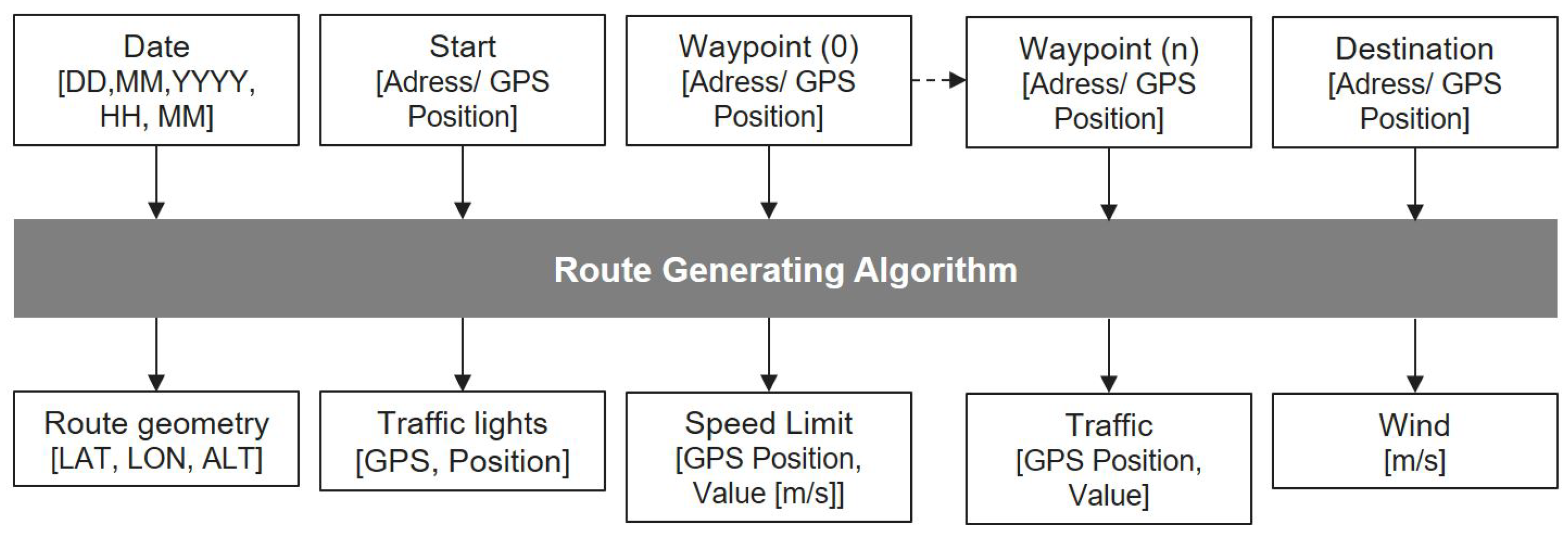
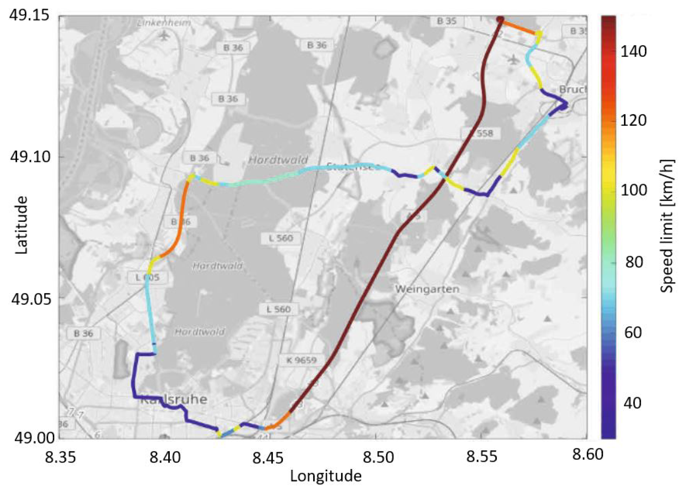
3. Route Data
4. Simulation and Model Environment
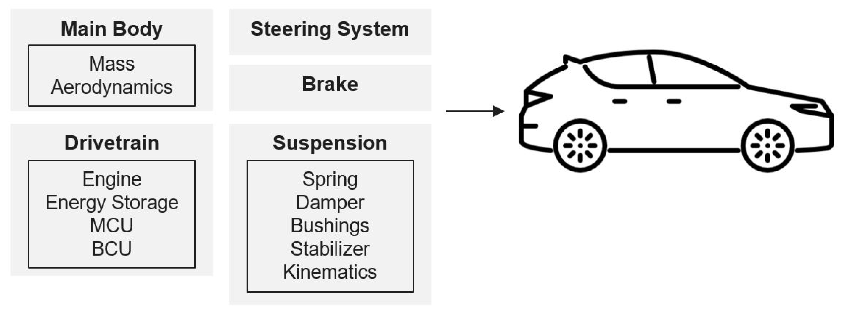
4.1. Vehicle Model
- -
- The main body, with information about the total mass and the aerodynamic behavior of the vehicle;
- -
- The steering system, which contains information about the ratio between the steering wheel angle (or steering wheel torque) and the steering rack displacement;
- -
- The suspension, with the components including the springs, dampers, bushings, and stabilizers and the kinematics of the chassis;
- -
- The drivetrain, which contains information about the engine, energy storage, motor control unit (MCU) and the battery control unit (BCU);
- -
- The brakes, with information about the possible deceleration of the vehicle.
4.1.1. Battery Model
4.1.2. Supercapacitor Model
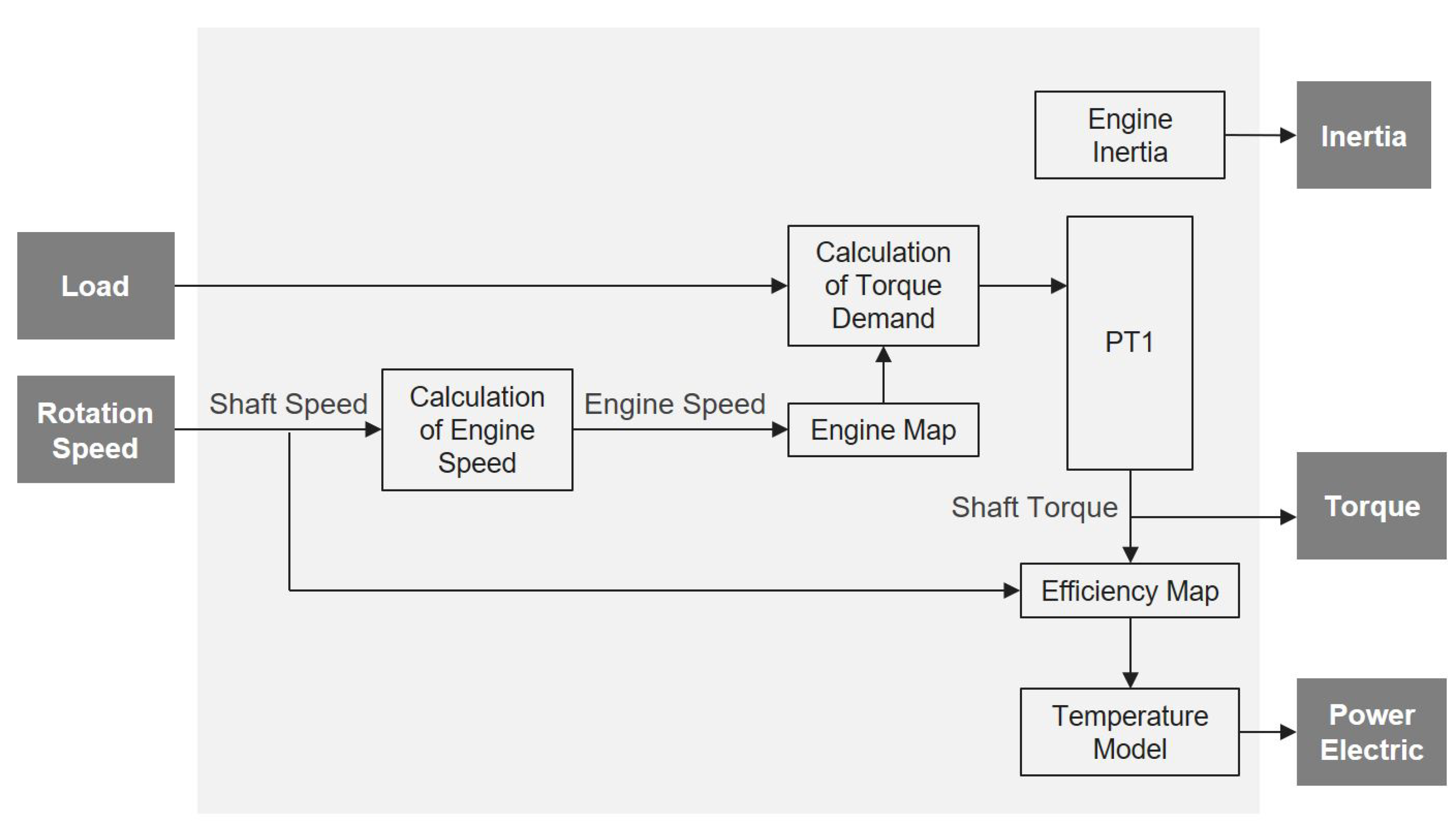
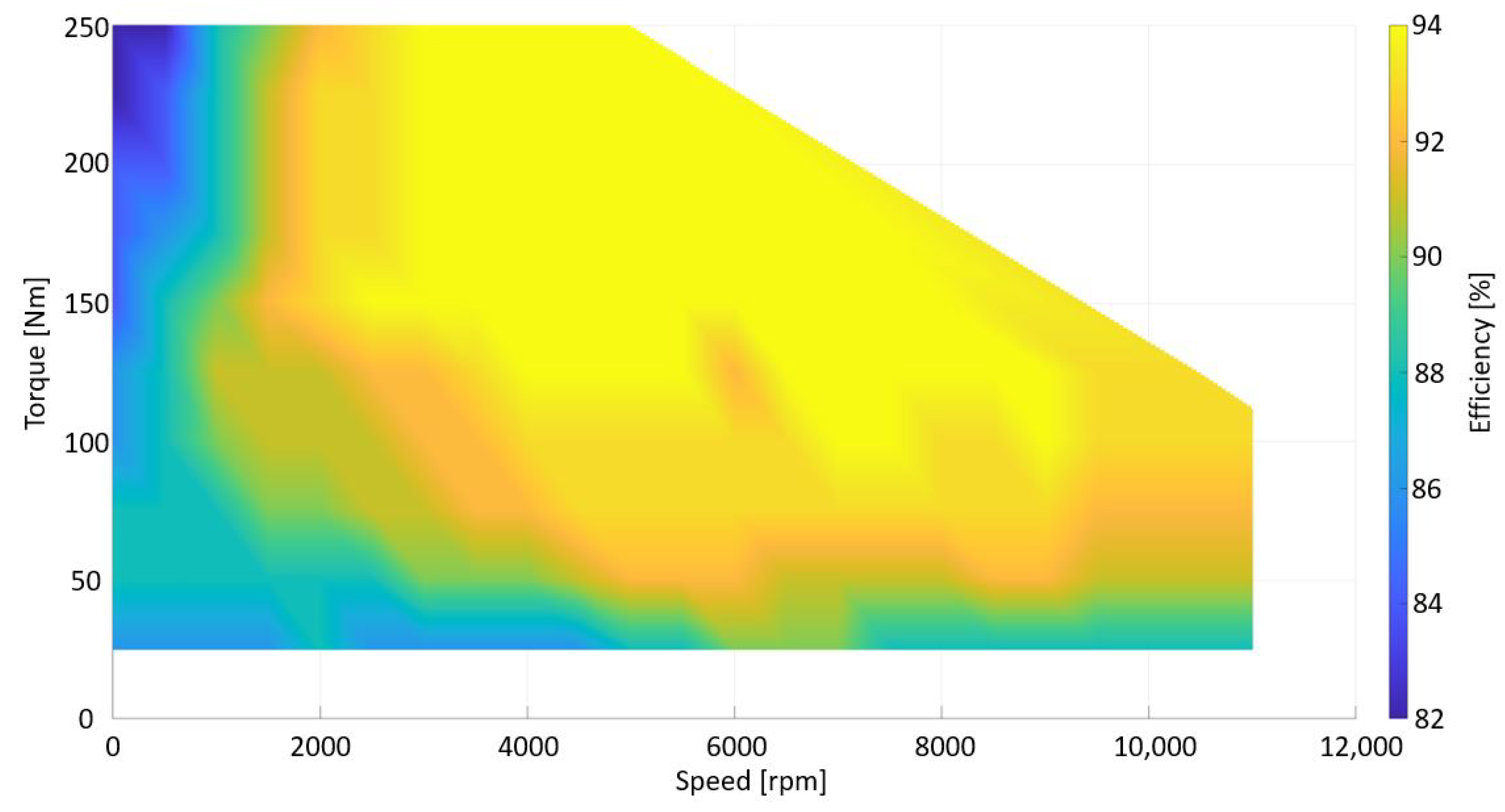
4.1.3. Drivetrain Model
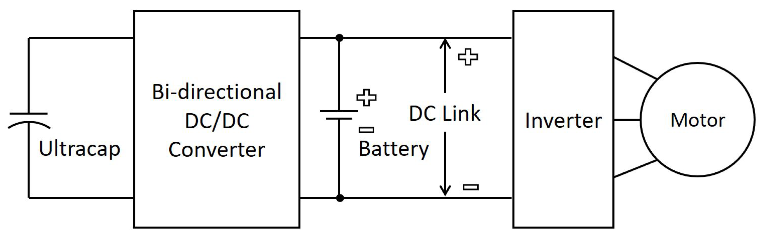
4.1.4. DC/DC Converter Model
- -
- Semiactive control strategies can be implemented;
- -
- The operating range of the energy storage components can be extended to improve the performance of the HESS;
- -
- It provides flexibility to reduce the size/voltage of some of the energy storage components.
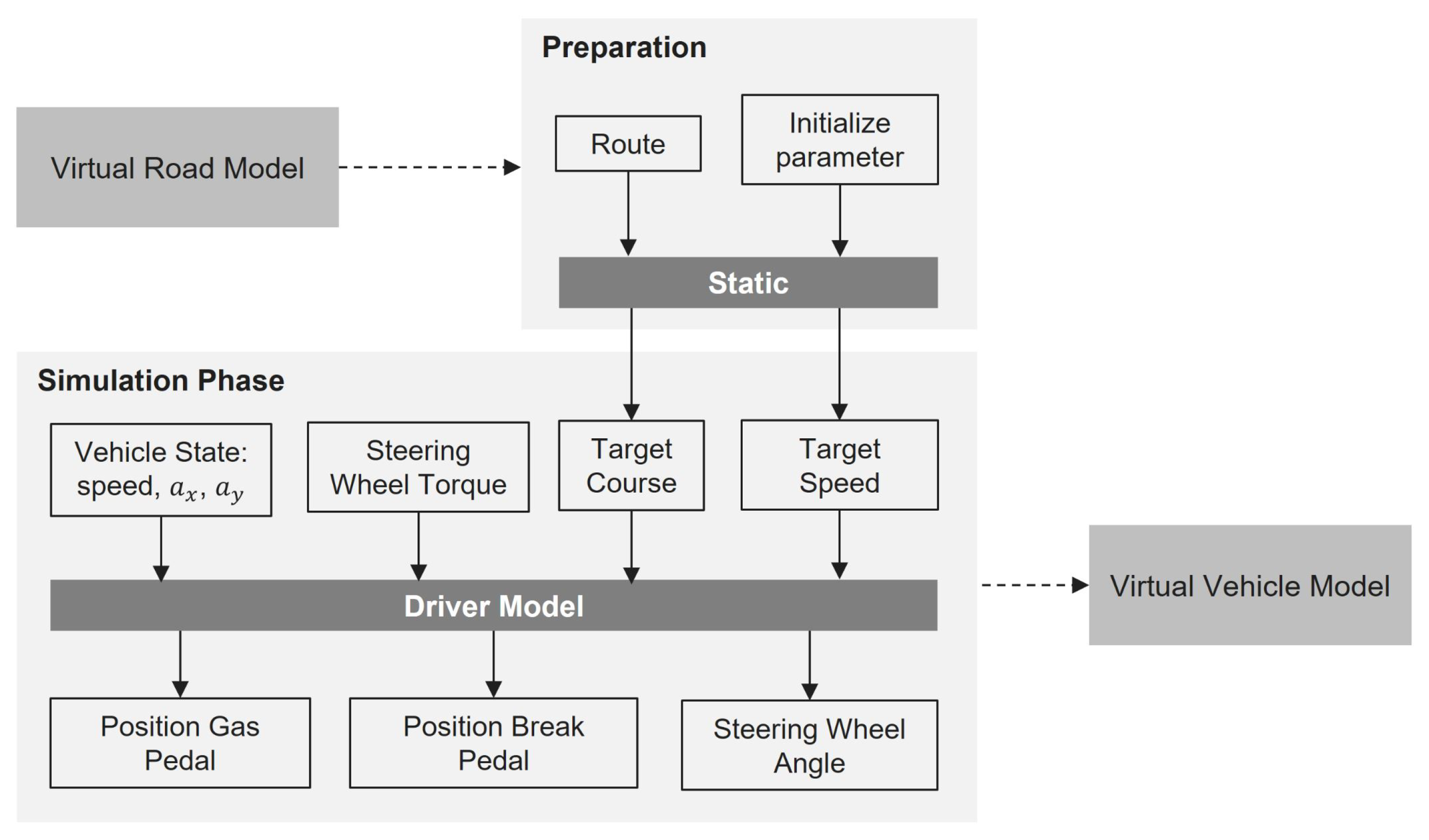
4.2. Adaptive Driver Model
- -
- Target course: Builds the course based on the input data. This is represented as a trajectory over a 2D surface by defining the x and y coordinates along a centerline (with a certain width). This form of mapping can be adjusted by the parameters previously set by the driver model, such as adjusting the ideal driving line. If this is set so that the driver model should use the entire width of the road (or only one lane), the model will adjust the centerline accordingly [38];
- -
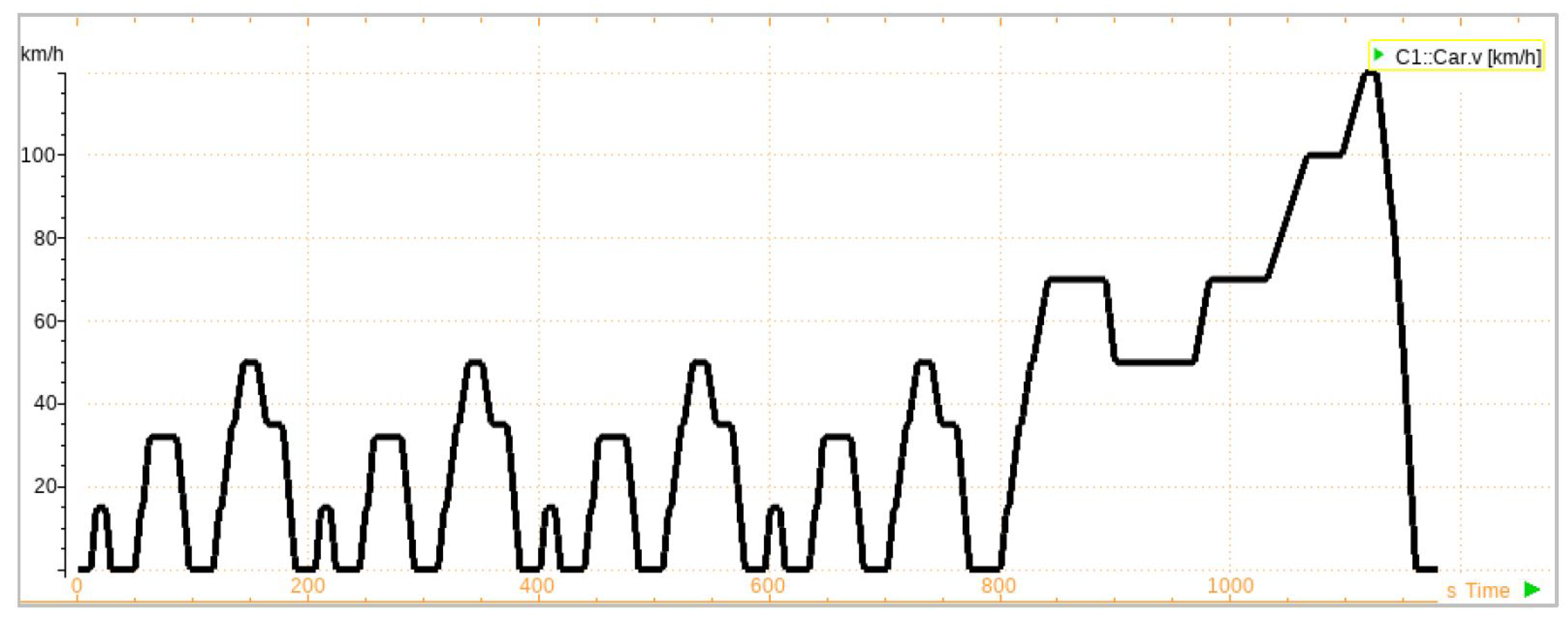
- Target speed: A speed profile is generated during the preparation phase for the entire route. For this purpose, information such as the maximum top speed, braking before curves, acceleration behavior, etc. is used as input. The driver model tries to maintain the specified speed profile throughout the entire simulation process. However, the model can react adaptively to the situation, for example, due to increased traffic volume, and adjust the speed profile [38];
- -
- Vehicle state: The driver model has all the information about the vehicle’s state of movement available at all times. This includes, for example, speed, longitudinal and lateral acceleration, sideslip angle and other relevant data [23].
- -
- Steering wheel torque: Similar to the vehicle state information, this information comes from the vehicle model. For example, if the vehicle’s steering wheel torque is below a certain threshold, it means that the driver model has lost control of the vehicle in the simulation [38].
5. Simulation and Result
5.1. Approach
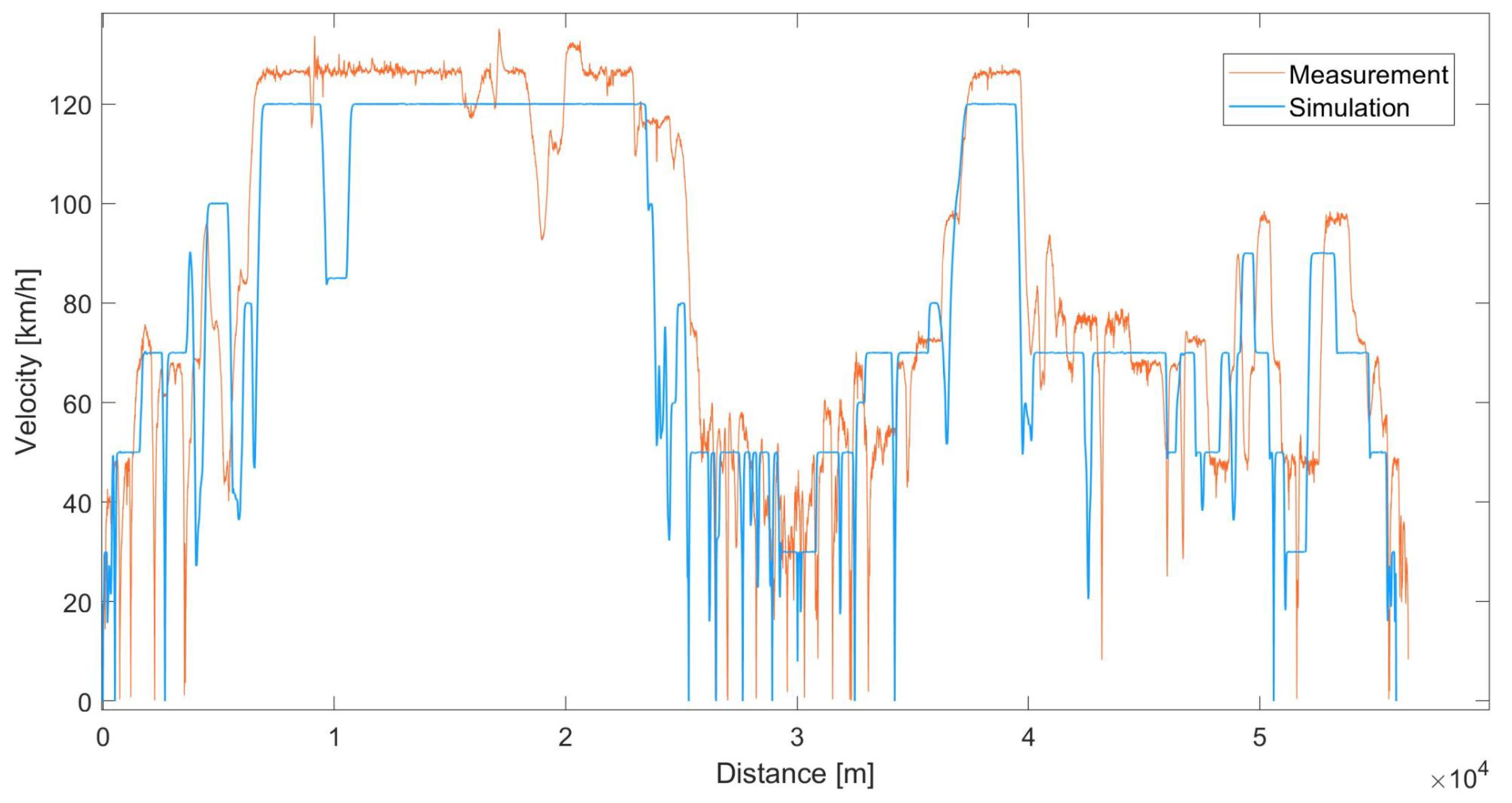
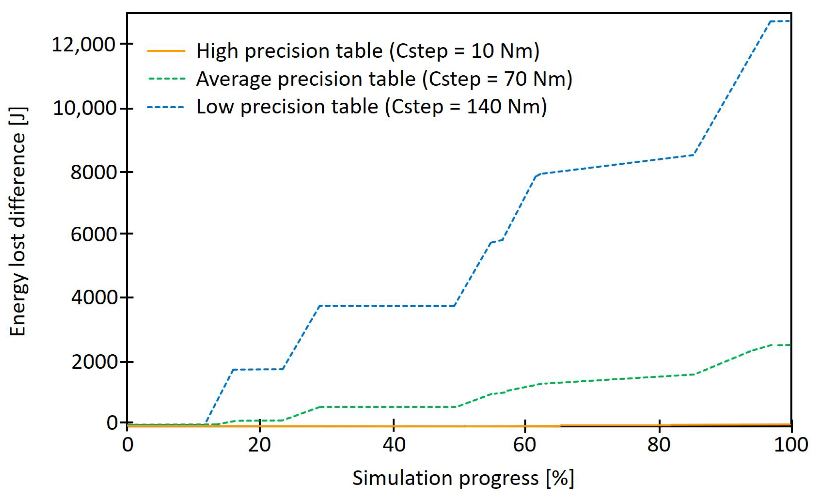
5.2. Results
6. Conclusions and Perspective
Author Contributions
Funding
Acknowledgments
Conflicts of Interest
Abbreviations
| HESS | Hybrid energy storage systems |
| EMS | Energy management system |
| API | Application programming interface |
| NEDC | New European Driving Cycle |
| WLTP | Worldwide harmonized Light vehicles Test Procedure |
| GPS | Global Positioning System |
| SOC | State of charge |
| DC | Direct current |
| NYCC | New York City cycle |
| AU | Artemis urban |
| NY Comp | New York composite cycle |
| TMC | TrafficMessage Channel |
| SRTM | Shuttle Radar Topography Mission |
| MCU | Motor control unit |
| BCU | Battery control unit |
| RMSPE | Root-mean-square percentage error |
| MPE | Maximum percentage error |
| HV | High voltage |
| LV | Low voltage |
References
- Transport and the Green Deal. Available online: https://ec.europa.eu/info/strategy/priorities-2019-024/european-green-deal/transport-and-green-deal_en (accessed on 10 August 2021).
- Grewal, K.S.; Darnell, P.M. Model-based EV range prediction for Electric Hybrid Vehicles. In Proceedings of the IET Hybrid and Electric Vehicles Conference 2013 (HEVC 2013), London, UK, 6–7 November 2013. [Google Scholar]
- Viola, F.; Longo, M.; Zaninelli, D.; Romano, P.; Miceli, R. How is the spread of the Electric Vehicles? In Proceedings of the 2015 IEEE 1st International Forum on Research and Technologies for Society and Industry Leveraging a Better Tomorrow (RTSI), Turin, Italy, 16–18 September 2015. [Google Scholar] [CrossRef]
- Allègre, A.L.; Trigui, R.; Bouscayrol, A. Different energy management strategies of Hybrid Energy Storage System (HESS) using batteries and supercapacitors for vehicular applications. In Proceedings of the 2010 IEEE Vehicle Power and Propulsion Conference, Lille, France, 1–3 September 2010. [Google Scholar]
- Joud, L.; Da Silva, R.; Chrenko, D.; Kéromnès, A.; Le Moyne, L. Smart Energy Management for Series Hybrid Electric Vehicles Based on Driver Habits Recognition and Prediction. Energies 2020, 13, 2954. [Google Scholar] [CrossRef]
- Feng, Y.; Cao, Z.; Shen, W.; Yu, X.; Han, F.; Chen, R.; Wu, J. Intelligent battery management for electric and hybrid electric vehicles: A survey. In Proceedings of the 2016 IEEE International Conference on Industrial Technology (ICIT), Taipei, Taiwan, 14–17 March 2016. INSPEC Accession Number: 16035706. [Google Scholar]
- Miller, J.M. Energy Storage Technology Markets and Application’s: Ultracapacitors in Combination with Lithium-ion. In Proceedings of the 7th International Conference on Power Electronics, Daegu, Korea, 22–26 October 2007. [Google Scholar] [CrossRef]
- Gunasagran, S.K.; Kriesten, R.; Nguyen, T. Implementation of a Model for the Generation of Realistic Energy Flow Based on a Typical Driving Cycle. Bachelor’s Thesis, University of Applied Sciences Karlsruhe—IEEM, Karlsruhe, Germany, 2020. [Google Scholar]
- Fotouhi, A.; Auger, D.J.; Propp, K.; Longo, S. Simulation for prediction of vehicle efficiency, performance, range and lifetime: A review of current techniques and their applicability to current and future testing standards. In Proceedings of the 5th IET Hybrid and Electric Vehicles Conference (HEVC 2014), London, UK, 5–6 November 2014. IET INSPEC Accession Number: 14737982. [Google Scholar]
- Shen, J. Energy Management of a Battery-Ultracapacitor Hybrid Energy Storage System in Electric Vehicles. Ph.D. Thesis, University of Maryland, College Park, MD, USA, 2016. [Google Scholar]
- Shen, J.; Khaligh, A. A Supervisory Energy Management Control Strategy in a Battery/Ultracapacitor Hybrid Energy Storage System. Trans. Transp. Electrif. 2016, 1, 223–231. [Google Scholar] [CrossRef]
- Munoz, P.M.; Correa, G.; Gaudiano, M.E.; Fernández, D. Energy management control design for fuel cell hybrid electric vehicles using neural networks. Int. J. Hydrogen Energy 2017, 42, 28932–28944. [Google Scholar] [CrossRef]
- Hu, J.; Jiang, X.; Jia, M.; Zheng, Y. Energy management strategy for the hybrid energy storage system of pure electric vehicle considering traffic information. Appl. Sci. 2018, 8, 1266. [Google Scholar] [CrossRef]
- Li, J.; Zhou, Q.; He, Y.; Shuai, B.; Li, Z.; Williams, H.; Xu, H. Dual-loop online intelligent programming for driver-oriented predict energy management of plug-in hybrid electric vehicles. Appl. Energy 2019, 253, 113617. [Google Scholar] [CrossRef]
- Fontaras, G.; Ciuffo, B.; Zacharof, N.; Tsiakmakis, S.; Marotta, A.; Pavlovic, J.; Anagnostopoulos, K. The difference between reported and real-world CO2 emissions: How much improvement can be expected by WLTP introduction? Transp. Res. Procedia 2017, 25, 3933–3943. [Google Scholar] [CrossRef]
- Pavlovic, J.; Tansini, A.; Fontaras, G.; Ciuffo, B.; Otura, M.G.; Trentadue, G.; Bertoa, R.S.; Millo, F. The Impact of WLTP on the Official Fuel Consumption and Electric Range of Plug-in Hybrid Electric Vehicles in Europe. In Proceedings of the 2017 SAE 13th International Conference on Engines and Vehicles, Capri, Italy, 12–14 September 2017. SAE Technical Paper JRC107229. [Google Scholar]
- Zhang, Q.; Li, G. A predictive energy management system for hybrid energy storage systems in electric vehicles. Electr. Eng. 2019, 101, 759–770. [Google Scholar] [CrossRef]
- Kruppok, K.; Kriesten, R.; Sax, E. Calculation of route-dependent energy-saving potentials to optimize EV’s range. In 18. Internationales Stuttgarter Symposium 2018; Springer: Stuttgart, Germany, 2018; pp. 1349–1363. [Google Scholar] [CrossRef]
- Zhang, L.; Ye, X.; Xia, X. A Real-Time Energy Management and Speed Controller for an Electric Vehicle Powered by a Hybrid Energy Storage System. IEEE Trans. Ind. Inform. 2020, 16, 6272–6280. [Google Scholar] [CrossRef]
- Kruppok, K. Analyse der Energieeinsparpotenziale zur Bedarfsgerechten Reichweitenerhöhung von Elektrofahrzeugen. Ph.D. Thesis, Karlsruhe Institut für Technologie, Elektrotechnik und Informationstechnik, Karlsruhe, Germany, 2020. [Google Scholar]
- Gutenkunst, C.; Chrenko, D.; Kriesten, R.; Neugebauer, P.; Jaeger, B.; Giereth, T. Route Generating Algorithm Based on OpenSource Data to Predict the Energy Consumption of Different Vehicles. In Proceedings of the 2015 IEEE Vehicle Power and Propulsion Conference (VPPC), Montreal, QC, Canada, 19–22 October 2015. [Google Scholar] [CrossRef]
- IPG Automotive GmbH. Reference Manual Version 8.1.1; CarMaker, IPG Automotive Group: Karlsruhe, Germany, 2019. [Google Scholar]
- IPG Automotive GmbH. User’s Guide Version 8.1.1; CarMaker, IPG Automotive Group: Karlsruhe, Germany, 2019. [Google Scholar]
- Rao, R.; Vrudhula, S.; Rakhmatov, D.N. Battery modeling for energy-aware system design. Computer 2003, 36, 77–87. [Google Scholar] [CrossRef]
- Yao, L.W.; Aziz, J.A.; Kong, P.Y.; Idris, N.R.N. Modeling of lithium-ion battery using MATLAB/simulink. In Proceedings of the IECON 2013, 39th Annual Conference of the IEEE Industrial Electronics Society, Vienna, Austria, 10–13 November 2013; IEEE: Piscataway, NJ, USA, 2013; pp. 1729–1734, ISBN 978-1-4799-0224-8. [Google Scholar]
- Chen, M.; Rincon-Mora, G.A. Accurate electrical battery model capable of predicting runtime and I-V performance. IEEE Trans. Energy Convers. 2006, 21, 504–511, INSPEC Accession Number: 8919488. [Google Scholar] [CrossRef]
- Zhang, H.; Chow, M.-Y. Comprehensive dynamic battery modeling for PHEV applications. In Proceedings of the 2010 IEEE Power and Energy Society General Meeting, [IEEE PES-GM 2010], Minneapolis, MN, USA, 25–29 July 2010; IEEE: Piscataway, NJ, USA, 2010; pp. 1–6, ISBN 978-1-4244-6549-1. [Google Scholar]
- Doerffel, D.; Sharkh, S.A. A critical review of using the Peukert equation for determining the remaining capacity of lead-acid and lithium-ion batteries. J. Power Sources 2006, 155, 395–400. [Google Scholar] [CrossRef]
- Madani, S.; Schaltz, E.; Kaer, K.S. An Electrical Equivalent Circuit Model of a Lithium Titanate Oxide Battery. Batteries 2019, 5, 31. [Google Scholar] [CrossRef]
- Lahyani, A.; Venet, P.; Guermazi, A.; Troudi, A. Battery/Supercapacitors Combination in Uninterruptible Power Supply (UPS). IEEE Trans. Power Electron. 2013, 28, 1509–1522. [Google Scholar] [CrossRef]
- Dougal, R.A.; Gao, L.; Liu, S. Ultracapacitor model with automatic order selection and capacity scaling for dynamic system simulation. J. Power Sources 2004, 126, 250–257. [Google Scholar] [CrossRef]
- Eldeeb, H.H.; Elsayed, A.T.; Lashway, C.R.; Mohammed, O. Hybrid Energy Storage Sizing and Power Splitting Optimization for Plug-In Electric Vehicles. IEEE Trans. Ind. Applicat. 2019, 55, 2252–2262. [Google Scholar] [CrossRef]
- Zubieta, L.; Bonert, R. Characterization of double-layer capacitors for power electronics applications. IEEE Trans. Ind. Applicat. 2000, 36, 199–205. [Google Scholar] [CrossRef]
- Letrouve, T.; Bouscayrol, A.; Lhomme, W.; Dollinger, N.; Calvairac, F.M. Different models of a traction drive for an electric vehicle simulation. In Proceedings of the 2010 IEEE Vehicle Power and Propulsion Conference, Lille, France, 1–3 September 2010. [Google Scholar] [CrossRef]
- Burress, T. Oak Ridge National Laboratory (ORNL), Research Area: Benchmarking Electric Vehicles and Hybrid Electric Vehicles in FY 2016 Annual Progress Report for Electric Drive Technologies Program (2016); U.S. Departement of ENERGY: Washington, DC, USA, July 2017; pp. 196–207.
- Wang, Y.; Wang, L.; Li, M.; Chen, Z. A review of key issues for control and management in battery and ultra-capacitor hybrid energy storage systems. eTransportation 2020, 4, 100064. [Google Scholar] [CrossRef]
- Cao, J.; Emadi, A. A New Battery/UltraCapacitor Hybrid Energy Storage System for Electric, Hybrid, and Plug-In Hybrid Electric Vehicles. IEEE Trans. Power Electron. 2012, 27, 122–132. [Google Scholar] [CrossRef]
- IPG Automotive GmbH. User Manual Version 8.1.1; IPG Driver, IPG Automotive Group: Karlsruhe, Germany, 2019. [Google Scholar]
- Technische Daten BMW i3. Available online: https://www.press.bmwgroup.com/deutschland/article/detail/T0189822DE/technische-daten-bmw-i3-gueltig-ab-03/2014?language=de (accessed on 10 December 2020).
- NEDC Emission Test Cycles. Available online: https://dieselnet.com/standards/cycles/ece_eudc.php (accessed on 16 October 2020).
- Gutenkunst, C. Prädiktive Routenenergieberechnung eines Elektrofahrzeugs. Ph.D. Thesis, University of Applied Sciences Karlsruhe—IEEM, Karlsruhe, Germany, 2020. [Google Scholar]


| OSM | TomTom | HERE | Others | ||
|---|---|---|---|---|---|
| Route | MapQuest, Skobbler, etc. | Directions API | Routing API | Routing API | - |
| Realtime traffic | TMC | Traffic API | Routing API | Traffic API | - |
| Elevation | Open- Elevation API | Elevation API | Search API | Routing API | SRTM |
| Weather | Open- Weather API | - | Advanced- Weather API | Destination- Weather API | SolCast |
| Speed limit | Overpass API | Geocoder API | - | Routing API | - |
| Traffic light | Overpass API | - | - | Advanced Data sets | - |
| Bridge/ Tunnel | Overpass API | - | - | - | - |
| Value | Unit | |
|---|---|---|
| Curb Mass | 1195 | kg |
| Engine Power | 125 | kW |
| Max. Torque | 250 | Nm |
| Max. Velocity | 150 | km/h |
| Length | 3999 | mm |
| Width | 1775 | mm |
| Height | 1579 | mm |
| No. of Electric Motors | 1 | - |
| Capacity of Battery | 61 | Ah |
| Voltage | 360 | V |
| Value | Unit | |
|---|---|---|
| Nominal Voltage | 3.7 | V |
| Nominal Capacity | 61 | Ah |
| Min./Max. Voltage | 2.70/4.10 | V |
| Material Cathode | NCM (Nickel-Cobalt-Manganese) | |
| Value | Unit | |
|---|---|---|
| Nominal Voltage | 2.7 | V |
| Capacitance | 3000 | F |
| ESR | 0.29 | mΩ |
| Usable Specific Power | 5.9 | kW/kg |
| Specific Energy | 6.0 | Wh/kg |
| Stored Energy | 3.04 | Wh |
| Operating Temperature range (min./max.) | −40/65 | °C |
| Storage Temperature range (min./max.) | −40/70 | °C |
| Mass (typical) | 510 | g |
| Unit | Literature | Simulation | Deviation in (%) | |
|---|---|---|---|---|
| Distance | km | 10.93 | 11.01 | 0.73 |
| Duration | s | 1180 | 1180 | 0.00 |
| Range | km | 190 | 188 | −1.05 |
| Energy Demand | kWh/100 km | 11.58 | 11.72 | 1.21 |
Publisher’s Note: MDPI stays neutral with regard to jurisdictional claims in published maps and institutional affiliations. |
© 2022 by the authors. Licensee MDPI, Basel, Switzerland. This article is an open access article distributed under the terms and conditions of the Creative Commons Attribution (CC BY) license (https://creativecommons.org/licenses/by/4.0/).
Share and Cite
Nguyen, T.; Kriesten, R.; Chrenko, D. Concept for Generating Energy Demand in Electric Vehicles with a Model Based Approach. Appl. Sci. 2022, 12, 3968. https://doi.org/10.3390/app12083968
Nguyen T, Kriesten R, Chrenko D. Concept for Generating Energy Demand in Electric Vehicles with a Model Based Approach. Applied Sciences. 2022; 12(8):3968. https://doi.org/10.3390/app12083968
Chicago/Turabian StyleNguyen, Tuyen, Reiner Kriesten, and Daniela Chrenko. 2022. "Concept for Generating Energy Demand in Electric Vehicles with a Model Based Approach" Applied Sciences 12, no. 8: 3968. https://doi.org/10.3390/app12083968
APA StyleNguyen, T., Kriesten, R., & Chrenko, D. (2022). Concept for Generating Energy Demand in Electric Vehicles with a Model Based Approach. Applied Sciences, 12(8), 3968. https://doi.org/10.3390/app12083968