A Novel Hybrid Model for the Prediction and Classification of Rolling Bearing Condition

Abstract

Rotating machinery is a key piece of equipment for tremendous engineering operations. Vibration analysis is a powerful tool for monitoring the condition of rotating machinery. Furthermore, vibration signals have the characteristics of time series. Hence, it is necessary to monitor the condition of vibration signal series to avoid any catastrophic failure. To this end, this paper proposes an effective condition monitoring strategy under a hybrid method framework. First, we add variational mode decomposition (VMD) to preprocess the data points listed in a time order into a subseries, namely intrinsic mode functions (IMFs). Then the framework of the hybrid prediction model, namely the autoregressive moving average (ARMA)-artificial neural network (ANN), is adopted to forecast the IMF series. Next, we select the sensitive modes that contain the prime information of the original signal and that can imply the condition of the machinery. Subsequently, we apply the support vector machine (SVM) classification model to identify the multiple condition patterns based on the multi-domain features extracted from sensitive modes. Finally, the vibration signals from the Case Western Reserve University (CWRU) laboratory are utilized to verify the effectiveness of our proposed method. The comparison results demonstrate advantages in prediction and condition monitoring.

1. Introduction

In practical operation, machinery control technology [1,2,3,4], fault diagnosis and condition monitoring [5,6] have attracted wide research. Vibration analysis is a widely used tool for monitoring the condition of rotating machinery in industrial operation [7,8].

There is abundant information in the time or frequency domain reflecting the characteristics of a machine’s condition; however, some information is not suitable to apply directly. The signal decomposition method can decompose the original signal into a subseries to further comprehensively analyze the signal. Therefore, many researchers have been attracted to the field. A considerable number of techniques have been extensively carried out to fix this issue, such as wavelet decomposition (WT) [9,10]; however, wavelet decomposition aims to find wavelet basis functions, which generates a non-adaptive problem. This is the reason that the wavelet basis function is selected empirically. Different from the WT, empirical mode decomposition (EMD) was presented by Huang et al. [11,12]. Based on the inherent properties of the signal itself, the original signal was empirically decomposed by EMD. Therefore, the data from nonlinear and non-stationary processes can be decomposed by EMD, while a physically meaningful subseries can be obtained based on its adaptive characteristics [13]. Regrettably, the endpoint effect in EMD is still unresolved. Ensemble empirical mode decomposition (EEMD) was introduced by Wu and Huang [14] to alleviate the mode mixing problem occurred in EMD [15], which was a typical noise-assisted data analysis method and also has been widely applied in time-frequency analysis. Furthermore, Wang et al. [16] validated the superiority of EEMD over EMD. Both EMD and EEMD exhibit tremendous computational load and are not suitable for decomposing signals that contain large amounts of data based on their recursive decomposition [17]. In 2013, Dragomiretskiy and Zosso proposed a new algorithm for decomposing signals adaptively called variational mode decomposition (VMD) [18]. VMD is a fully non-recursive method with a more solid mathematical theoretical foundation [19]. Several studies have verified that VMD has better performance over WT, EMD, and EEMD in terms of time-frequency analysis [20,21,22]. Thus, the original signal is decomposed into several sub-series through VMD, which is targeted to enhance the accuracy and convenience of the downstream feature extraction and classification processing.

The vibration signal has the characteristics of a typical time series. It has been found that time series model-based techniques play a pivotal role in monitoring the condition of machinery based on vibration signals [23]. Therefore, an effective time series forecasting model is the key to monitoring the condition of industrial equipment, which can uncover potential statistical patterns through exploring the functional relationships. Furthermore, such patterns can give a valuable early warning. However, it is a challenge to acquire reliable information in practical operations. For time-series analysis and modeling, ARMA is one of the most popular approaches, which has made considerable achievements in various fields in terms of forecasting, such as finance [24,25], engineering [26], and many others [27,28]. In addition, ARMA is more accurate than some other popular machine learning methods in prediction, such as multi-layer perceptron, SVM, and long short-term memory [29,30]. Although ARMA has made great progress in coping with linear analyses based on the assumption that a linear functional relationship exists for current and past values and white noise, its limitations in nonlinear analysis hinder its application. Considerable research on ARMA has demonstrated that its performance is poor in modeling nonlinear real-world problems [31]. For nonlinear time series modeling, ANN is one of the most widely used algorithms [32,33], while the ANN model alone can not give full consideration to both linear and nonlinear patterns simultaneously [31,34]. In summary, any single model can not perform well in every situation. Consequently, considering the merits and drawbacks of ARMA in linear flexibility and ANN for nonlinear time series modeling, their synthetic prediction model, namely, ARMA-ANN, is constructed as a prediction model for subseries in this paper. The motivation for applying the hybrid model is demonstrated as follows [34]. First, instability and uncertainty are common in engineering applications. Second, the time series demonstrates complex characteristics in the real world. Third, each type of individual model rarely perform well compared to the hybrid technique, which combines the advantages of each type of model into an integration. Therefore, using the hybrid technique improves forecasting performance.

Various measurement indicators were considered in vibration signal analysis and fault feature extraction [35,36]. To comprehensively describe the condition information of the original signal, feature extraction plays an important role. Thus, the relevant studies have been widely studied [37,38]. The multi-domain features extracted from the sensitive modes contain the main information of the original signal. The motivation for selecting sensitive IMFs is to avoid the interference of redundant information [39]. SVM is a promising method that can solve the classification problem of small samples [40,41]. Therefore, SVM has been extensively used in mechanical fault classification based on its merits [39,42].

This work proposes an effective hybrid condition monitoring strategy that achieves state-of-the-art performance, which makes predictive maintenance come true [43]. First, we apply VMD to decompose the original signals into several subseries and predict the IMFs by ARMA-ANN. Then, the time-frequency domain (T-F) features are extracted from the sensitive IMFs. Finally, a SVM classifier is used to identify the condition patterns of the rolling bearing based on the T-F features. The performance of our method is verified through experimental signals from the CWRU Laboratory.

Our work mainly provides the following contributions:

First, the key information can be sufficiently captured through VMD decomposing the original signal into subseries to improve the accuracy of feature extraction and classification. Then, the subseries are fed into the hybrid prediction model to provide a reliable trend of the original signal. Next, the excellent accuracy for pattern identification of rolling bearing is acquired based on the comprehensive T-F features. Finally, a sufficient comparable experimental analysis verifies that our method achieved excellent performance while simultaneously relieving time resource problems.

The rest of this study is organized as follows: Section 2 presents the theoretical background. Section 3 introduces the proposed framework in detail. Experimental results and comparisons are presented in Section 4, and conclusions are given in Section 5.

2. Theoretical Foundation

2.1. Variational Model Decomposition

VMD is an adaptive, completely non-recursive variational mode decomposition model. The core idea of VMD is to determine the decomposed K IMFs, their corresponding center frequencies, and bandwidth by iteratively searching the optimal solution of the variational model. The constraint model formula of VMD is as follows:

$$\begin{array}{cc}\hfill & \underset{\left\{u_k\right\},\left\{{\omega }_k\right\}}{min}\sum _{k=1}^K{∥{\partial }_t\left[\left(\delta \left(t\right)+\frac{j}{\pi t}\right)*u_k\left(t\right)\right]e^{-j{\omega }_{k}t}∥}_2^2\hfill \\ \hfill & \begin{array}{cc}\hfill s.t.& \hfill {\displaystyle \sum _{k=1}^K}{u}_k\left(t\right)=x\left(t\right)\end{array},\hfill \end{array}$$

(1)

where $x\left(t\right)$ is the original signal and $\left\{u_k\right\}:=\left\{u_1,u_2,\cdots u_K\right\}$ and $\left\{{\omega }_k\right\}:=\left\{{\omega }_1,{\omega }_2,\cdots {\omega }_K\right\}$ represent the set of all modes and the corresponding center frequencies, respectively. $\delta \left(t\right)$ is the Dirac distribution, ${\partial }_t$ is the partial with respect to t, and K is the number of modes to be decomposed (positive integer). To solve the optimal solution of the constraint model, the augmented Lagrange function method is introduced to transform the constraint problem into an unconstrained problem, and its formula is as follows:

$$\begin{array}{c}\hfill \mathcal{L}\left(\left\{u_k\right\},\left\{{\omega }_k\right\},\lambda \right):=\alpha \sum _{k=1}^K{∥{\partial }_t\left[\left(\delta \left(t\right)+\frac{j}{\pi t}\right)*u_k\left(t\right)\right]e^{-j{\omega }_{k}t}∥}_2^2\\ \hfill +{∥x\left(t\right)-\sum _{k=1}^K{u}_k\left(t\right)∥}_2^2+〈\lambda \left(t\right),x\left(t\right)-\sum _{k=1}^K{u}_k\left(t\right)〉,\end{array}$$

(2)

where $\alpha$ is the quadratic penalty term and $\lambda \left(t\right)$ is the Lagrange multipliers. The alternate direction method of multipliers is adopted to settle the optimal $u_k$, ${\omega }_k$ and $\lambda \left(t\right)$, which can be written as:

$${\widehat{u}}_k^{n+1}\leftarrow \frac{{\displaystyle \widehat{f}\left(\omega \right)-\sum _{i<k}{\widehat{u}}_i^{n+1}\left(\omega \right)-\sum _{i>k}{\widehat{u}}_i^n\left(\omega \right)+\frac{{\widehat{\lambda }}^n\left(\omega \right)}{2}}}{1+2\alpha {(\omega -{\omega }_k^n)}^2},$$

(3)

$${\omega }_k^{n+1}\leftarrow \frac{{\int }_0^{\infty }\omega {\left|{\widehat{u}}_k^{n+1}\left(\omega \right)\right|}^{2}d\omega }{{\int }_0^{\infty }{\left|{\widehat{u}}_k^{n+1}\left(\omega \right)\right|}^{2}d\omega },$$

(4)

$${\widehat{\lambda }}^{n+1}\left(\omega \right)\leftarrow {\widehat{\lambda }}^n\left(\omega \right)+\tau \left(\widehat{x}\left(\omega \right)-\sum _k{\widehat{u}}_k^{n+1}\left(\omega \right)\right).$$

where $\widehat{u}\left(\omega \right)$, $\widehat{\omega }$ and $\widehat{\lambda }\left(\omega \right)$ denote the Fourier transforms of each variable, and n is the number of iteration. Ref. [18] provided more details on the VMD algorithm.

2.2. Prediction Model

Two popular forecasting models, ARMA and ANN, will be introduced in this section, which also will be used to predict the IMFs in our research.

2.2.1. Autoregressive Moving Average Model

The ARMA model is designed for the variables for which past observations imply a linear function with the future value. ARMA is first used to predict the IMF series. Because the response of IMF $Y_{lt}$ at t is related to the response of its previous time $Y_{t-1},Y_{t-2},\dots ,Y_{t-p}$, it is also affected by q random errors, namely ${\epsilon }_{t-1},{\epsilon }_{t-2},\dots ,{\epsilon }_{t-q}$. For the ARMA $\left(p,q\right)$ model,

$${\widehat{Y}}_{lt}={\beta }_1{Y}_{t-1}+{\beta }_2{Y}_{t-2}+\dots +{\beta }_p{Y}_{t-p}+{\epsilon }_t-{\theta }_1{\epsilon }_{t-1}-{\theta }_2{\epsilon }_{t-2}+\dots +{\theta }_q{\epsilon }_{t-q},$$

(5)

provides high accuracy prediction, where ${\beta }_p\left(p=1,2,\dots \right)$ and ${\theta }_q\left(q=1,2,\dots \right)$ are the auto-regression (AR) and moving average (MA) coefficients, respectively. p, q are the orders of the ARMA model, which are identified based on Akaike’s information criterion and Bayesian information criterion in this paper. When $q=0$, the model is reduced to an AR $\left(p\right)$ model. If $p=0$, the model is reduced to a MA $\left(q\right)$ model. Note that $E\left({\epsilon }_t\right)=0$, $Var\left({\epsilon }_t\right)={\sigma }_{\epsilon }^2$.

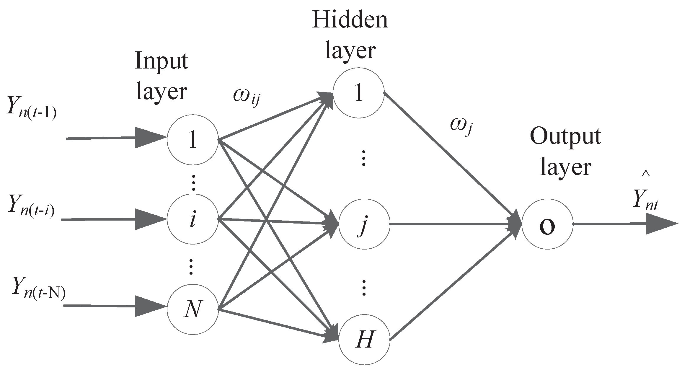
2.2.2. Artificial Neural Network Model

ANN is a tool which can detect all possible interactions between the input and output from the provided training data. It also provides a flexible architecture for nonlinear modeling in fault detection, diagnosis [44], and prediction [45]. The framework of ANN depends on the characteristics of the data. Thus, the number layers and neurons are configured based on the essence of the input data. The widely used three-layer ANN model presented in Figure 1 is applied to model time series data, in which the neurons are acyclically linked.

The nonlinear function f of $Y_{nt}$ sequence from $Y_{n\left(t-1\right)}$ to $Y_{n\left(t-N\right)}$ is expressed as follows:

$${\widehat{Y}}_{nt}={\omega }_0+\sum _{j=1}^H{\omega }_{j}f\left({\omega }_{0j}+\sum _{i=1}^N{\omega }_{ij}{Y}_{n\left(t-i\right)}\right)+e_t,$$

(6)

where ${\widehat{Y}}_{nt}$ is the prediction result at any given time t, ${\omega }_{ij}$ and H denote the hidden layer neuron weights and number, respectively. The corresponding input layers are ${\omega }_j$ and N. f represents a “sigmoid” function in this research, while $e_t$ is a noise or error term. Additionally, to avoid the local minimum and overfitting, k-fold cross validation is applied to train the ANN. Finally, we evaluate the test data with the trained ANN [46].

2.2.3. Hybrid Prediction Model

We take the original time series data $Y_t$ as consisting of two components, the linear components $Y_{lt}$ and the nonlinear components $Y_{nt}$. The residual data $r_t=Y_t-Y_{lt}$ are considered as the distinction between the linear component and original data. Thus, the hybrid model is constructed as:

$$\begin{array}{c}\hfill \begin{array}{c}\hfill \left\{\begin{array}{cc}{\displaystyle }\hfill & {\widehat{Y}}_{lt}={\beta }_1{Y}_{t-1}+{\beta }_2{Y}_{t-2}+\dots +{\beta }_p{Y}_{t-p}+{\epsilon }_t-{\theta }_1{\epsilon }_{t-1}-{\theta }_2{\epsilon }_{t-2}+\dots +{\theta }_q{\epsilon }_{t-q}\hfill \\ {\displaystyle }\hfill & {\widehat{Y}}_t={\widehat{Y}}_{lt}+{\widehat{Y}}_{nt}\hfill \\ {\displaystyle }\hfill & Y_{nt}=Y_t-{\widehat{Y}}_{lt}\hfill \\ {\displaystyle }\hfill & {\displaystyle {\widehat{Y}}_{nt}={\omega }_0+\sum _{j=1}^H{\omega }_{j}f\left({\displaystyle {\omega }_{0j}+\sum _{i=1}^N{\omega }_{ij}{Y}_{n\left(t-i\right)}}\right)+e_t}\hfill \end{array}\right.,\end{array}\end{array}$$

(7)

where ${\widehat{Y}}_t$ is the final prediction result, ${\widehat{Y}}_{lt}$ is the ARMA prediction result, $Y_{nt}$ is the residual of the ARMA model, and ${\widehat{Y}}_{nt}$ is the prediction result of the ANN model.

2.3. Feature Extraction

Both time-domain and frequency-domain indicators are affected by the equipment’s operating condition [19].

Table 1. The expression of feature parameters.

Time-Domain Parameter	Feature Expression	Frequency-Domain Parameter	Feature Expression
F1	$|max\left(x_i\right)-min\left(x_i\right)|$	F6	$\frac{{\sum }_{i=1}^N{f}_{i}G\left(f_i\right)}{{\sum }_{i=1}^{N}G\left(f_i\right)}$
F2	$\frac{max\left(x_i\right)}{\frac{1}{N}{\sum }_{i=1}^N\left|x_i\right|}$	F7	$\frac{{\sum }_{i=1}^N{f}_{i}G\left(f_i\right)}{{\sum }_{i=1}^N\left(f_i\right)}$
F3	$\frac{max\left(x_i\right)}{{\left(\frac{1}{N}{\sum }_{i=1}^N\sqrt{|x_i|}\right)}^2}$	F8	$\frac{{\sum }_{i=1}^N{\left(f_i-F6\right)}^{2}G\left(f_i\right)}{{\sum }_{i=1}^{N}G\left(f_i\right)}$
F4	$\frac{1}{N}{\sum }_{i=1}^N\frac{{\left(x_i-\mu \right)}^3}{{\sigma }^3}$	F9	$\frac{1}{N}{\sum }_{i=1}^{N}G\left(f_i\right)$
F5	$\frac{1}{N}{\sum }_{i=1}^N\frac{{\left(x_i-\mu \right)}^4}{{\sigma }^4}$	F10	$\frac{{\sum }_{i=1}^N{f}_i^{2}G\left(f_i\right)}{\sqrt{{\sum }_{i=1}^{N}G\left(f_i\right)*{\sum }_{i=1}^N{f}_i^{4}G\left(f_i\right)}}$

presents the features extracted from the sensitive IMFs, which are the subseries that contain 90% of the energy of the original signal. The energy of each IMF can refer to the Ref. [47].

2.4. Support Vector Machine

SVM is one of the most celebrated and popular classification algorithms in the field of multi-classification [39,40,48]. The prime purpose of SVM is to maximize the margin of between-class, meanwhile narrowing the distance between the hyperplane focuses. The training set of SVM is denoted by

$$S=\left\{{\left(x_i,y_i\right)}_{i=1}^n|x_i\in {\mathcal{R}}^N,y_i\in \left\{-1,1\right\},i=1,2,\dots ,n\right\},$$

where $x_i$ and $y_i$ are the sample data and category, respectively. The hyperplane can separate the data correctly with the maximum interval. The solution of the optimal separating plane is described as:

$$\begin{array}{c}\hfill \begin{array}{c}\hfill \left\{\begin{array}{cc}\hfill & min\frac{1}{2}{\parallel \omega \parallel }^2\hfill \\ \hfill & s.t.y_i\left(\mathit{\omega }{x}_i+\mathit{b}\right)\ge 1\hfill \end{array}\right.,\end{array}\end{array}$$

(8)

where $\mathit{b}$ is the bias vector, $\mathit{\omega }$ denotes the weight vector, and ${\xi }_i\ge 0\left(i=1,2,\dots ,n\right)$ represents a relaxing factor, which ensures the accuracy of classification. We rewrite the problem (8) as the following minimization problem:

$$\begin{array}{c}\hfill \begin{array}{c}\hfill \left\{\begin{array}{cc}\hfill & {\displaystyle min\frac{1}{2}{\parallel \omega \parallel }^2+\lambda \sum _{i=1}^n{\xi }_i\left(\xi \ge 0\right)}\hfill \\ \hfill & s.t.\left\{\begin{array}{c}{y}_i\left(\mathit{\omega }{x}_i+\mathit{b}\right)\ge 1-{\xi }_i\left(i=1,2,\dots ,n\right)\hfill \\ \lambda \ge 0\hfill \end{array}\right.\hfill \end{array}\right.,\end{array}\end{array}$$

(9)

where $\lambda$ is the penalty factor, which is used to relieve the SVM classifier dilemma between accuracy and complexity. The classical hinge loss function is applied in this research. Thus, the dual optimization problem of SVM is described as:

$$\begin{array}{c}\hfill \begin{array}{c}\hfill \left\{\begin{array}{cc}{\displaystyle }\hfill & {\displaystyle maxL\left({\alpha }_i\right)=\sum _{i=1}^n{\alpha }_i-\frac{1}{2}\sum _{i=1}^n\sum _{j=1}^n{\alpha }_i{\alpha }_j{y}_i{y}_{j}K\left(x_i,x_j\right)}\hfill \\ \hfill & s.t.\left\{\begin{array}{c}{\displaystyle \sum _{i=1}^n{\alpha }_i{y}_i=0}\hfill \\ 0\le {\alpha }_i\le \lambda ,i=1,2,\dots ,n\hfill \end{array}\right.\hfill \end{array}\right.,\end{array}\end{array}$$

(10)

where $K\left(x_i,x_j\right)$ denotes a kernel function, $K\left(x_i,x_j\right)=〈{\Phi }^{⊺}\left(x_i\right)·\Phi \left(x_j\right)〉$, and · is the inner product operation. The SVM classifier with a radial basis function (RBF) kernel, $K\left(x_i,x_j\right)=ex{p}^{-\gamma \parallel \left(x_i-x_j\right){\parallel }^2},\gamma >0$ is applied in this work, where $\gamma$ is a hyper-parameter that affects the merits of the SVM. Thus, the classification is described as:

$$\begin{array}{c}\hfill S\left(x\right)=sign\left(\sum _{i=1}^n{\alpha }_i{y}_i〈{\Phi }^{⊺}\left(x_i\right)·\Phi \left(x_j\right)〉\right)+b.\end{array}$$

(11)

3. Proposed Architecture

An architecture for the condition monitoring of the rolling bearing is shown in Figure 2, which is mainly divided into four submodules (VMD decomposition, ARMA-ANN prediction, T-F features extraction and SVM classification).

The specific details are as follows.

(1)

The VMD algorithm decomposes the multi-component vibration signal of rolling bearing into several IMFs. The descriptions of the VMD algorithm are presented in Section 2.1;

(2)

Based on the established ARMA-ANN prediction model, the prediction of each IMF is conducted, and the sensitive IMFs are selected;

(3)

The multi-domain features set, i.e., T-F features set including time domain and frequency domain, are extracted as characteristic parameters from the sensitive IMFs. The specific features are presented in Section 2.3;

(4)

The classification of the condition is performed by a SVM classifier based on T-F features.

4. Experimental Analysis

4.1. Data Description

In this section, the motor bearing data set from the CWRU laboratory is utilized to demonstrate the advantages of our proposed method. More details on the experiment are referenced in [19,49].

4.2. Experimental Results and Analysis

In this paper, four classes of bearing operating conditions data sets, including normal (NS), inner race fault (IF), outer race fault (OF), and ball fault (BF) were applied, respectively. Each piece of the data set consisted of 12,000 points. The working speed, fault size, load and sampling frequency were set to 1730 r/min, 0.007 in, 3 HP, 12 kHz, respectively.

4.2.1. Decomposing the Vibration Signal Using VMD

According to the steps in Section 3, a group of IF data as an example was analyzed.

Table 2. Parameter settings for VMD.

Algorithm	Parameter	Setting
VMD	K	6
	$\alpha$	2891
	DC	0
	tau	0
	init	1
	tol	${10}^{-7}$

shows the VMD relevant parameters according to [19]. The time-waveform of the original signal and the modes obtained by VMD are presented in the left of Figure 3, and the corresponding frequency spectrums are presented in the right of this figure.

4.2.2. Prediction Based on Hybrid Prediction Model

Based on the aforementioned VMD, the original signal was decomposed into several IMF time series, using the hybrid prediction model to obtain the trend of subseries. First, the obtained six IMF series by VMD were subjected to ARMA. We used the AR model of order 12 (AR(12)) and MA model of order 16 (MA(16)) for IMF1. Then the three-layered $1\times 4\times 2$ ANN architecture was used for the residuals. Figure 4, Figure 5 and Figure 6 present the expectations and predictions of IF IMF1 series for ARMA, ANN and ARMA-ANN, respectively. The predictions of the IMF1 for NS, BF, OF, using ARMA-ANN are presented in Figure 7, Figure 8 and Figure 9, respectively.

To further quantify the performance of the prediction models, the comparison of quantitative criteria is shown in

Table 3. Comparison of performance criteria of three models for all dataset series.

Condition	Model	RMSE	MAPE	MAE
IF	ARMA	1.0279 × ${10}^{-1}$	1.1276 × ${10}^0$	8.2175 × ${10}^{-2}$
	ANN	9.6119 × ${10}^{-2}$	2.9847 × ${10}^0$	7.5156 × ${10}^{-2}$
	ARMA-ANN	3.6904 × ${10}^{-4}$	2.2367 × ${10}^{-2}$	2.6025 × ${10}^{-4}$
NS	ARMA	1.4100 × ${10}^{-2}$	1.8500 × ${10}^0$	1.1707 × ${10}^{-2}$
	ANN	1.1744 × ${10}^{-2}$	1.8433 × ${10}^0$	9.4530 × ${10}^{-3}$
	ARMA-ANN	4.6082 × ${10}^{-4}$	3.0578 × ${10}^{-2}$	2.9941 × ${10}^{-4}$
BF	ARMA	4.2184 × ${10}^{-2}$	1.3759 × ${10}^0$	3.4340 × ${10}^{-2}$
	ANN	3.9973 × ${10}^{-2}$	4.0775 × ${10}^0$	3.2100 × ${10}^{-2}$
	ARMA-ANN	8.1888 × ${10}^{-4}$	4.3402 × ${10}^{-2}$	2.6100 × ${10}^{-4}$
OF	ARMA	1.2997 × ${10}^{-1}$	1.0736 × ${10}^0$	1.0533 × ${10}^{-1}$
	ANN	1.2400 × ${10}^{-1}$	2.1900 × ${10}^0$	9.9000 × ${10}^{-2}$
	ARMA-ANN	2.4100 × ${10}^{-3}$	2.9969 × ${10}^{-2}$	1.5100 × ${10}^{-3}$

, including the root-mean-square error (RMSE): $\sqrt{\frac{1}{n}{\sum }_{t=1}^n{e}_t^2}$, the mean average percentage error (MAPE): $\frac{100\%}{n}{\sum }_{t=1}^n\left|\frac{e_t}{Y_t}\right|$, and the mean absolute error (MAE): $\frac{1}{n}{\sum }_{t=1}^n|e_t|$, which are used to quantify the prediction accuracy, where $e_t$ denotes the error between expectation and the prediction.

We further compared the prediction of subseries with the original data series. The prediction of the IF original data series for the ARMA-ANN obtained by VMD is shown in Figure 10.

The quantitative evaluation criteria shown in

Table 4. Comparison of performance criteria of ARMA-ANN model for the original series and subseries.

Condition	Series	RMSE	MAPE	MAE
IF	Original	5.2744 × ${10}^{-3}$	3.0023 × ${10}^{-1}$	4.1815 × ${10}^{-3}$
	Subseries	3.6904 × ${10}^{-4}$	2.2367 × ${10}^{-2}$	2.6025 × ${10}^{-4}$
NS	Original	5.3683 × ${10}^{-3}$	3.1319 × ${10}^{-1}$	4.2680 × ${10}^{-3}$
	Subseries	4.6082 × ${10}^{-4}$	3.0578 × ${10}^{-2}$	2.9941 × ${10}^{-4}$
BF	Original	5.2354 × ${10}^{-3}$	3.0846 × ${10}^{-1}$	4.1308 × ${10}^{-3}$
	Subseries	8.1888 × ${10}^{-4}$	4.3402 × ${10}^{-2}$	2.6100 × ${10}^{-4}$
OF	Original	5.1080 × ${10}^{-3}$	3.0283 × ${10}^{-1}$	4.0719 × ${10}^{-3}$
	Subseries	2.4100 × ${10}^{-3}$	2.9969 × ${10}^{-2}$	1.5100 × ${10}^{-3}$

demonstrate that the prediction of subseries obtained by VMD achieves better performance than the original data series.

This result motivated us to make original data series into subseries to improve the accuracy of results. Furthermore, our hybrid prediction method with VMD could provide a superior scheme for machinery condition monitoring.

4.2.3. Feature Extraction

Next, the features were extracted from the sensitive IMFs. The power spectral density (PSD) distribution of the original signal are shown in Figure 11, which demonstrates that the sensitive modes are the 2nd IMF to the 6th IMF. However, the 1st is obviously redundant for the downstream feature extraction and classification processing. Then, we extracted the T-F features from the 2nd IMF to the 6th IMF to form a new feature set and also normalized the set.

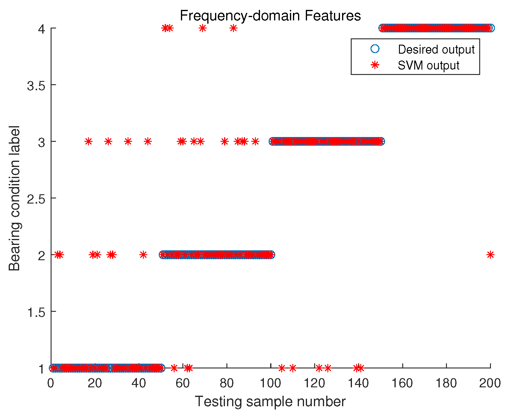
4.2.4. Classification Based on SVM

In this subsection, the condition patterns are identified using SVM based on the normalized feature set. The performance of classification highly depended on the features set. Consequently, the time-domain features and the frequency-domain features were combined to construct the input data vectors. Then, a normalized 10-dimension input vector was fed into SVM to train for the downstream classification processing. Figure 12, Figure 13 and Figure 14 show the recognition results based on the features of different domains.

The quantitative classification performance of the SVM is compared in

Table 5. Comparison of the classification results by using different features.

Domain	Classification Accuracy				Average Accuracy
	IF	BF	OF	Normal
Time domain	94%	86%	98%	96%	93.5%
Frequency domain	78%	68%	88%	98%	83%
Time-frequency domain	98%	88%	98%	96%	95%

, which shows the classification results of the condition patterns using the features of different domains.

The classification accuracy of individual time-domain features or individual frequency-domain features is poor as compared to the time-frequency domain features. These results suggest that either time domain or frequency domain alone cannot fully capture the condition patterns. To tackle this problem, it would be effective to make use of each of the domain features to comprehensively describe all patterns.

In terms of the computational complexity [50,51] and the number of sample points $N_d$ with d dimensions to be trained, the computational complexity of the training phase required could be O$\left(N_d^{2}d\right)$. In the test phase, the computational complexity required O$\left(MN\right)$ operations, where M and N are the kernel operations and support vectors, respectively. The computational complexity of SVM in this example, specifically the 400 points with 50 dimension T-F features to be trained, required the computational complexity to be O$\left({400}^2\times 50\right)$. The RBF kernel was evaluated for 200 operations requiring 307 support vectors. Therefore, the computational complexity required O$\left(200\times 307\right)$ for the test phase.

4.2.5. Discussion

Considerable achievements have been made in time series forecasting [52] and classification [53] for the deep learning-based methods; however, these methods highly depend on the input scale level. Meanwhile, it is worthy to notice that the deep learning-based methods show accuracy associated with the scale level, and the more scales contribute, the more accurate and stable the performance becomes. Therefore, the solution to acquire high performance is costly in terms of time to train and test. This fact indicates that the augmentation of computation becomes the problem caused by its scale level. Moreover, most of the deep learning-based methods cannot deal with a small sample of data; in other words, accuracy and stability cannot be guaranteed in this case.

This research uses 12,000 sample points to verify the performance of the prediction and classification. The biggest challenge is that the data used for training are much less. The reason for this is that our proposed method is conducted to monitor the rolling bear operating condition. Moreover, our strategy for condition monitoring is also effective while simultaneously relieving time resource problems. A detailed description of the comparative method’s parameters is given as follows. The LSTM [52] is utilized to forecast the future trend of the subseries, and “Sigmoid” and “Adam” are utilized as the activation function and optimizer, respectively. The network is updated by minimizing the mean square error for $e_t$ with a gradient descent algorithm. The configurations of the three one-dimensional CNN [53] for classifying layers are: Conv1D $\left(16,64,16\right)$, Conv1D $\left(32,3,1\right)$, Conv1D $\left(64,3,1\right)$. After the convolution operation, the Batch Normalization is carried out. “Relu” is applied as an activation function. Then, the convolution kernel $\left(2\times 1\right)$ is employed in the maximum pooling operation. To more clearly illustrate the advantages of our proposed method on time series forecasting using the same small sample data set, a comparison of quantitative criteria for prediction results is presented in

Table 6. Comparison of performance criteria of prediction results for ARMA-ANN and LSTM.

Operating Condition	Method	RMSE	MAPE	MAE
Inner Race	LSTM	5.5412 × ${10}^{-2}$	7.0271 × ${10}^{-1}$	4.1816 × ${10}^{-2}$
	ARMA-ANN	5.2744 × ${10}^{-3}$	3.0023 × ${10}^{-1}$	4.1815 × ${10}^{-3}$
Normal	LSTM	1.2815 × ${10}^{-2}$	4.5444 × ${10}^{-1}$	9.6361 × ${10}^{-3}$
	ARMA-ANN	5.3683 × ${10}^{-3}$	3.1319 × ${10}^{-1}$	4.2680 × ${10}^{-3}$
Ball	LSTM	2.8762 × ${10}^{-2}$	4.0346 × ${10}^{-1}$	2.1655 × ${10}^{-2}$
	ARMA-ANN	5.2354 × ${10}^{-3}$	3.0846 × ${10}^{-1}$	4.1308 × ${10}^{-3}$
Outer Race	LSTM	1.0495 × ${10}^{-1}$	1.3158 × ${10}^0$	7.7409 × ${10}^{-2}$
	ARMA-ANN	5.1080 × ${10}^{-3}$	3.0283 × ${10}^{-1}$	4.0719 × ${10}^{-3}$

. Our proposed method outperforms the CNN-based method in classification, whose averaged accuracy is higher than $91.88\%$. Therefore, both the performance of prediction and classification confirm the advantages of our proposed method.

5. Conclusions

In this paper, an effective condition monitoring scheme is designed for rolling bearings. First, the original signal can be sufficiently described by IMFs obtained by VMD. Next, each IMF is forecasted through the hybrid prediction model ARMA-ANN. Moreover, the sensitive IMFs, which contain over 90% of the energy of the original signal, are selected to provide downstream feature extraction and classification processing. Then, the T-F features, which can represent the comprehensive condition characteristics of the rolling bearing, are extracted and normalized. Finally, the normalized T-F features are fed into the SVM classifier to identify the operating patterns of the rolling bearing. The performance of the proposed condition monitoring method is verified by the motor-bearing data set of the CWRU laboratory.

Note that the scheme of the original signal first decomposed by VMD into a subseries provides the sufficiency and convenience of analyzing the operating condition. Secondly, the hybrid prediction model enhances the accuracy of prediction. Thirdly, the condition patterns are identified accurately using a SVM classifier based on the T-F features. Additionally, the proposed method balances the performance and time resources equally well. Thus, it can be concluded that our proposed method under the hybrid framework has some potential value for monitoring machinery condition.

References

1. Shen, X.; Wu, Y.; Shen, T. Logical control scheme with real-time statistical learning for residual gas fraction in IC engines. Sci. China Inf. Sci. 2018, 61, 010203. [Google Scholar] [CrossRef]
2. Wu, Y.; Shen, T. Policy iteration approach to control residual gas fraction in IC engines under the framework of stochastic logical dynamics. IEEE Trans. Control. Syst. Technol. 2016, 25, 1100–1107. [Google Scholar] [CrossRef]
3. Zhang, Y.; Shen, X.; Wu, Y.; Shen, T. On-board knock probability map learning–based spark advance control for combustion engines. Int. J. Engine Res. 2019, 20, 1073–1088. [Google Scholar] [CrossRef]
4. Wu, Y.; Guo, Y.; Toyoda, M. Policy iteration approach to the infinite horizon average optimal control of probabilistic Boolean networks. IEEE Trans. Neural Netw. Learn. Syst. 2020, 32, 2910–2924. [Google Scholar] [CrossRef] [PubMed]
5. Brito, L.C.; Susto, G.A.; Brito, J.N.; Duarte, M.A. An explainable artificial intelligence approach for unsupervised fault detection and diagnosis in rotating machinery. Mech. Syst. Signal Process. 2022, 163, 108105. [Google Scholar] [CrossRef]
6. Liu, R.; Yang, B.; Zio, E.; Chen, X. Artificial intelligence for fault diagnosis of rotating machinery: A review. Mech. Syst. Signal Process. 2018, 108, 33–47. [Google Scholar] [CrossRef]
7. Randall, R.B. Vibration-Based Condition Monitoring: Industrial, Automotive and Aerospace Applications; John Wiley & Sons: Hoboken, NJ, USA, 2021. [Google Scholar]
8. Vishwakarma, M.; Purohit, R.; Harshlata, V.; Rajput, P. Vibration analysis & condition monitoring for rotating machines: A review. Mater. Today Proc. 2017, 4, 2659–2664. [Google Scholar]
9. Wang, D.; Miao, Q.; Fan, X.; Huang, H.Z. Rolling element bearing fault detection using an improved combination of Hilbert and wavelet transforms. J. Mech. Sci. Technol. 2009, 23, 3292–3301. [Google Scholar] [CrossRef]
10. Li, Z.; Feng, Z.; Chu, F. A load identification method based on wavelet multi-resolution analysis. J. Sound Vib. 2014, 333, 381–391. [Google Scholar] [CrossRef]
11. Huang, N.E.; Shen, Z.; Long, S.R.; Wu, M.C.; Shih, H.H.; Zheng, Q.; Yen, N.C.; Tung, C.C.; Liu, H.H. The empirical mode decomposition and the Hilbert spectrum for nonlinear and non-stationary time series analysis. Proc. R. Soc. Lond. Ser. A Math. Phys. Eng. Sci. 1998, 454, 903–995. [Google Scholar] [CrossRef]
12. Huang, N.E.; Wu, Z. A review on Hilbert-Huang transform: Method and its applications to geophysical studies. Rev. Geophys. 2008, 46. [Google Scholar] [CrossRef] [Green Version]
13. Huang, N.E. Introduction to the Hilbert–Huang transform and its related mathematical problems. In Hilbert–Huang Transform and Its Applications; World Scientific: Singapore, 2014; pp. 1–26. [Google Scholar]
14. Wu, Z.; Huang, N.E. Ensemble empirical mode decomposition: A noise-assisted data analysis method. Adv. Adapt. Data Anal. 2009, 1, 1–41. [Google Scholar] [CrossRef]
15. Lei, Y.; He, Z.; Zi, Y. Application of the EEMD method to rotor fault diagnosis of rotating machinery. Mech. Syst. Signal Process. 2009, 23, 1327–1338. [Google Scholar] [CrossRef]
16. Wang, T.; Zhang, M.; Yu, Q.; Zhang, H. Comparing the applications of EMD and EEMD on time–frequency analysis of seismic signal. J. Appl. Geophys. 2012, 83, 29–34. [Google Scholar] [CrossRef]
17. Zhang, X.; Sun, T.; Wang, Y.; Wang, K.; Shen, Y. A parameter optimized variational mode decomposition method for rail crack detection based on acoustic emission technique. Nondestruct. Test. Eval. 2021, 36, 411–439. [Google Scholar] [CrossRef]
18. Dragomiretskiy, K.; Zosso, D. Variational mode decomposition. IEEE Trans. Signal Process. 2013, 62, 531–544. [Google Scholar] [CrossRef]
19. Lei, Z.; Wen, G.; Dong, S.; Huang, X.; Zhou, H.; Zhang, Z.; Chen, X. An intelligent fault diagnosis method based on domain adaptation and its application for bearings under polytropic working conditions. IEEE Trans. Instrum. Meas. 2020, 70, 3505914. [Google Scholar] [CrossRef]
20. Wang, Y.; Markert, R.; Xiang, J.; Zheng, W. Research on variational mode decomposition and its application in detecting rub-impact fault of the rotor system. Mech. Syst. Signal Process. 2015, 60, 243–251. [Google Scholar] [CrossRef]
21. Wang, X.B.; Yang, Z.X.; Yan, X.A. Novel particle swarm optimization-based variational mode decomposition method for the fault diagnosis of complex rotating machinery. IEEE/ASME Trans. Mechatron. 2017, 23, 68–79. [Google Scholar] [CrossRef]
22. Lian, J.; Liu, Z.; Wang, H.; Dong, X. Adaptive variational mode decomposition method for signal processing based on mode characteristic. Mech. Syst. Signal Process. 2018, 107, 53–77. [Google Scholar] [CrossRef]
23. Chen, Y.; Liang, X.; Zuo, M.J. Sparse time series modeling of the baseline vibration from a gearbox under time-varying speed condition. Mech. Syst. Signal Process. 2019, 134, 106342. [Google Scholar] [CrossRef]
24. Doroudyan, M.H.; Niaki, S.T.A. Pattern recognition in financial surveillance with the ARMA-GARCH time series model using support vector machine. Expert Syst. Appl. 2021, 182, 115334. [Google Scholar] [CrossRef]
25. Zaw, T.; Kyaw, S.S.; Oo, A.N. ARMA Model for Revenue Prediction. In Proceedings of the 11th International Conference on Advances in Information Technology, Bangkok, Thailand, 1–3 July 2020; pp. 1–6. [Google Scholar]
26. Zhang, Y.; Zhao, Y.; Kong, C.; Chen, B. A new prediction method based on VMD-PRBF-ARMA-E model considering wind speed characteristic. Energy Convers. Manag. 2020, 203, 112254. [Google Scholar] [CrossRef]
27. Bang, S.; Bishnoi, R.; Chauhan, A.S.; Dixit, A.K.; Chawla, I. Fuzzy Logic based Crop Yield Prediction using Temperature and Rainfall parameters predicted through ARMA, SARIMA, and ARMAX models. In Proceedings of the 2019 Twelfth International Conference on Contemporary Computing (IC3), Noida, India, 8–10 August 2019; pp. 1–6. [Google Scholar]
28. Ji, W.; Chee, K.C. Prediction of hourly solar radiation using a novel hybrid model of ARMA and TDNN. Sol. Energy 2011, 85, 808–817. [Google Scholar] [CrossRef]
29. Makridakis, S.; Spiliotis, E.; Assimakopoulos, V. Statistical and Machine Learning forecasting methods: Concerns and ways forward. PLoS ONE 2018, 13, e0194889. [Google Scholar] [CrossRef] [Green Version]
30. Moon, J.; Hossain, M.B.; Chon, K.H. AR and ARMA model order selection for time-series modeling with ImageNet classification. Signal Process. 2021, 183, 108026. [Google Scholar] [CrossRef]
31. Aras, S.; Kocakoç, İ.D. A new model selection strategy in time series forecasting with artificial neural networks: IHTS. Neurocomputing 2016, 174, 974–987. [Google Scholar] [CrossRef]
32. Chandran, V.; K Patil, C.; Karthick, A.; Ganeshaperumal, D.; Rahim, R.; Ghosh, A. State of charge estimation of lithium-ion battery for electric vehicles using machine learning algorithms. World Electr. Veh. J. 2021, 12, 38. [Google Scholar] [CrossRef]
33. Anushka, P.; Upaka, R. Comparison of different artificial neural network (ANN) training algorithms to predict the atmospheric temperature in Tabuk, Saudi Arabia. Mausam 2020, 71, 233–244. [Google Scholar] [CrossRef]
34. Zhang, G.P. Time series forecasting using a hybrid ARIMA and neural network model. Neurocomputing 2003, 50, 159–175. [Google Scholar] [CrossRef]
35. Brusa, E.; Bruzzone, F.; Delprete, C.; Di Maggio, L.G.; Rosso, C. Health indicators construction for damage level assessment in bearing diagnostics: A proposal of an energetic approach based on envelope analysis. Appl. Sci. 2020, 10, 8131. [Google Scholar] [CrossRef]
36. Alessandro Paolo, D.; Luigi, G.; Alessandro, F.; Stefano, M. Performance of Envelope Demodulation for Bearing Damage Detection on CWRU Accelerometric Data: Kurtogram and Traditional Indicators vs. Targeted a Posteriori Band Indicators. Appl. Sci. 2021, 11, 6262. [Google Scholar] [CrossRef]
37. Zhang, X.; Miao, Q.; Zhang, H.; Wang, L. A parameter-adaptive VMD method based on grasshopper optimization algorithm to analyze vibration signals from rotating machinery. Mech. Syst. Signal Process. 2018, 108, 58–72. [Google Scholar] [CrossRef]
38. Gao, Y.; Mosalam, K.M.; Chen, Y.; Wang, W.; Chen, Y. Auto-Regressive Integrated Moving-Average Machine Learning for Damage Identification of Steel Frames. Appl. Sci. 2021, 11, 6084. [Google Scholar] [CrossRef]
39. Yan, X.; Jia, M. A novel optimized SVM classification algorithm with multi-domain feature and its application to fault diagnosis of rolling bearing. Neurocomputing 2018, 313, 47–64. [Google Scholar] [CrossRef]
40. Cervantes, J.; Garcia-Lamont, F.; Rodríguez-Mazahua, L.; Lopez, A. A comprehensive survey on support vector machine classification: Applications, challenges and trends. Neurocomputing 2020, 408, 189–215. [Google Scholar] [CrossRef]
41. Pang, H.; Wang, S.; Dou, X.; Liu, H.; Chen, X.; Yang, S.; Wang, T.; Wang, S. A Feature Extraction Method Using Auditory Nerve Response for Collapsing Coal-Gangue Recognition. Appl. Sci. 2020, 10, 7471. [Google Scholar] [CrossRef]
42. Xiang, J.; Zhong, Y. A novel personalized diagnosis methodology using numerical simulation and an intelligent method to detect faults in a shaft. Appl. Sci. 2016, 6, 414. [Google Scholar] [CrossRef] [Green Version]
43. Paolanti, M.; Romeo, L.; Felicetti, A.; Mancini, A.; Frontoni, E.; Loncarski, J. Machine learning approach for predictive maintenance in industry 4.0. In Proceedings of the 2018 14th IEEE/ASME International Conference on Mechatronic and Embedded Systems and Applications (MESA), Oulu, Finland, 2–4 July 2018; pp. 1–6. [Google Scholar]
44. Mamuya, Y.D.; Lee, Y.D.; Shen, J.W.; Shafiullah, M.; Kuo, C.C. Application of machine learning for fault classification and location in a radial distribution grid. Appl. Sci. 2020, 10, 4965. [Google Scholar] [CrossRef]
45. Long, B.; Wu, K.; Li, P.; Li, M. A Novel Remaining Useful Life Prediction Method for Hydrogen Fuel Cells Based on the Gated Recurrent Unit Neural Network. Appl. Sci. 2022, 12, 432. [Google Scholar] [CrossRef]
46. Ren, Y.; Suganthan, P.; Srikanth, N. A comparative study of empirical mode decomposition-based short-term wind speed forecasting methods. IEEE Trans. Sustain. Energy 2014, 6, 236–244. [Google Scholar] [CrossRef]
47. Bi, F.; Li, X.; Liu, C.; Tian, C.; Ma, T.; Yang, X. Knock detection based on the optimized variational mode decomposition. Measurement 2019, 140, 1–13. [Google Scholar] [CrossRef]
48. Maldonado, S.; López, J. Dealing with high-dimensional class-imbalanced datasets: Embedded feature selection for SVM classification. Appl. Soft Comput. 2018, 67, 94–105. [Google Scholar] [CrossRef]
49. Gu, R.; Chen, J.; Hong, R.; Wang, H.; Wu, W. Incipient fault diagnosis of rolling bearings based on adaptive variational mode decomposition and Teager energy operator. Measurement 2020, 149, 106941. [Google Scholar] [CrossRef]
50. Burges, C.J. A tutorial on support vector machines for pattern recognition. Data Min. Knowl. Discov. 1998, 2, 121–167. [Google Scholar] [CrossRef]
51. Razzak, I.; Zafar, K.; Imran, M.; Xu, G. Randomized nonlinear one-class support vector machines with bounded loss function to detect of outliers for large scale IoT data. Future Gener. Comput. Syst. 2020, 112, 715–723. [Google Scholar] [CrossRef]
52. Shao, X.; Pu, C.; Zhang, Y.; Kim, C.S. Domain fusion CNN-LSTM for short-term power consumption forecasting. IEEE Access 2020, 8, 188352–188362. [Google Scholar] [CrossRef]
53. Shao, X.; Kim, C.S.; Kim, D.G. Accurate multi-scale feature fusion CNN for time series classification in smart factory. Comput. Mater. Contin. 2020, 65, 543–561. [Google Scholar] [CrossRef]
Figure 1. Schematic diagram of ANN.
Applsci 12 03854 g001
Figure 2. The architecture of the proposed condition monitoring strategy.
Applsci 12 03854 g002
Figure 3. Time-domain waveform and frequency spectrum of original signal and IMFs for inner race signal by VMD ( K = 6 , α = 2891 ).
Applsci 12 03854 g003
Figure 4. Prediction result of ARMA model for IF IMF1 time series.
Applsci 12 03854 g004
Figure 5. Prediction result of ANN model for IF IMF1 time series.
Applsci 12 03854 g005
Figure 6. Prediction result of ARMA-ANN model for IF IMF1 time series.
Applsci 12 03854 g006
Figure 7. Prediction result of ARMA-ANN model for NS IMF1 time series.
Applsci 12 03854 g007
Figure 8. Prediction result of ARMA-ANN model for BF IMF1 time series.
Applsci 12 03854 g008
Figure 9. Prediction result of ARMA-ANN model for OF IMF1 time series.
Applsci 12 03854 g009
Figure 10. Prediction result of ARMA-ANN model for IF original time series.
Applsci 12 03854 g010
Figure 11. The energy ratio distribution of subseries for IF data by VMD decomposition.
Applsci 12 03854 g011
Figure 12. Recognition results of SVM classifier based on time-domain features.
Applsci 12 03854 g012
Figure 13. Recognition results of SVM classifier based on frequency-domain features.
Applsci 12 03854 g013
Figure 14. Recognition results of SVM classifier based on T-F features.
Applsci 12 03854 g014