Finite-Time Set Reachability of Probabilistic Boolean Multiplex Control Networks

Abstract

This study focuses on the finite-time set reachability of probabilistic Boolean multiplex control networks (PBMCNs). Firstly, based on the state transfer graph (STG) reconstruction technique, the PBMCNs are extended to random logic dynamical systems. Then, a necessary and sufficient condition for the finite-time set reachability of PBMCNs is obtained. Finally, the obtained results are effectively illustrated by an example.

1. Introduction

The Boolean network (BN) is a discrete dynamic model proposed by Kauffman [1,2] in 1969 to represent complicated gene regulatory networks in an accessible and effective manner. Compared with detailed kinetic models of biomolecules, BNs may be useful in understanding the dynamic key properties of regulatory processes when they are applied to biological systems [3,4,5], computer systems [6,7], and power systems [8], and other fields. Recently, Cheng and co-authors proposed a new method that can multiply two matrices of arbitrary dimensions, called semi-tensor product (STP) [9]. The original purpose of this approach is to address the Morgan issue of nonlinear systems. The STP of matrices is an expansion of ordinary matrix multiplication, which breaks through the limitation of ordinary matrix multiplication on dimension. Based on this method, many achievements [10,11,12,13] related to BNs have been obtained. The study of Boolean control networks (BCNs) also provides an effective method to simulate gene regulatory networks. Many related problems [14,15,16,17,18,19] of BCNs were also well studied and developed in recent years. For example, the set stabilization issue of Markovian jump BCNs was addressed in [20]. Disturbance decoupling issue of BCNs was considered in [21]. In addition, switched Boolean control networks (SBCNs) are further proposed by adding deterministic switching signals to the BCNs, and it is suitable for modeling biological systems. The controllability and observability were investigated for a class of SBCNs in [22]. Ref. [23] addressed the observability of a SBCNs by the STP of matrices. To simulate more realistic biological systems, probabilistic Boolean control networks (PBCNs) [24,25] were further studied. In [26], pinning control was carried out on the PBCNs to attain a certain reachability level. In [27], the finite-time controllability and set controllability of impulsive PBCNs were investigated. On this basis, a model-free reinforcement learning technique [28] was also proposed to solve the control problem in gene regulatory networks. Specifically, the feedback stabilization problem of PBCNs was studied based on the model-free reinforcement learning technique in [29]. In the same year, without knowing the underlying dynamics of the network, literature [30] applied the model-free control method to applications that are difficult to deduce dynamics. The cooperative design of the model-free trigger drive controller proposed in [31] can achieve feedback stabilization with minimal controller efforts. In [32], the flip sequences was found through the Q-learning algorithm, and the global stabilization was further realized. Moreover, the STP approach can be utilized to investigate mix-valued logical control networks [33,34], logical equations [35], game theory [36,37,38] and so on.

To sum up, many results have been obtained which are valuable in BNs systems, such as BCNs, SBCNs and PBCNs. From something like the systems biology [39] perspective, very few of these works considered reachability. For example, Refs. [26,34,40] studied the problems associated with the reachability of a single-layer network. However, for the complex gene regulatory networks, the same gene can participate in different regulatory processes or metabolic processes, that is, the same gene can work simultaneously in many different signaling pathways. In this case, a simple single-layer network cannot satisfy the modeling of complex gene regulatory networks. Therefore, probabilistic Boolean multiplex control networks (PBMCNs) are proposed to simulate the complex variability of biological systems in this paper. Then, inspired by [18,41,42], this paper further studies the finite-time set reachability of the PBMCNs with a global state layer. The necessary and sufficient condition of the finite-time set reachability of PBMCNs is obtained. Finally, a numerical example is used to demonstrate the validity of the proposed approach.

The remainder of paper is laid out as follows: Abbreviation lists the notations used in this paper. In Section 2, some concepts and properties of STP are introduced and the definition of set reachability is given. In Section 3, the finite-time set reachability of PBMCNs is investigated, and a necessary and sufficient condition for the finite-time set reachability of PBMCNs is given. Section 4 provides a numerical example to demonstrate the correctness of the conclusion. A simple conclusion is presented in Section 5.

2. Preliminaries and Problem Setting

2.1. Preliminaries

In this section, some concepts and properties of STP of matrices are introduced, which are used in a later section.

Definition 1

([9]). For $X\in {\mathcal{L}}_{n\times m}$, $Y\in {\mathcal{L}}_{p\times q}$, l is the least common multiple of m and p. Then, the semi-tensor product of X and Y is

$$X⋉Y=(X\otimes I_{l/m})(Y\otimes I_{l/p}).$$

The STP of matrices may be considered an expansion of the standard matrix product since $X⋉Y=XY$ when $n=p$.

Definition 2

([9]). A matrix $W_{[m,n]}\in {\mathcal{L}}_{mn\times mn}$ is called a swap matrix if its columns by $(11,12,\dots ,$$1n,\dots ,m1,m2,\dots ,mn)$, its rows by $(11,21,\dots ,m1,\dots ,1n,2n,\dots ,mn)$, and its element in the position $\left(\right(I,J),(i,j\left)\right)$ are assigned to

$${\omega }_{(I,J),(i,j)}={\delta }_{i,j}^{I,J}=\left\{\begin{array}{cc}1,& I=iandJ=j,\\ 0,& otherwise.\end{array}\right.$$

In particular, we denote $W_{\left[n\right]}=W_{[n,n]}$ when $m=n$.

Lemma 1

([9]). For $A\in {\mathbb{R}}^m$, $B\in {\mathbb{R}}^n$, and M is an arbitrary matrix. Then

$$\begin{array}{c}{W}_{[m,n]}⋉A⋉B=B⋉A,\\ W_{[n,m]}⋉B⋉A=A⋉B,\\ AM=(I_m\otimes M)A.\end{array}$$

Let ${\mathcal{D}}_k=\{0,1,\dots ,k-1\}$, where $i(0\le i\le k-1)$ represents the $i+1$-th elements in ${\mathcal{D}}_k$. In particular, ${\mathcal{D}}_2=\{1,0\}$ is used to represent a set of two elements. For the sake of clarity, ${\mathcal{D}}_2$ is symbolized by D.

Definition 3

([9]). A mapping $f:{\mathcal{D}}_{k_1}\times {\mathcal{D}}_{k_2}\times \dots \times {\mathcal{D}}_{k_n}\to {\mathcal{D}}_{k_0}$ is called a multi-valued logical function. If $k_0=k_1=\dots =k_n:=k$, then f is a k-valued logical function. If $k=2,f$ is called a logical function.

Let the element of ${\mathcal{D}}_2$ correspond with the element of ${\Delta }_2$ one by one. That is, $1\sim {\delta }_2^1$, $0\sim {\delta }_2^2$, and $\Delta :={\Delta }_2=\{{\delta }_2^1,{\delta }_2^2\}\sim \mathcal{D}$. Then, the logical function with n arguments $f:\mathcal{D}\times \mathcal{D}\times \dots \times \times \mathcal{D}\to \mathcal{D}$ can be converted into an algebraic form using the STP method.

Lemma 2

([9]). Any logical function $f(X_1,X_2,\dots ,X_n)$ with logical arguments $X_1,X_2,\dots ,X_n\in \mathcal{D}$ can be expressed in a multi-linear form as

$$f(X_1,X_2,\dots ,X_n)=M_f{⋉}_{i=1}^n{x}_i,$$

where $x_i\in \Delta$, $M_f\in {\mathbb{R}}^{2\times 2^n}$ is the structure matrix uniquely determined by logical function f, and $Co{l}_i\left(M_f\right)=f\left({\delta }_{2^n}^i\right),i=1,2,\dots ,2^n$.

Lemma 3

([9]). Assume $X_n=x_1{x}_2\dots x_n={⋉}_{i=1}^n{x}_i$, then

$$X_n^2={\mathsf{\Phi }}_n{X}_n,$$

where

$${\mathsf{\Phi }}_n=\prod _{i=1}^n{I}_{2^{i-1}}\otimes \left[(I_2\otimes W_{[2,2^{n-i}]})M_r\right],$$

and $M_r={\delta }_4[1,4]$ is a power-reducing matrix that can be proven by $x^2=M_{r}x,\forall x\in \Delta$.

Proposition 1

([9]). For each $i\in \{1,2,\dots ,n\}$, if ${\Gamma }_{\mathrm{in}\left(\mathrm{i}\right)}=\{j_1,j_2,\dots ,j_r\}(r⩽n)$, we can find an appropriate dimension matrix $R_i$ such that

$$R_i{⋉}_{i=1}^n{x}_i=x_{j_1}{x}_{j_2}\dots x_{j_r}.$$

2.2. Problem Setting

In this section, the model of PBMCNs is introduced, and the network is transformed to an algebraic representation via the STP method.

In the case of the PBMCNs with K layers and N nodes in each layer, the total number of distinct nodes is $n(N\le n\le NK)$, which is described by

$$\left\{\begin{array}{c}X(t+1)=f^{\sigma \left(t\right)}(X\left(t\right),U\left(t\right)),\hfill \\ \tilde{X}(t+1)={\tilde{f}}^{\sigma \left(t\right)}(X\left(t\right),U\left(t\right)),\hfill \end{array}\right.$$

(1)

where $X\left(t\right)={[X_1\left(t\right)X_2\left(t\right)\dots X_{KN}\left(t\right)]}^T\in {\mathcal{D}}^{KN}$, $\tilde{X}\left(t\right)={[{\tilde{X}}_1\left(t\right){\tilde{X}}_2\left(t\right)\dots {\tilde{X}}_n\left(t\right)]}^T$$\in {\mathcal{D}}^n$, $U\left(t\right)={[U_1\left(t\right)U_2\left(t\right)\dots U_m\left(t\right)]}^T$$\in {\mathcal{D}}^m$ are logical vectors, and $X_i,{\tilde{X}}_i,U_k\in \mathcal{D}$ denote the state of $i$-th state node, the state of $i$-th global state node and the $k$-th control input, respectively. $\sigma \left(t\right)\in$ [1,O] denotes stochastic switching signal, where O represents the number of constituent Boolean multiplex control networks. Further, for any $\sigma \left(t\right)=r\in [1,O]$, the r-th subnetwork of PBMCNs is defined by $f^r$: ${\mathcal{D}}^{KN+m}\to {\mathcal{D}}^{KN+m}$, ${\tilde{f}}^r$: ${\mathcal{D}}^{KN+m}\to {\mathcal{D}}^n$ is also the logic function, commonly known as the canalizing function.

Remark 1.

The concept of the global state layer was first put forward by Wu et al. [43], expressed as follows:

$$\left\{\begin{array}{c}{X}_i^l(t+1)=f_i^l(X_{j\in {\Gamma }_{in\left(i\right)}\left(l\right)}^l\left(t\right),U_1\left(t\right),U_2\left(t\right),\dots ,U_m\left(t\right)),\hfill \\ {\tilde{X}}_i(t+1)={\tilde{f}}_i(X_i^{l_{i_1}}\left(t\right),X_i^{l_{i_2}}\left(t\right),\dots ,X_i^{l_{i_s}}\left(t\right),U_1\left(t\right),U_2\left(t\right),\dots ,U_m\left(t\right)).\hfill \end{array}\right.$$

(2)

Here, $X_i^l$ and ${\tilde{X}}_i$ denote the state of the i-th state node in l-th layer and the global state of the i-th state node, respectively. ${\Gamma }_{in\left(i\right)}\left(l\right)$ denotes that the incoming neighbor of node i is in the l-th layer. $X_i^{l_{i_s}}$ denotes that the node i is in the $l_{i_s}$-th layer. There is a logical relationship between the global state node ${\tilde{X}}_i$ and the state node $X_i^{l_{i_1}},X_i^{l_{i_2}},\dots ,X_i^{l_{i_s}}$. In other words, ${\tilde{X}}_i$ is defined by the logical function ${\tilde{f}}_i$ and $X_i^{l_{i_1}},X_i^{l_{i_2}},\dots ,X_i^{l_{i_s}}$. For the representation of graph theory in the following paper, the following Equation (3) is converted into the form of Equation (1) in this paper.

Let $x\left(t\right)={⋉}_{l=1}^K{x}^l\left(t\right)$, $\tilde{x}\left(t\right)={⋉}_{i=1}^n{\tilde{x}}_i\left(t\right)$ and $u\left(t\right)={⋉}_{k=1}^m{u}_k\left(t\right)$ denote the vector forms of $X\left(t\right)$, $\tilde{X}\left(t\right)$ and $U\left(t\right)$, respectively. Here, $x^l\left(t\right)={⋉}_{a_{il}=1}{x}_i^l\left(t\right)$ denotes the overall state of the l-th layer, $a_{il}=1$ denotes that the node i is in the l-th layer, and $x_i^l$ denotes that the state of node i is in the l-th layer. Then, by using Lemma 2, PBMCNs (1) can be expressed as

$$\left\{\begin{array}{c}x(t+1)=L_{\sigma \left(t\right)}u\left(t\right)x\left(t\right),\hfill \\ \tilde{x}(t+1)={\tilde{L}}_{\sigma \left(t\right)}u\left(t\right)x\left(t\right),\hfill \end{array}\right.$$

(3)

where $x\left(t\right)\in {\Delta }_{2^{NK}},\tilde{x}\left(t\right)\in {\Delta }_{2^n}$, $u\left(t\right)\in {\Delta }_{2^m}$ and $L_j\in {\mathcal{L}}_{2^{NK}\times 2^{m+NK}},j=\sigma \left(t\right)\in [1,O]$ and ${\tilde{L}}_j\in {\mathcal{L}}_{2^n\times 2^{m+NK}},j=\sigma \left(t\right)\in [1,O]$ denote the overall and global structure matrix of the $j$-th sub-network, respectively. The vector form of $\sigma \left(t\right)$ is denoted by $\eta \left(t\right):={\delta }_O^{\sigma \left(t\right)}\in {\Delta }_O$. The PBMCNs (3) can therefore be written similarly as

$$\left\{\begin{array}{c}x(t+1)=L\eta \left(t\right)u\left(t\right)x\left(t\right),\hfill \\ \tilde{x}(t+1)=\tilde{L}\eta \left(t\right)u\left(t\right)x\left(t\right),\hfill \end{array}\right.$$

(4)

where $L=[L_1{L}_2\dots L_O]$, $\tilde{L}=[{\tilde{L}}_1{\tilde{L}}_2\dots {\tilde{L}}_O]$. The algebraic form (4) is used to illustrate our approach and outcome in this paper. $x(t;\eta ,x_0)$ and $\tilde{x}(t;\eta ,x_0)$ are used to represent the overall and global state trajectory of the system under the stochastic switching signal $\eta \left(t\right)$, respectively.

Assuming that the probability distribution of $\sigma \left(t\right)$ is $\mathrm{Pr}(\sigma \left(t\right)=i)=p_i^{\sigma },i\in [1,O]$, where $0\le p_i^{\sigma }\le 1$ and ${\sum }_{i=1}^O{p}_i^{\sigma }=1$. For convenience, let ${\mathrm{p}}^{\sigma }=[p_1^{\sigma }{p}_2^{\sigma }\dots p_O^{\sigma }]$. The vector ${\mathrm{p}}^{\sigma }$ is called a probabilistic distribution vector of $\sigma \left(t\right)$. Then, the one-step overall transition probability matrix $P^x$ and global transition probability matrix $P^{\tilde{x}}$ can be represented as

$$\begin{array}{c}{P}^x=\sum _{i=1}^O{p}_i^{\sigma }{L}_i=L⋉{\mathrm{p}}^{\sigma },\hfill \\ P^{\tilde{x}}=\sum _{i=1}^O{p}_i^{\sigma }{\tilde{L}}_i=\tilde{L}⋉{\mathrm{p}}^{\sigma },\hfill \end{array}$$

where $p_{ij}={\left[P^x\right]}_{ij}=\mathrm{Pr}\{x(t+1)={\delta }_{2^{NK}}^i\mid x\left(t\right)={\delta }_{2^{NK}}^j\}$ and ${\tilde{p}}_{ij}={\left[P^{\tilde{x}}\right]}_{ij}=\mathrm{Pr}\{\tilde{x}(t+1)={\delta }_{2^n}^i\mid x\left(t\right)={\delta }_{2^{NK}}^j\}$.

Definition 4.

For the PBMCNs(4), assume that ${\mathcal{M}}_0$, ${\mathcal{M}}_d\subset {\Delta }_{2^{NK}}$, ${\tilde{\mathcal{M}}}_d\subset {\Delta }_{2^n}$ are the initial subset, overall target subset and global target subset, respectively.

• ${\mathcal{M}}_d$ is said to be overall reachable with probability one from ${\mathcal{M}}_0$ on $[0,$γ$-1]$ if, for any initial state $x_0\in {\mathcal{M}}_0$, there exists an input sequence $\left\{\mathit{u}\right(t),t=0,1,\dots ,$γ$-1\}$ and a positive integer ξ$\ge 1$ such that

  $$\mathrm{Pr}\{\exists \xi \in [0:\gamma -1],s.t.x(\xi ;\eta ,x_0)\in {\mathcal{M}}_d\}=1.$$

  (5)
• ${\tilde{\mathcal{M}}}_d$ is said to be global reachable with probability one from ${\mathcal{M}}_0$ on $[0,$γ$-1]$ if, for any initial state $x_0\in {\mathcal{M}}_0$, there exists an input sequence $\left\{\mathit{u}\right(t),t=0,1,\dots ,$γ$-1\}$ and a positive integer ξ$\ge 1$ such that

  $$\mathrm{Pr}\{\exists \xi \in [0:\gamma -1],s.t.\tilde{x}(\xi ;\eta ,x_0)\in {\tilde{\mathcal{M}}}_d\}=1.$$

  (6)

3. Finite-Time Set Reachability

This section investigates the finite-time set reachability of PBMCNs. First, we introduce the technique of state transfer graph (STG) reconstruction [18]. Second, the STG reconstruction technology extends the PBMCNs to random logic dynamical systems (RLDS). Finally, we provide a necessary and sufficient condition for the finite-time set reachability of PBMCNs.

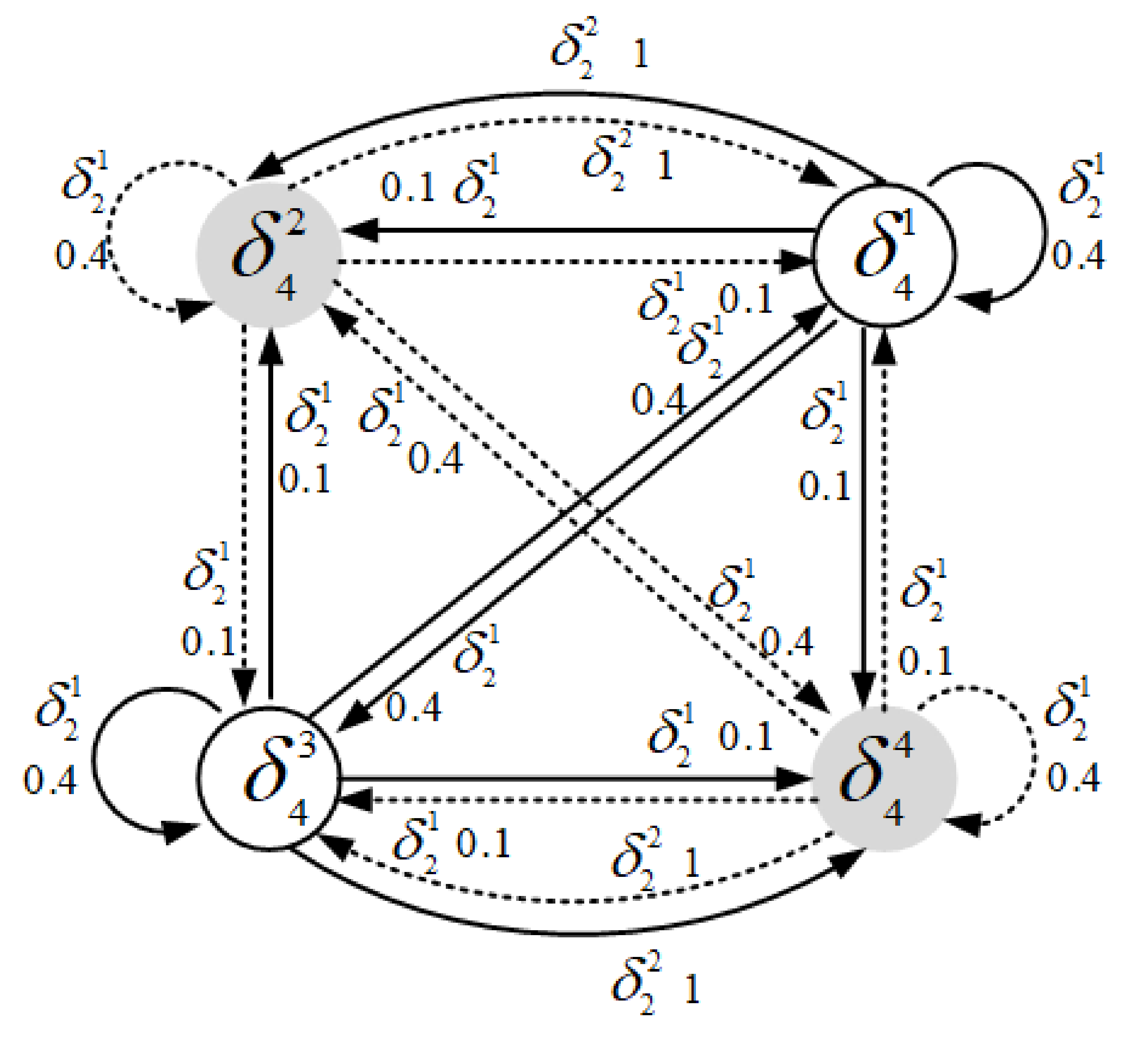
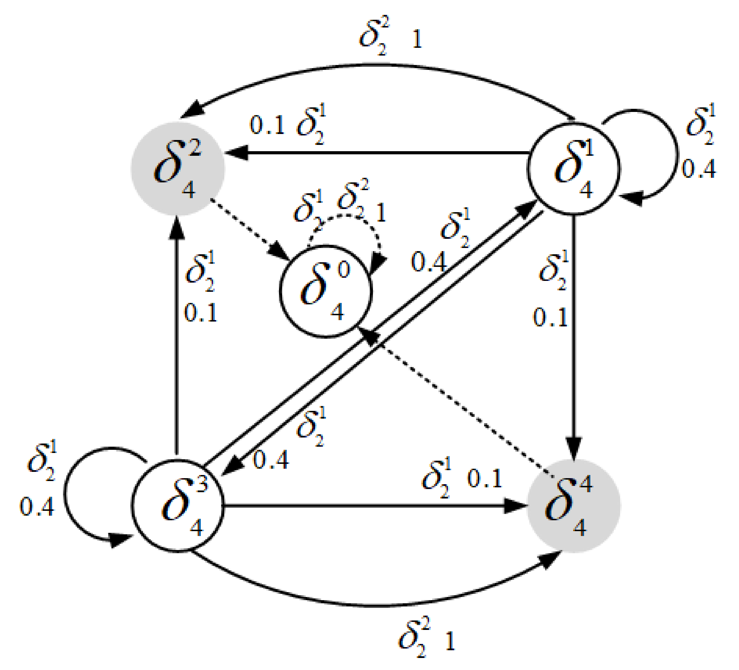
3.1. State Transfer Graph

STG reconstruction is the primary approach used in finite-time set reachability analysis. For any subset $\mathcal{M}\subset {\Delta }_{2^{KN}}$, the indicator matrix of $\mathcal{M}$ is expressed as ${\mathbf{D}}_{\mathcal{M}}$,

$$Co{l}_j\left({\mathbf{D}}_{\mathcal{M}}\right):=\left\{\begin{array}{cc}{\delta }_{2^{KN}}^j,\hfill & \mathrm{if}{\delta }_{2^{KN}}^j\in \mathcal{M},\hfill \\ {\delta }_{2^{KN}}^0,\hfill & \mathrm{otherwise},\hfill \end{array}\right.$$

where ${\mathbf{D}}_{\mathcal{M}}\in {\mathcal{B}}_{2^{KN}\times 2^{KN}}$.

Different from the STG in [42], we define ${\widehat{\mathbf{D}}}_{\mathcal{M}}$ as follows:

$${\widehat{\mathbf{D}}}_{\mathcal{M}}={\left[\begin{array}{cccc}{\mathbf{D}}_{\mathcal{M}}& 0& \cdots & 0\\ 0& {\mathbf{D}}_{\mathcal{M}}& \cdots & 0\\ ⋮& ⋮& \ddots & ⋮\\ 0& 0& \cdots & {\mathbf{D}}_{\mathcal{M}}\end{array}\right]}_{2^{(m+KN)}\times 2^{(m+KN)}}$$

Then, ${\widehat{\mathbf{D}}}_{{\mathcal{M}}_d^c}$ and ${\widehat{\mathbf{D}}}_{{\tilde{\mathcal{M}}}_d^c}$ can be described as follows:

$${\widehat{\mathbf{D}}}_{{\mathcal{M}}_d^c}:={\left[\begin{array}{cccc}{\mathbf{D}}_{{\mathcal{M}}_d^c}& 0& \cdots & 0\\ 0& {\mathbf{D}}_{{\mathcal{M}}_d^c}& \cdots & 0\\ ⋮& ⋮& \ddots & ⋮\\ 0& 0& \cdots & {\mathbf{D}}_{{\mathcal{M}}_d^c}\end{array}\right]}_{2^{(m+KN)}\times 2^{(m+KN)}}$$

$${\widehat{\mathbf{D}}}_{{\tilde{\mathcal{M}}}_d^c}:={\left[\begin{array}{cccc}{\mathbf{D}}_{{\tilde{\mathcal{M}}}_d^c}& 0& \cdots & 0\\ 0& {\mathbf{D}}_{{\tilde{\mathcal{M}}}_d^c}& \cdots & 0\\ ⋮& ⋮& \ddots & ⋮\\ 0& 0& \cdots & {\mathbf{D}}_{{\tilde{\mathcal{M}}}_d^c}\end{array}\right]}_{2^{(m+KN)}\times 2^{(m+KN)}}$$

It should be noted that the dimensions of ${\mathcal{M}}_d^c$ and ${\tilde{M}}_d^c$ are inconsistent. ${\mathcal{M}}_d^c$ is the supplementary set of the overall target subset ${\mathcal{M}}_d$ in ${\Delta }_{2^{KN}}$, and ${\tilde{M}}_d^c$ is the supplementary set of the global target subset ${\tilde{M}}_d$ in ${\Delta }_{2^n}$.

Here, the state spaces ${\Delta }_{2^{KN}}$ and ${\Delta }_{2^n}$ could be extended to ${\Delta }_{2^{KN}}^0$ and ${\Delta }_{2^n}^0$, where ${\Delta }_{2^{KN}}^0:={\Delta }_{2^{KN}}\cup \left\{{\delta }_{2^{KN}}^0\right\}$, ${\Delta }_{2^n}^0:={\Delta }_{2^n}\cup \left\{{\delta }_{2^n}^0\right\}$, and construct the RLDS as

$$\left\{\begin{array}{c}\begin{array}{cc}\widehat{x}(t+1)\hfill & =L\eta \left(t\right){\widehat{\mathbf{D}}}_{{\mathcal{M}}_d^c}u\left(t\right)\widehat{x}\left(t\right),\hfill \end{array}\hfill \\ \begin{array}{cc}\check{x}(t+1)\hfill & =\tilde{L}\eta \left(t\right){\widehat{\mathbf{D}}}_{{\tilde{\mathcal{M}}}_d^c}u\left(t\right)\widehat{x}\left(t\right),\hfill \end{array}\hfill \end{array}\right.$$

(7)

where $\widehat{x}\left(t\right)\in {\Delta }_{2^{KN}}^0$, $\check{x}\left(t\right)\in {\Delta }_{2^n}^0$, and for any $u\left(t\right)\in {\Delta }_{2^m}$, it follows that $L\eta \left(t\right){\widehat{\mathbf{D}}}_{{\mathcal{M}}_d^c}u\left(t\right)\widehat{x}\left(t\right)\ne {\delta }_{2^{KN}}^0$ iff $\widehat{x}\left(t\right)\in {\mathcal{M}}_d^c$ and $\tilde{L}\eta \left(t\right){\widehat{\mathbf{D}}}_{{\tilde{\mathcal{M}}}_d^c}u\left(t\right)\widehat{x}\left(t\right)\ne {\delta }_{2^n}^0$ iff $x\left(t\right)\in {\tilde{\mathcal{M}}}_d^c$.

Remark 2.

Different from [18], the RLDS proposed in this paper is an extension of PMBCN rather than one-layer probabilistic Boolean network. Moreover, the definition of indicator matrix is also different from [18].

The PBMCNs (4) can be transformed into RLDS (7) by the indicator matrices ${\widehat{\mathbf{D}}}_{{\mathcal{M}}_d^c}$ and ${\widehat{\mathbf{D}}}_{{\tilde{\mathcal{M}}}_d^c}$. Next, the transformation relationship between the PBMCNs (4) and RLDS (7) is given by using the STG reconstruction technique.

Since ${\mathrm{p}}^{\sigma }$ is the probability distribution vector of $\eta \left(t\right)$, using (7), we define the one-step nonzero state transition probability matrix of RLDS (7), $P^{\widehat{x}}$ and $P^{\check{x}}$

$$\begin{array}{c}{P}^{\widehat{x}}=L⋉{\mathrm{p}}^{\sigma }⋉\widehat{}\}{\mathbf{D}}_{{\mathcal{M}}_d^c}=P^x\widehat{}\}{\mathbf{D}}_{{\mathcal{M}}_d^c},\hfill \\ P^{\check{x}}=\tilde{L}⋉{\mathrm{p}}^{\sigma }⋉\widehat{}\}{\mathbf{D}}_{{\tilde{\mathcal{M}}}_d^c}=P^{\tilde{x}}\widehat{}\}{\mathbf{D}}_{{\tilde{\mathcal{M}}}_d^c}.\hfill \end{array}$$

(8)

The one-step nonzero state overall transition probability matrix $P^{\widehat{x}}$ and the one-step nonzero state global transition probability matrix $P^{\check{x}}$ of RLDS (7) are divided into $2^m$ matrices as follows:

$$\begin{array}{c}{P}^{\widehat{x}}=[P_{\left(1\right)}^{\widehat{x}}{P}_{\left(2\right)}^{\widehat{x}}\dots P_{\left(2^m\right)}^{\widehat{x}}],\hfill \\ P^{\check{x}}=[P_{\left(1\right)}^{\check{x}}{P}_{\left(2\right)}^{\check{x}}\dots P_{\left(2^m\right)}^{\check{x}}],\hfill \end{array}$$

(9)

where $P_{\left(q\right)}^{\widehat{x}}\in {\Delta }_{2^{KN}}^0$ and $P_{\left(q\right)}^{\check{x}}\in {\Delta }_{2^n}^0$, then, we have

${\left[P_{\left(q\right)}^{\widehat{x}}\right]}_{ij}:=\mathrm{Pr}\{\widehat{x}(t+1)={\delta }_{2^{KN}}^i|\widehat{x}\left(t\right)={\delta }_{2^{KN}}^j\},i,j\in [1,2^{KN}],$

${\left[P_{\left(q\right)}^{\check{x}}\right]}_{ij}:=\mathrm{Pr}\{\check{x}(t+1)={\delta }_{2^n}^i|\widehat{x}\left(t\right)={\delta }_{2^{KN}}^j\},i\in [1,2^n]$ and $j\in [1,2^{KN}]$

where $q\in [1,2^m]$, $P_{\left(q\right)}^{\widehat{x}}$ and $P_{\left(q\right)}^{\check{x}}$ denote the $q$-th block of the nonzero state transition probability matrices $P^{\widehat{x}}$ and $P^{\check{x}}$, respectively.

Then, the one-step overall and global transition probabilities between the states of RLDS (7) can be obtained as follows:

$$\begin{array}{cc}{\widehat{p}}_{ij}\hfill & ={\left[P_{\left(q\right)}^{\widehat{x}}\right]}_{ij}=\mathrm{Pr}\{\widehat{x}(t+1)={\delta }_{2^{KN}}^i\mid \widehat{x}\left(t\right)={\delta }_{2^{KN}}^j\}\hfill \\ \hfill & =\left\{\begin{array}{cc}{\left[P_{\left(q\right)}^{\widehat{x}}\right]}_{ij},& i,j\in [1,2^{KN}];\hfill \\ 0,& i=0,j\in {\Lambda }_d^c;\hfill \\ 1,& i=0,j\in \left\{0\right\}\cup {\Lambda }_d;\hfill \\ 0,& i\ne 0,j=0.\hfill \end{array}\right.\hfill \end{array}$$

(10)

$$\begin{array}{cc}{\check{p}}_{ij}\hfill & ={\left[P_{\left(q\right)}^{\check{x}}\right]}_{ij}=\mathrm{Pr}\{\check{x}(t+1)={\delta }_{2^n}^i\mid \widehat{x}\left(t\right)={\delta }_{2^{KN}}^j\}\hfill \\ \hfill & =\left\{\begin{array}{cc}{\left[P_{\left(q\right)}^{\check{x}}\right]}_{ij},& i\in [1,2^n],j\in [1,2^{KN}];\hfill \\ 0,& i=0,j\in {\tilde{\Lambda }}_d^c;\hfill \\ 1,& i=0,j\in \left\{0\right\}\cup {\tilde{\Lambda }}_d;\hfill \\ 0,& i\ne 0,j=0.\hfill \end{array}\right.\hfill \end{array}$$

(11)

Here ${\Lambda }_d$ and ${\Lambda }_d^c$ are the index sets of ${\mathcal{M}}_d$ and ${\mathcal{M}}_d^c$, respectively, i.e., ${\mathcal{M}}_d=\{{\delta }_{2^{KN}}^i\mid i\in {\Lambda }_d\}$ and ${\mathcal{M}}_d^c=\{{\delta }_{2^{KN}}^i\mid i\in {\Lambda }_d^c\}$. ${\tilde{\Lambda }}_d$ and ${\tilde{\Lambda }}_d^c$ are the index sets of ${\tilde{\mathcal{M}}}_d$ and ${\tilde{\mathcal{M}}}_d^c$, respectively, i.e., ${\tilde{\mathcal{M}}}_d=\{{\delta }_{2^n}^i\mid i\in {\tilde{\Lambda }}_d\}$ and ${\tilde{\mathcal{M}}}_d^c=\{{\delta }_{2^n}^i\mid i\in {\tilde{\Lambda }}_d^c\}$.

In fact, RLDS (7) can be obtained by reconstructing the STG of the PBMCNs (4). The global STG of RLDS is an edge-labeled graph ($\mathcal{X}$, $\epsilon$), where

1.

$\mathcal{X}$=${\mathcal{X}}_1$∪${\mathcal{X}}_2$ is the set of nodes. For the PBMCNs (4), ${\mathcal{X}}_{1\left(4\right)}$=${\Delta }_{2^{KN}}$ and ${\mathcal{X}}_{2\left(4\right)}$=${\Delta }_{2^n}$. For RLDS (7), ${\mathcal{X}}_{1\left(7\right)}$=${\Delta }_{2^{KN}}^0$ and ${\mathcal{X}}_{2\left(7\right)}$=${\Delta }_{2^n}^0$.

2.

$\epsilon \subseteq$${\mathcal{X}}_1$×${\mathcal{X}}_2$$\times [0,1]\times {\delta }_{2^m}^s$ denote the set of labled edges. $({\delta }_{2^{KN}}^j,{\delta }_{2^n}^i$, $p_{ij},{\delta }_{2^m}^s)\in \epsilon$ represents the system travels from ${\delta }_{2^{KN}}^j$ to ${\delta }_{2^n}^i$ with a probability $p_{ij}$ under the control ${\delta }_{2^m}^s$, denote by ${\delta }_{2^{KN}}^j\underset{{\delta }_{2^m}^s}{\overset{p_{ij}}{\to }}{\delta }_{2^n}^i$.

The STGs of PBMCNs (4) and RLDS (7) are represented by $({\mathcal{X}}_{\left(4\right)},{\epsilon }_{\left(4\right)})$ and $({\mathcal{X}}_{\left(7\right)},{\epsilon }_{\left(7\right)})$, respectively. Further, ${\mathcal{X}}_{1\left(7\right)}$=${\mathcal{X}}_{1\left(4\right)}$$\cup \left\{{\delta }_{2^{KN}}^0\right\}$, ${\mathcal{X}}_{2\left(7\right)}$=${\mathcal{X}}_{2\left(4\right)}$$\cup \left\{{\delta }_{2^n}^0\right\}$, and ${\epsilon }_{\left(7\right)}={\epsilon }_1\cup {\epsilon }_2\cup {\epsilon }_3$, where

• ${\epsilon }_1=\{({\delta }_{2^{KN}}^j,{\delta }_{2^n}^i,p_{ij},{\delta }_{2^m}^s)\in {\epsilon }_{\left(4\right)}\mid j\in {\Lambda }_d^c,i\in [1,2^n]\},$
• ${\epsilon }_2=\{({\delta }_{2^{KN}}^j,{\delta }_{2^n}^0,1,{\delta }_{2^m}^s)\mid j\in {\Lambda }_d\},$
• ${\epsilon }_3=({\delta }_{2^{KN}}^0,{\delta }_{2^n}^0,1,{\delta }_{2^m}^s).$

The STG of RLDS (7) may be determined intuitively from the STG of PBMCNs (4) as follows:

• The edge starting from ${\tilde{\mathcal{M}}}_d^c$ in $({\mathcal{X}}_{\left(4\right)},{\epsilon }_{\left(4\right)})$ stay unaltered.
• The edge starting from ${\tilde{\mathcal{M}}}_d$ in $({\mathcal{X}}_{\left(4\right)},{\epsilon }_{\left(4\right)})$ are substituted with the edges in $({\mathcal{X}}_{\left(7\right)},{\epsilon }_{\left(7\right)})$ directed toward ${\delta }_{2^n}^0$ with probability one.
• The edge $({\delta }_{2^{KN}}^0,{\delta }_{2^n}^0,1,{\delta }_{2^m}^s)$ is added.

For the overall state, the transition rule of STG from PBMCNs (4) to RLDS (7) conforms with the overall state, but the set of the overall state nodes is $\mathcal{X}$=${\Delta }_{2^{KN}}$.

In addition, we utilize a numerical example to demonstrate the above-mentioned procedure.

Example 1.

Consider the PBMCNs that has a one-step transition probability matrix $P^{\tilde{x}}$.

$$P^{\tilde{x}}=\left[\begin{array}{cccccccc}0.4& 0.1& 0.4& 0.1& 0& 1& 0& 0\\ 0.1& 0.4& 0.1& 0.4& 1& 0& 0& 0\\ 0.4& 0.1& 0.4& 0.1& 0& 0& 0& 1\\ 0.1& 0.4& 0.1& 0.4& 0& 0& 1& 0\end{array}\right]$$

Supposing that ${\tilde{\mathcal{M}}}_d=\{{\delta }_4^2,{\delta }_4^4\}$, we can obtain ${\tilde{\mathcal{M}}}_d^c=\{{\delta }_4^1,{\delta }_4^3\}$. Then, ${\widehat{\mathbf{D}}}_{{\tilde{\mathcal{M}}}_d^c}={\delta }_8\left[10305070\right]$. The STG of the PBMCNs is shown in Figure 1.

Here ${\tilde{x}}_i\in {\tilde{\mathcal{M}}}_d$ are represented by the gray nodes, and the dashed arrows denote the edges that emerge from ${\tilde{\mathcal{M}}}_d$. The one-step global nonzero state transition probability matrix of the resulting RLDS (7) is presented as

$$P^{\check{x}}=\left[\begin{array}{cccccccc}0.4& 0& 0.4& 0& 0& 0& 0& 0\\ 0.1& 0& 0.1& 0& 1& 0& 0& 0\\ 0.4& 0& 0.4& 0& 0& 0& 0& 0\\ 0.1& 0& 0.1& 0& 0& 0& 1& 0\end{array}\right]$$

Figure 2 shows the STG of the RLDS.

3.2. Finite-Time Set Reachability with Probability One

The set reachability of PBMCNs is investigated and characterized in this section. First, we introduce a lemma for the set reachability of PBMCNs.

Lemma 4.

Assume that ${\mathcal{M}}_0\subset {\Delta }_{2^{KN}}$ is an initial subset, ${\mathcal{M}}_d\subset {\Delta }_{2^{KN}}$ is a overall target subset and ${\tilde{\mathcal{M}}}_d\subset {\Delta }_{2^n}$ is a global target subset.

1.

An input sequence $\left\{\mathit{u}\right(t),t=0,1,\dots ,\gamma -1\}$ exists such that ${\mathcal{M}}_d$ is overall reachable with probability one from ${\mathcal{M}}_0$ on $[0:\gamma -1]$ for PBMCNs (4) if and only if ${\delta }_{2^{KN}}^0$ is overall reachable with probability one from ${\mathcal{M}}_0$ on $[1:\gamma ]$ for RLDS (7).

2.

An input sequence $\left\{\mathit{u}\right(t),t=0,1,\dots ,\gamma -1\}$ exists such that ${\tilde{M}}_d$ is global reachable with probability one from ${\mathcal{M}}_0$ on $[0:\gamma -1]$ for PBMCNs (4) if and only if ${\delta }_{2^n}^0$ is global reachable with probability one from ${\mathcal{M}}_0$ on $[1:\gamma ]$ for RLDS (7).

Proof. 

Assume that $x_0\in {\mathcal{M}}_0$ is the initial state, $\widehat{x}(t,x_0)$ is the overall state to RLDS (7), $\check{x}(t,x_0)$ is the global state to RLDS (7) and there exists an input sequence $\left\{\mathit{u}\right(t),t=0,1,\dots ,$$\gamma$$-1\}$. It holds that

$$\begin{array}{cc}& \mathrm{Pr}\{\exists \xi \in [0:t-1],s.t.x(\xi ;\eta ,x_0)\in {\mathcal{M}}_d\}\hfill \\ \hfill & =\mathrm{Pr}\{\{x_0\in {\mathcal{M}}_d\}\cup \{x(1;\eta ,x_0)\in {\mathcal{M}}_d\}\cup \dots \cup \{x(\xi ;\eta ,x_0)\in {\mathcal{M}}_d\}\}\hfill \\ \hfill & =\mathrm{Pr}\left\{\bigcup _{j=1}^t\{\widehat{x}(j;\eta ,x_0)={\delta }_{2^{KN}}^0\}\right\}\hfill \\ \hfill & =\mathrm{Pr}\{\exists \xi \in [1:t],s.t.\widehat{x}(\xi ;\eta ,x_0)={\delta }_{2^{KN}}^0\}\hfill \end{array}$$

Then, we are able to easily verify that, for any $x_0\in {\mathcal{M}}_0$, there exists an input sequence $\left\{\mathit{u}\right(t),t=0,1,\dots ,$$\gamma$$-1\}$, such that (5) and (6) are equivalent to

$$\mathrm{Pr}\{\exists \xi \in [1:\gamma ],s.t.\widehat{x}(\xi ;\eta ,x_0)={\delta }_{2^{KN}}^0\}=1$$

(12)

and

$$\mathrm{Pr}\{\exists \xi \in [1:\gamma ],s.t.\check{x}(\xi ;\eta ,x_0)={\delta }_{2^n}^0\}=1$$

(13)

respectively. Thus, the claims hold. □

Lemma 5.

• The ξ step overall transition probability from any state to ${\delta }_{2^{KN}}^0$ is non-decreasing as ξ increases, i.e.,

  $$\begin{array}{cc}& \mathrm{Pr}\{\widehat{x}(\xi +1)={\delta }_{2^{KN}}^0\mid \widehat{x}\left(0\right)={\delta }_{2^{KN}}^j\}\ge \mathrm{Pr}\{\widehat{x}\left(\xi \right)={\delta }_{2^{KN}}^0\mid \widehat{x}\left(0\right)={\delta }_{2^{KN}}^j\}\hfill \end{array}$$

  (14)
• The ξ step global transition probability from any state to ${\delta }_{2^n}^0$ is non-decreasing as ξ increases, i.e.,

  $$\begin{array}{cc}& \mathrm{Pr}\{\check{x}(\xi +1)={\delta }_{2^n}^0\mid \widehat{x}\left(0\right)={\delta }_{2^{KN}}^j\}\ge \mathrm{Pr}\{\check{x}\left(\xi \right)={\delta }_{2^n}^0\mid \widehat{x}\left(0\right)={\delta }_{2^{KN}}^j\}\hfill \end{array}$$

  (15)

Moreover, due to

$$\begin{array}{cc}\widehat{x}\left(\gamma \right)\hfill & =P^{\widehat{x}}u(\gamma -1)\widehat{x}(\gamma -1)\hfill \\ \hfill & =P^{\widehat{x}}{W}_{[2^{KN},2^m]}\widehat{x}(\gamma -1)u(\gamma -1)\hfill \\ \hfill & ={\left(P^{\widehat{x}}{W}_{[2^{KN},2^m]}\right)}^2\widehat{x}(\gamma -2)u(\gamma -2)u(\gamma -1)\hfill \\ \hfill & =\dots \hfill \\ \hfill & ={\left(P^{\widehat{x}}{W}_{[2^{KN},2^m]}\right)}^{\gamma }\widehat{x}\left(0\right)u\left(0\right)u\left(1\right)\dots u(\gamma -2)u(\gamma -1)\hfill \\ \hfill & ={\left(P^{\widehat{x}}{W}_{[2^{KN},2^m]}\right)}^{\gamma }{W}_{[2^{m\gamma },2^{KN}]}u\left(0\right)u\left(1\right)\dots u(\gamma -2)u(\gamma -1)\widehat{x}\left(0\right)\hfill \end{array}$$

and

$$\begin{array}{cc}\check{x}\left(\gamma \right)\hfill & =P^{\check{x}}u(\gamma -1)\widehat{x}(\gamma -1)\hfill \\ \hfill & =P^{\check{x}}{W}_{[2^{KN},2^m]}\widehat{x}(\gamma -1)u(\gamma -1)\hfill \\ \hfill & =\left(P^{\check{x}}{W}_{[2^{KN},2^m]}\right)\left(P^{\widehat{x}}{W}_{[2^{KN},2^m]}\right)\widehat{x}(\gamma -2)u(\gamma -2)u(\gamma -1)\hfill \\ \hfill & =\dots \hfill \\ \hfill & =\left(P^{\check{x}}{W}_{[2^{KN},2^m]}\right){\left(P^{\widehat{x}}{W}_{[2^{KN},2^m]}\right)}^{\gamma -1}\widehat{x}\left(0\right)u\left(0\right)u\left(1\right)\dots u(\gamma -2)u(\gamma -1)\hfill \\ \hfill & =\left(P^{\check{x}}{W}_{[2^{KN},2^m]}\right){\left(P^{\widehat{x}}{W}_{[2^{KN},2^m]}\right)}^{\gamma -1}{W}_{[2^{m\gamma },2^{KN}]}u\left(0\right)u\left(1\right)\dots u(\gamma -2)u(\gamma -1)\widehat{x}\left(0\right)\hfill \end{array}$$

we define $\gamma$-step nonzero state transition probability matix, $\widehat{Q}$ and $\check{Q}$, by

$$\begin{array}{c}\widehat{Q}={\left(P^{\widehat{x}}{W}_{[2^{KN},2^m]}\right)}^{\gamma }{W}_{[2^{m\gamma },2^{KN}]},\hfill \\ \check{Q}=\left(P^{\check{x}}{W}_{[2^{KN},2^m]}\right){\left(P^{\widehat{x}}{W}_{[2^{KN},2^m]}\right)}^{\gamma -1}{W}_{[2^{m\gamma },2^{KN}]}.\hfill \end{array}$$

(16)

The $\gamma$-step nonzero state overall transition probability matrix $\widehat{Q}$ and the $\gamma$-step nonzero state global transition probability matrix $\check{Q}$ of RLDS (7) are divided into $2^{m\gamma }$ matrices as follows:

$$\begin{array}{c}\widehat{Q}=[{\widehat{Q}}_{\left(1\right)}{\widehat{Q}}_{\left(2\right)}\dots {\widehat{Q}}_{\left(2^{m\gamma }\right)}],\hfill \\ \check{Q}=[{\check{Q}}_{\left(1\right)}{\check{Q}}_{\left(2\right)}\dots {\check{Q}}_{\left(2^{m\gamma }\right)}]\hfill \end{array}$$

(17)

The symbol ${\displaystyle \underset{s}{\bigwedge }}$ can be defined as follows:

$$\left\{\begin{array}{c}Co{l}_j\left({\widehat{Q}}_q\right){\displaystyle \underset{s}{\bigwedge }}{\delta }_{2^{KN}}^0={\delta }_{2^{KN}}^0,\hfill \\ Co{l}_j\left({\widehat{Q}}_q\right){\displaystyle \underset{s}{\bigwedge }}{\delta }_{2^{KN}}^k=Co{l}_j\left({\widehat{Q}}_q\right),\hfill & k\in [1,2^{KN}]\hfill \end{array}\right.$$

In the same way, we can obtain

$$\left\{\begin{array}{c}Co{l}_j\left({\check{Q}}_q\right){\displaystyle \underset{s}{\bigwedge }}{\delta }_{2^n}^0={\delta }_{2^n}^0,\hfill \\ Co{l}_j\left({\check{Q}}_q\right){\displaystyle \underset{s}{\bigwedge }}{\delta }_{2^n}^k=Co{l}_j\left({\check{Q}}_q\right),\hfill & k\in [1,2^n]\hfill \end{array}\right.$$

Theorem 1.

For PBMCNs (4), suppose that ${\mathcal{M}}_0=\{{\delta }_{2^{KN}}^j\mid j\in {\Lambda }_0\}$, where ${\Lambda }_0$ is a subset of $[1:2^{KN}]$. Then, the following two statements hold.

1.

An input sequence $\left\{\mathit{u}\right(t),t=0,1,\dots ,\gamma -1\}$ exists such that ${\mathcal{M}}_d$ is overall reachable with probability one from ${\mathcal{M}}_0$ on $[0:\gamma -1]$ if and only if

$$Co{l}_j\left[{{\displaystyle \underset{s}{\bigwedge }}}_{q=1}^{2^{m\gamma }}{\widehat{Q}}_{\left(q\right)}\right]={\delta }_{2^{KN}}^0,\forall j\in {\Lambda }_0.$$

2.

An input sequence $\left\{\mathit{u}\right(t),t=0,1,\dots ,\gamma -1\}$ exists such that ${\tilde{\mathcal{M}}}_d$ is global reachable with probability one from ${\mathcal{M}}_0$ on $[0:\gamma -1]$ if and only if

$$Co{l}_j\left[{{\displaystyle \underset{s}{\bigwedge }}}_{q=1}^{2^{m\gamma }}{\check{Q}}_{\left(q\right)}\right]={\delta }_{2^n}^0,\forall j\in {\tilde{\Lambda }}_0.$$

Proof. 

First, we demonstrate that the necessary condition is satisfied. Known as ${\mathcal{M}}_d$, it is overall reachable with probability one from ${\mathcal{M}}_0$ on $[0,$$\gamma$$-1]$. Then, for any $x_0={\delta }_{2^{KN}}^j$ and $t\ge 0$, there exists an input sequence $\left\{\mathit{u}\right(t),t=0,1,\dots ,$$\gamma$$-1\}$ such that

$$\begin{array}{cc}& \mathrm{Pr}\{\exists \xi \in [0:t-1],s.t.\widehat{x}(\xi ;\eta ,x_0)\in {\mathcal{M}}_d\}\hfill \\ \hfill & =\mathrm{Pr}\{\exists \xi \in [1:t],s.t.,\widehat{x}(\xi ;\eta ,x_0)={\delta }_{2^{KN}}^0\}\hfill \\ \hfill & =\mathrm{Pr}\{\widehat{x}(t;\eta ,x_0)={\delta }_{2^{KN}}^0\}\hfill \\ \hfill & =1\hfill \end{array}$$

Since

$$\mathrm{Pr}\{\widehat{x}(t;\eta ,x_0)={\delta }_{2^{KN}}^0\}=1-\sum _{i=1}^{2^{KN}}{\left[{\widehat{Q}}_{\left(q\right)}\right]}_{ij}=1$$

for which there exists an input sequence $\left\{\mathit{u}\right(t),t=0,1,\dots ,$$\gamma$$-1\}$ such that

$$\begin{array}{c}\sum _{i=1}^{2^{KN}}{\left[{\widehat{Q}}_{\left(q\right)}\right]}_{ij}=0\hfill \end{array}$$

Then, we have

$$\begin{array}{c}Co{l}_j\left[{\widehat{Q}}_{\left(q\right)}\right]={\delta }_{2^{KN}}^0\hfill \end{array}$$

Further, we obtain

$$\begin{array}{c}Co{l}_j\left[{{\displaystyle \underset{s}{\bigwedge }}}_{q=1}^{2^{m\gamma }}\left[{\widehat{Q}}_{\left(q\right)}\right]\right]={\delta }_{2^{KN}}^0\forall j\in {\Lambda }_0\hfill \end{array}$$

Next, we prove the sufficiency condition holds. For any $j\in {\Lambda }_0$, we have $Co{l}_j\left[{{\displaystyle \underset{s}{\bigwedge }}}_{q=1}^{2^{m\gamma }}\left[{\widehat{\mathrm{Q}}}_{\left(q\right)}\right]\right]={\delta }_{2^{KN}}^0$. Then, we are able to easily verify that there exists an input sequence $\mathit{u}$ such that

$$\begin{array}{c}Co{l}_j\left[{\widehat{Q}}_{\left(q\right)}\right]={\delta }_{2^{KN}}^0\hfill \end{array}$$

which is

$$\begin{array}{cc}& 1-\sum _{i=1}^{2^{KN}}{\left[\left({\widehat{Q}}_{\left(q\right)}\right)\right]}_{ij}=1\hfill \end{array}$$

(18)

Then, (18) becomes

$$\begin{array}{c}\mathrm{Pr}\{\widehat{x}(\gamma +1)={\delta }_{2^{KN}}^0\mid x\left(0\right)={\delta }_{2^{KN}}^j\}=1\hfill \end{array}$$

Consequently, there exists an input sequence $\left\{\mathit{u}\right(t),t=0,1,\dots ,$$\gamma$$-1\}$ such that ${\mathcal{M}}_d$ is overall reachable with probability one from ${\mathcal{M}}_0$ on $[0,$$\gamma$$-1]$. Similarly, we can prove Conclusion 2, no need to repeat the arguments. □

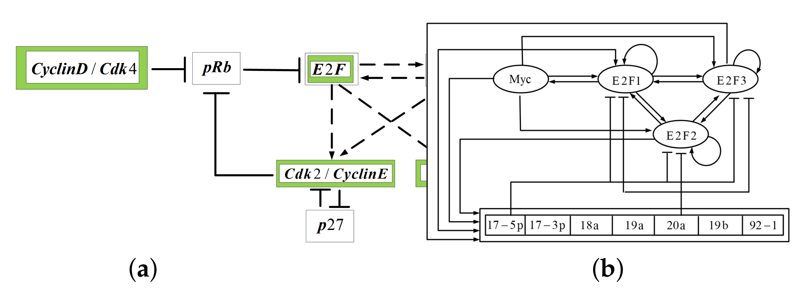
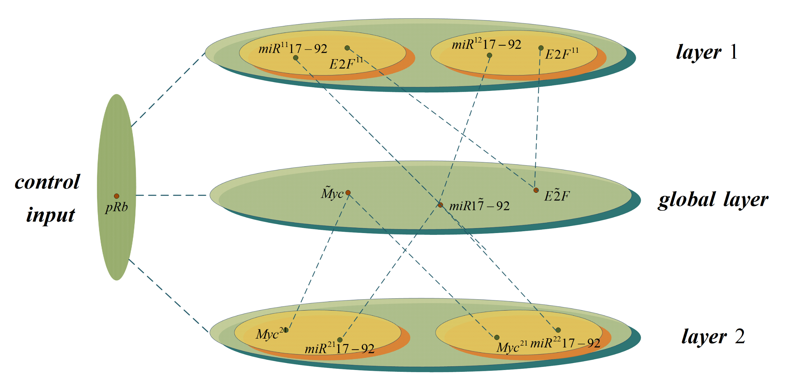
4. Result and Discussion

The cell cycle of eukaryotes consists of four phases generally: G1, S, G2 and M phases. At this point, the controllable cancer network [44] is formed by a portion of key molecules in the G1/S phase as shown in Figure 3. The dotted arrows refer to induced gene expression. The E2F protein, for example, stimulates the expression of its own gene. The expression of suppressor genes is indicated by hammerheads.

The proliferation and apoptosis of cells are regulated by transcription factors E2F and Myc in the cancer network. According to the particular expression status of cells, they fulfill the roles of tumor suppressor gene and oncogene. The microRNA, called miR-17-92, regulates E2F and Myc in the process of transcription. Meanwhile, pRb also regulates E2F. On the contrary, transcription of miR-17-92 is also induced by E2F and Myc. Under the regulation of this interaction, miR-17-92 is expressed as a tumor inhibitor or a tumor gene, severally. As a result, the cancer network (Figure 3) was added to a straightforward regulatory network [45], including E2F, Myc, and miR-17-92 (Figure 4). In this way, the PBMCN can simulate the simplified network more effectively, and the resulting network model is shown in Figure 4.

The networks are summarized as follows:

$$l=1:\left\{\begin{array}{c}E2F(t+1)=f_{E2F}(E2F\left(t\right),mi{R}_1\left(t\right),pRb\left(t\right)),\hfill \\ mi{R}_1(t+1)=f_{mi{R}_1}^1(E2F\left(t\right),mi{R}_1\left(t\right),pRb\left(t\right))\hfill \end{array}\right.$$

$$l=2:\left\{\begin{array}{c}mi{R}_2(t+1)=f_{mi{R}_2}^2(mi{R}_2\left(t\right),Myc\left(t\right),pRb\left(t\right)),\hfill \\ Myc(t+1)=f_{mi{R}_2}^2(mi{R}_2\left(t\right),Myc\left(t\right),pRb\left(t\right))\hfill \end{array}\right.$$

For simplicity, E2F, $mi{R}_1$, $mi{R}_2$, Myc and pRb are represented by $x_1^1,x_2^1,x_2^2,x_3^2$ and $u\left(t\right)$, respectively. The specific variables involved are defined as follows:

• $x_1^1$: Transcription factor involved in gene transcription;
• $x_3^2$: Transcription factor involved in gene transcription;
• $x_2^1,x_2^2$: Non-coding RNA cluster;
• $u\left(t\right)$: Retinoblastoma protein;
• $f_{11}^1$: The transcription of miRNA-17-92 is promoted, allowing E2F to enter the cancerous regions under the regulation of retinoblastoma protein;
• $f_{21}^1$: The expression of oncogenes is promoted by E2F;
• $f_{22}^1$: The expression of oncogenes is inhibited by E2F, and tumor suppressor genes are expressed by E2F;
• $f_{21}^1$: The expression of oncogenes is promoted by Myc;
• $f_{22}^2$: The expression of oncogenes is inhibited by Myc, and tumor suppressor genes are expressed by Myc;
• $f_{31}^2$: The transcription of miRNA-17-92 is promoted, allowing Myc to enter the cancerous regions.

The logic function $f_{11}^1$ can be selected with the probabilities for $x_1^1$.

$$x_1^1(t+1)=f_{11}^1(x_1^1\left(t\right),x_2^1\left(t\right),u\left(t\right))=x_2^1\left(t\right)\wedge u\left(t\right).$$

The logic function $f_{21}^1$ and $f_{22}^1$ can be selected with the probabilities for $x_2^1$.

$$x_2^1(t+1):\left\{\begin{array}{c}{f}_{21}^1(x_1^1\left(t\right),x_2^1\left(t\right),u\left(t\right))=x_1^1\left(t\right),\hfill \\ f_{22}^1(x_1^1\left(t\right),x_2^1\left(t\right),u\left(t\right))=\neg x_1^1\left(t\right)\hfill \end{array}\right.$$

The corresponding probabilities are given: $p(f_2^1=f_{21}^1)=0.5$ and $p(f_2^1=f_{22}^1)=0.5$, respectively.

The logic function $f_{21}^2$ and $f_{22}^2$ can be selected with the probabilities for $x_2^2$.

$$x_2^2(t+1):\left\{\begin{array}{c}{f}_{21}^2(x_2^2\left(t\right),x_3^2\left(t\right),u\left(t\right))=x_3^2\left(t\right),\hfill \\ f_{22}^2(x_2^2\left(t\right),x_3^2\left(t\right),u\left(t\right))=\neg x_3^2\left(t\right)\hfill \end{array}\right.$$

The corresponding probabilities are given: $p(f_2^2=f_{21}^2)=0.5$ and $p(f_2^2=f_{22}^2)=0.5$, respectively.

The logic function $f_{31}^2$ and $f_{32}^2$ can be selected with the probabilities for $x_3^2$.

$$x_3^2(t+1)=f_{31}^2(x_2^2\left(t\right),x_3^2\left(t\right),u\left(t\right))=x_2^2\left(t\right).$$

Second, the global state layer is formulated by ${\tilde{x}}_1(t+1),{\tilde{x}}_2(t+1),{\tilde{x}}_3(t+1)$, we have

$$\left\{\begin{array}{c}{\tilde{x}}_1(t+1)=x_1^1(t+1),\hfill \\ {\tilde{x}}_2(t+1)=x_2^1(t+1)\vee x_2^2(t+1),\hfill \\ {\tilde{x}}_3(t+1)=x_3^2(t+1)\hfill \end{array}\right.$$

Here, $\neg ,\vee ,\wedge$ represent the logical functions of “negation”, “disjunction”, “conjunction”, respectively. Then, the two-layer PBCNs can be transformed into the corresponding algebraic representation. The input layers are represented as follows:

$$x_1^1(t+1)=f_{11}^1(x_1^1\left(t\right),x_2^1\left(t\right),u\left(t\right))=x_2^1\left(t\right)\wedge u\left(t\right)$$

$$x_2^1(t+1):\left\{\begin{array}{c}{f}_{21}^1(x_1^1\left(t\right),x_2^1\left(t\right),u\left(t\right))=x_1^1\left(t\right),\hfill \\ f_{22}^1(x_1^1\left(t\right),x_2^1\left(t\right),u\left(t\right))=M_n{x}_1^1\left(t\right)\hfill \end{array}\right.$$

$$x_2^2(t+1):\left\{\begin{array}{c}{f}_{21}^2(x_2^2\left(t\right),x_3^2\left(t\right),u\left(t\right))=x_3^2\left(t\right),\hfill \\ f_{22}^2(x_2^2\left(t\right),x_3^2\left(t\right),u\left(t\right))=M_n{x}_3^2\left(t\right)\hfill \end{array}\right.$$

$$x_3^2(t+1)=f_{31}^2(x_2^2\left(t\right),x_3^2\left(t\right),u\left(t\right))=x_2^2\left(t\right)$$

Next, the global state layer can be obtained as follows:

$$\left\{\begin{array}{c}{\tilde{x}}_1(t+1)=x_1^1(t+1),\hfill \\ {\tilde{x}}_2(t+1)=M_d{x}_2^1(t+1)x_2^2(t+1),\hfill \\ {\tilde{x}}_3(t+1)=x_3^2(t+1)\hfill \end{array}\right.$$

Then, there are four networks to choose from, and the corresponding probabilities of each network are shown in

Table 1. Sub-Model of PBMCNs.

∑	P
$f_{11}^1,f_{21}^1,f_{21}^2,f_{31}^2$	$1\times 0.5\times 0.5\times 1=0.25$
$f_{11}^1,f_{22}^1,f_{21}^2,f_{31}^2$	$1\times 0.5\times 0.5\times 1=0.25$
$f_{11}^1,f_{21}^1,f_{22}^2,f_{31}^2$	$1\times 0.5\times 0.5\times 1=0.25$
$f_{11}^1,f_{22}^1,f_{22}^2,f_{31}^2$	$1\times 0.5\times 0.5\times 1=0.25$

.

Based on the STP of matrix, we are able to easily obtain the overall state transition matrix L and global state transition matrix $\tilde{L}$. Suppose that ${\tilde{\mathcal{M}}}_d=\left\{{\delta }_{16}^2{\delta }_{16}^5{\delta }_{16}^8\right\}$. Then, we have

$$\begin{array}{c}L=\left[\begin{array}{cccccccccccccccc}0.25& 0.25& 0& 0& 0& 0& 0& 0& 0.25& 0.25& 0& 0& 0& 0& 0& 0\\ 0& 0& 0.25& 0.25& 0& 0& 0& 0& 0& 0& 0.25& 0.25& 0& 0& 0& 0\\ 0.25& 0.25& 0& 0& 0& 0& 0& 0& 0.25& 0.25& 0& 0& 0& 0& 0& 0\\ 0& 0& 0.25& 0.25& 0& 0& 0& 0& 0& 0& 0.25& 0.25& 0& 0& 0& 0\\ 0.25& 0.25& 0& 0& 0& 0& 0& 0& 0.25& 0.25& 0& 0& 0& 0& 0& 0\\ 0& 0& 0.25& 0.25& 0& 0& 0& 0& 0& 0& 0.25& 0.25& 0& 0& 0& 0\\ 0.25& 0.25& 0& 0& 0& 0& 0& 0& 0.25& 0.25& 0& 0& 0& 0& 0& 0\\ 0& 0& 0.25& 0.25& 0& 0& 0& 0& 0& 0& 0.25& 0.25& 0& 0& 0& 0\\ 0& 0& 0& 0& 0.25& 0.25& 0& 0& 0& 0& 0& 0& 0& 0& 0.25& 0.25\\ 0& 0& 0& 0& 0& 0& 0.25& 0.25& 0& 0& 0& 0& 0& 0& 0.25& 0.25\\ 0& 0& 0& 0& 0.25& 0.25& 0& 0& 0& 0& 0& 0& 0.25& 0.25& 0& 0\\ 0& 0& 0& 0& 0& 0& 0.25& 0.25& 0& 0& 0& 0& 0& 0& 0.25& 0.25\\ 0& 0& 0& 0& 0.25& 0.25& 0& 0& 0& 0& 0& 0& 0.25& 0.25& 0& 0\\ 0& 0& 0& 0& 0& 0& 0.25& 0.25& 0& 0& 0& 0& 0& 0& 0.25& 0.25\\ 0& 0& 0& 0& 0.25& 0.25& 0& 0& 0& 0& 0& 0& 0.25& 0.25& 0& 0\\ 0& 0& 0& 0& 0& 0& 0.25& 0.25& 0& 0& 0& 0& 0& 0& 0.25& 0.25\end{array}\right.\hfill \\ \hfill \left.\begin{array}{cccccccccccccccc}0& 0& 0& 0& 0& 0& 0& 0& 0& 0& 0& 0& 0& 0& 0& 0\\ 0& 0& 0& 0& 0& 0& 0& 0& 0& 0& 0& 0& 0& 0& 0& 0\\ 0& 0& 0& 0& 0& 0& 0& 0& 0& 0& 0& 0& 0& 0& 0& 0\\ 0& 0& 0& 0& 0& 0& 0& 0& 0& 0& 0& 0& 0& 0& 0& 0\\ 0& 0& 0& 0& 0& 0& 0& 0& 0& 0& 0& 0& 0& 0& 0& 0\\ 0& 0& 0& 0& 0& 0& 0& 0& 0& 0& 0& 0& 0& 0& 0& 0\\ 0& 0& 0& 0& 0& 0& 0& 0& 0& 0& 0& 0& 0& 0& 0& 0\\ 0& 0& 0& 0& 0& 0& 0& 0& 0& 0& 0& 0& 0& 0& 0& 0\\ 0.25& 0.25& 0& 0& 0.25& 0.25& 0& 0& 0.25& 0.25& 0& 0& 0.25& 0.25& 0& 0\\ 0& 0& 0.25& 0.25& 0& 0& 0.25& 0.25& 0& 0& 0.25& 0.25& 0& 0& 0.25& 0.25\\ 0.25& 0.25& 0& 0& 0.25& 0.25& 0& 0& 0.25& 0.25& 0& 0& 0.25& 0.25& 0& 0\\ 0& 0& 0.25& 0.25& 0& 0& 0.25& 0.25& 0& 0& 0.25& 0.25& 0& 0& 0.25& 0.25\\ 0.25& 0.25& 0& 0& 0.25& 0.25& 0& 0& 0.25& 0.25& 0& 0& 0.25& 0.25& 0& 0\\ 0& 0& 0.25& 0.25& 0& 0& 0.25& 0.25& 0& 0& 0.25& 0.25& 0& 0& 0.25& 0.25\\ 0.25& 0.25& 0& 0& 0.25& 0.25& 0& 0& 0.25& 0.25& 0& 0& 0.25& 0.25& 0& 0\\ 0& 0& 0.25& 0.25& 0& 0& 0.25& 0.25& 0& 0& 0.25& 0.25& 0& 0& 0.25& 0.25\end{array}\right]\end{array}$$

and

$$\begin{array}{c}\tilde{L}=\left[\begin{array}{cccccccccccccccc}0.75& 0.75& 0& 0& 0& 0& 0& 0& 0.75& 0.75& 0& 0& 0& 0& 0& 0\\ 0& 0& 0.75& 0.75& 0& 0& 0& 0& 0& 0& 0.75& 0.75& 0& 0& 0& 0\\ 0.25& 0.25& 0& 0& 0& 0& 0& 0& 0.25& 0.25& 0& 0& 0& 0& 0& 0\\ 0& 0& 0.25& 0.25& 0& 0& 0& 0& 0& 0& 0.25& 0.25& 0& 0& 0& 0\\ 0& 0& 0& 0& 0.75& 0.75& 0& 0& 0& 0& 0& 0& 0.75& 0.75& 0& 0\\ 0& 0& 0& 0& 0& 0& 0.75& 0.75& 0& 0& 0& 0& 0& 0& 0.75& 0.75\\ 0& 0& 0& 0& 0.25& 0.25& 0& 0& 0& 0& 0& 0& 0.25& 0.25& 0& 0\\ 0& 0& 0& 0& 0& 0& 0.25& 0.25& 0& 0& 0& 0& 0& 0& 0.25& 0.25\end{array}\right.\hfill \\ \hfill \left.\begin{array}{cccccccccccccccc}0& 0& 0& 0& 0& 0& 0& 0& 0& 0& 0& 0& 0& 0& 0& 0\\ 0& 0& 0& 0& 0& 0& 0& 0& 0& 0& 0& 0& 0& 0& 0& 0\\ 0& 0& 0& 0& 0& 0& 0& 0& 0& 0& 0& 0& 0& 0& 0& 0\\ 0& 0& 0& 0& 0& 0& 0& 0& 0& 0& 0& 0& 0& 0& 0& 0\\ 0.75& 0.75& 0& 0& 0.75& 0.75& 0& 0& 0.75& 0.75& 0& 0& 0.75& 0.75& 0& 0\\ 0& 0& 0.75& 0.75& 0& 0& 0.75& 0.75& 0& 0& 0.75& 0.75& 0& 0& 0.75& 0.75\\ 0.25& 0.25& 0& 0& 0.25& 0.25& 0& 0& 0.25& 0.25& 0& 0& 0.25& 0.25& 0& 0\\ 0& 0& 0.25& 0.25& 0& 0& 0.25& 0.25& 0& 0& 0.25& 0.25& 0& 0& 0.25& 0.25\end{array}\right]\end{array}$$

The PDV of the two-layers PBCNs as follows:

${\mathrm{p}}^{\sigma }={\left[0.250.250.250.25\right]}^T$

According to (8) and (16), we can obtain the matrix $\left[{{\displaystyle \underset{s}{\bigwedge }}}_{q=1}^{2^{m\gamma }}{\check{\mathrm{Q}}}_{\left(q\right)}\right]=\left[{{\displaystyle \underset{s}{\bigwedge }}}_{q=1}^{2^3}{\check{\mathrm{Q}}}_{\left(q\right)}\right]$ as follows:

$$\left[{{\displaystyle \underset{s}{\bigwedge }}}_{q=1}^{2^3}{\check{\mathrm{Q}}}_{\left(q\right)}\right]=\left(\begin{array}{cccccccccccccccc}0& 0& 0& 0& 0& 0& 0& 0& 0& 0& 0& 0& 0& 0& 0& 0\\ 0& 0& 0& 0& 0& 0& 0& 0& 0& 0& 0& 0& 0& 0& 0& 0\\ 0& 0& 0& 0& 0& 0& 0& 0& 0& 0& 0& 0& 0& 0& 0& 0\\ 0& 0& 0& 0& 0& 0& 0& 0& 0& 0& 0& 0& 0& 0& 0& 0\\ 0& 0& 0& 0& 0& 0& 0& 0& 0& 0& 0& 0& 0& 0& 0& 0\\ 0& 0& 0& 0& 0& 0& 0& 0& 0& 0& 0& 0& 0& 0& 0& 0\\ 0& 0& 0& 0& 0& 0& 0& 0& 0& 0& 0& 0& 0& 0& 0& 0\\ 0& 0& 0& 0& 0& 0& 0& 0& 0& 0& 0& 0& 0& 0& 0& 0\end{array}\right)$$

By observing the above matrix, it can be seen that all the column vectors of the matrix are zero vectors. Then, according to the Theorem 1, we are able to easily obtain that ${\tilde{\mathcal{M}}}_d=\{{\delta }_{16}^2,{\delta }_{16}^5,{\delta }_{16}^8\}$ is global reachable with probability one from arbitrary initial state on $[0,3]$. Thus, we can conclude the cancer network’s finite-time set reachability on the premise of ${\tilde{\mathcal{M}}}_d=\{{\delta }_{16}^2,{\delta }_{16}^5,{\delta }_{16}^8\}$.

5. Conclusions

This study investigated the finite-time set reachability of PBMCNs. For the finite-time set reachability analysis, the PBMCNs were extended to the RLDS via STG reconstruction technology. On this basis, a necessary and sufficient condition for the finite-time set reachability of PBMCNs was obtained. Finally, the proposed method was illustrated by a numerical example. The main results are as follows:

1.

Considering the systematic nature of biological models, in this paper, the PBMCNs are proposed based on the PBCNs. The model can simulate complex gene regulatory networks, such as cancer networks.

2.

In order to demonstrate the set reachability of PBMCNs, the set reachability issue of PBMCNs is transformed into the set reachability issue of RLDS by the STG reconstruction technique, and a necessary and sufficient condition for the finite-time set reachability of PBMCNs is obtained.

Although the PBMCNs proposed in this paper can simulate more complex gene regulatory networks, this model still has the limitation that the computational complexity $O(2^{KN+m}\times 2^{KN+m})$ will further complicate as the number of nodes increases. Therefore, we will focus on reducing the computational complexity of the PBMCNs in further research.

References

1. Kauffman, S.A. Metabolic stability and epigenesis in randomly constructed genetic nets. J. Theor. Biol. 1968, 22, 437–467. [Google Scholar] [CrossRef]
2. Kauffman, S.A. At home in the universe. Math. Soc. Sci. 1995, 33, 94–95. [Google Scholar]
3. Krumsiek, J.; Marr, C.; Schroeder, T.; Theis, F.J. Hierarchical differentiation of myeloid progenitors is encoded in the transcription factor network. PLoS ONE 2011, 6, e22649. [Google Scholar] [CrossRef] [PubMed] [Green Version]
4. Chang, R.; Shoemaker, R.; Wang, W. Systematic search for recipes to generate induced pluripotent stem cells. PLoS Comput. Biol. 2011, 7, e1002300. [Google Scholar] [CrossRef]
5. Flttmann, M.; Scharp, T.; Klipp, E. A stochastic model of epigenetic dynamics in somatic cell reprogramming. Front. Physiol. 2012, 3, 216. [Google Scholar] [CrossRef] [Green Version]
6. Li, H.; Wang, Y. Boolean derivative calculation with application to fault detection of combinational circuit via the semi-tensor product method. Automatica 2012, 48, 688–693. [Google Scholar] [CrossRef]
7. Liu, Z.; Wang, Y.; Li, H. New approach to derivative calculation of multi-valued logical functions with application to fault detection of digital circuits. IET Control Theory A 2014, 8, 554–560. [Google Scholar] [CrossRef]
8. Zhang, J.Y.; Wu, Y.H. A stochastic logical model-based approximate solution for energy management problem of HEVs. Sci. China Inf. Sci. 2018, 61, 1–3. [Google Scholar] [CrossRef] [Green Version]
9. Cheng, D.Z.; Qi, H.S.; Zhao, Y. An Introduction to Semi-Tensor Product of Matrices and Its Applications; World Scientific Publishing Co. Pte. Ltd.: Singapore, 2012; pp. 37–56. [Google Scholar]
10. Yu, Y.Y.; Meng, M.; Feng, J.E. Observability of Boolean networks via matrix equations. Automatica 2020, 111, 108621. [Google Scholar] [CrossRef]
11. Yu, Y.Y.; Meng, M.; Feng, J.E.; Chen, G. Observability criteria for Boolean networks. IEEE Trans. Automat. Control 2021, 1, 1. [Google Scholar] [CrossRef]
12. Liu, Y.; Zhong, J.; Daniel, W.C.H.; Gui, W.H. Minimal observability of Boolean networks. Sci. China Inf. Sci. accepted. 2021. [Google Scholar] [CrossRef]
13. Chen, S.Q.; Wu, Y.H.; Macauley, M. Monostability and bistability of Boolean networks using semi-tensor products. IEEE Trans. Control Netw. 2018, 6, 1379–1390. [Google Scholar] [CrossRef]
14. Cheng, D.Z.; Zhao, Y. Identification of Boolean control networks. Automatica 2011, 47, 702–710. [Google Scholar] [CrossRef]
15. Lu, J.Q.; Zhong, J.; Huang, C.; Cao, J. On pinning controllability of Boolean control networks. IEEE Trans. Automat. Control 2015, 61, 1658–1663. [Google Scholar] [CrossRef]
16. Li, H.; Wang, Y. Further results on feedback stabilization control design of Boolean control networks. Automatica 2017, 83, 303–308. [Google Scholar] [CrossRef]
17. Liu, R.J.; Lu, J.; Cao, J.; Wu, Z.G. Delayed feedback control for stabilization of Boolean control networks with state delay. IEEE Trans. Neural Netw. Learn. Syst. 2017, 29, 3283–3288. [Google Scholar] [CrossRef] [PubMed]
18. Guo, Y.Q. Observability of Boolean control networks using parallel extension and set reachability. IEEE Trans. Neural Netw. Learn. Syst. 2018, 29, 6402–6408. [Google Scholar] [CrossRef]
19. Lu, J.; Zhong, J.; Ho, D.W.C.; Tang, Y.; Cao, J. On controllability of delayed Boolean control networks. Siam. J. Control Optim. 2019, 54, 475–494. [Google Scholar] [CrossRef]
20. Zhu, S.M.; Feng, J.E.; Zhao, J.L. State feedback for set stabilization of markovian jump Boolean control networks. Discret. Contin. Dyn. Syst.-S 2021, 14, 1591–1605. [Google Scholar] [CrossRef]
21. Cheng, D.Z. Disturbance decoupling of Boolean control networks. IEEE Trans. Automat. Control 2020, 56, 2–10. [Google Scholar] [CrossRef]
22. Zhang, L.; Feng, J.E.; Yao, J. Controllability and observability of switched Boolean control networks. IET Control. Theory Appl. 2012, 6, 2477–2484. [Google Scholar] [CrossRef]
23. Yang, Y.J.; Liu, Y.; Lou, J.G.; Wang, Z. Observability of switched Boolean control networks using algebraic forms. Discret. Contin. Dyn. Syst.-S 2021, 14, 1519–1533. [Google Scholar] [CrossRef]
24. Wang, L.; Liu, Y.; Wu, Z.G.; Lu, J.; Yu, L. Stabilization and finite stabilization of probabilistic Boolean control networks. IEEE Trans. Syst. Man Cybern. 2021, 51, 1559–1566. [Google Scholar] [CrossRef]
25. Toyoda, M.; Wu, Y.H. Mayer-type optimal control of probabilistic Boolean control network with uncertain selection probabilities. IEEE Trans. Cybern. 2021, 51, 3079–3092. [Google Scholar] [CrossRef] [PubMed]
26. Liu, Y.; Cao, J.; Wang, L.; Wu, Z.G. On pinning control reachability of probabilistic Boolean control networks. IET Control Theory A 2020, 14, 2914–2923. [Google Scholar] [CrossRef] [Green Version]
27. Wang, J.; Liu, Y.S.; Li, H.T. Finite-time controllability and set controllability of impulsive probabilistic Boolean control networks. IEEE Access 2020, 8, 111995–112002. [Google Scholar] [CrossRef]
28. Liu, Z.; Zhong, J.; Liu, Y. Weak stabilization of k-valued logical networks. In Proceedings of the 2021 40th Chinese Control Conference, Shanghai, China, 26–28 July 2021; pp. 124–129. [Google Scholar]
29. Acernese, A.; Yerudkar, A.; Glielmo, L.; Del Vecchio, C. Reinforcement learning approach to feedback stabilization problem of probabilistic Boolean control networks. IEEE Control Syst. Lett. 2020, 5, 337–342. [Google Scholar] [CrossRef]
30. Papagiannis, G.; Moschoyiannis, S. Deep reinforcement learning for control of probabilistic Boolean networks. In Proceedings of the 2020 International Conference on Complex Networks and Their Applications, Madrid, Spain, 1–3 December 2020; pp. 361–371. [Google Scholar]
31. Acernese, A.; Yerudkar, A.; Glielmo, L.; Del Vecchio, C. Model-free self-triggered control co-design for probabilistic Boolean control networks. IEEE Control Syst. Lett. 2021, 5, 1639–1644. [Google Scholar] [CrossRef]
32. Liu, Z.; Zhong, J.; Liu, Y.; Gui, W. Weak stabilization of Boolean networks under state-flipped control. IEEE Trans. Neural Netw. Learn. Syst. 2021, 1–8. [Google Scholar] [CrossRef]
33. Zhong, J.; Lu, J.; Huang, T.; Ho, D.W.C. Controllability and synchronization analysis of identical-hierarchy mixed-valued logical control networks. IEEE Trans. Cybern. 2017, 47, 3482–3493. [Google Scholar] [CrossRef]
34. Li, Y.; Feng, J.E.; Zhu, S. Controllability and reachability of periodically time-variant mixed-valued logical control networks. Circuits Syst. Signal Process. 2021, 40, 3639–3654. [Google Scholar] [CrossRef]
35. Wang, S.; Feng, J.E.; Yu, Y.Y.; Wang, X.H. Data set approach for solving logical equations. Sci. China Inf. Sci. 2020, 63, 169202. [Google Scholar] [CrossRef] [Green Version]
36. Wang, J.J.; Renato, D.L.; Fu, S.H.; Xia, J.W.; Qiao, L.S. Event-triggered control design for networked evolutionary games with time invariant delay in strategies. Int. J. Syst. Sci. 2020, 514, 512–522. [Google Scholar] [CrossRef]
37. Le, S.T.; Wu, Y.H.; Toyoda, M. A congestion game framework for service chain composition in NFV with function benefit. Inf. Sci. 2021, 52, 493–504. [Google Scholar] [CrossRef]
38. Fu, S.H.; Pan, Y.; Feng, J.E.; Zhao, J. Strategy optimisation for coupled evolutionary public good games with threshold. Int. J. Control 2020, 1–10. [Google Scholar] [CrossRef]
39. Kitano, H. Systems biology: A brief overview. Science 2002, 295, 1662–1664. [Google Scholar] [CrossRef] [PubMed] [Green Version]
40. Li, Z.; Xiao, H. Weak reachability of probabilistic Boolean control networks. In Proceedings of the IEEE 2015 International Conference on Advanced Mechatronic Systems, Beijing, China, 22–24 August 2015; pp. 56–60. [Google Scholar]
41. Zhang, Q.L.; Feng, J.E.; Wang, B. Set reachability of markovian jump Boolean networks and its applications. IET Control Theory A. 2020, 14, 2914–2923. [Google Scholar] [CrossRef]
42. Zhou, R.P.; Guo, Y.Q.; Gui, W. Set reachability and observability of probabilistic Boolean networks. Automatica 2019, 106, 230–241. [Google Scholar] [CrossRef]
43. Wu, Y.H.; Xu, J.X.; Sun, X.M.; Wang, W. Observability of Boolean multiplex control networks. Sci. Rep. 2017, 7, 46495. [Google Scholar] [CrossRef] [Green Version]
44. Aguda, B.D.; Kim, Y.; Piper-Hunter, M.G. MicroRNA regulation of a cancer network: Consequences of the feedback loops involving miR-17-92, E2F, and Myc. Proc. Natl. Acad. Sci. USA 2008, 105, 19678–19683. [Google Scholar] [CrossRef] [Green Version]
45. Coller, H.A.; Forman, J.J.; Legesse-Miller, A. “Myc’ed messages”: Myc induces transcription of E2F1 while inhibiting its translation via a microRNA polycistron. PLoS Genet. 2007, 3, e146. [Google Scholar] [CrossRef] [PubMed] [Green Version]
Figure 1. STG of the PBMCNs (4) in Example 1.
Applsci 12 00883 g001
Figure 2. STG of the RLDS (7) in Example 1.
Applsci 12 00883 g002
Figure 3. (a) Cancer network. (b) Myc/E2F/miR-17-92 gene regulatory network.
Applsci 12 00883 g003
Figure 4. The PBMCNs structure of the cell cycle of eukaryotes.
Applsci 12 00883 g004