Article

HGG and LGG Brain Tumor Segmentation in Multi-Modal MRI Using Pretrained Convolutional Neural Networks of Amazon Sagemaker

by
Szidónia Lefkovits
1,*,
László Lefkovits
2 and
László Szilágyi
2,3
1
Department of Electrical Engineering and Information Technology, George Emil Palade University of Medicine, Pharmacy, Science, and Technology of Targu Mures, Gheorghe Marinescu Street 38, 540139 Târgu Mureș, Romania
2
Computational Intelligence Research Group, Sapientia University, Sos. Sighișoarei 1/C, 540485 Corunca, Romania
3
Biomatics Institute, John von Neumann Faculty of Informatics, Óbuda University, Bécsi Street 96/B, H-1034 Budapest, Hungary
*
Author to whom correspondence should be addressed.
Appl. Sci. 2022, 12(7), 3620; https://doi.org/10.3390/app12073620
Submission received: 28 February 2022 / Revised: 26 March 2022 / Accepted: 29 March 2022 / Published: 2 April 2022

Abstract

:
Automatic brain tumor segmentation from multimodal MRI plays a significant role in assisting the diagnosis, treatment, and surgery of glioblastoma and lower glade glioma. In this article, we propose applying several deep learning techniques implemented in AWS SageMaker Framework. The different CNN architectures are adapted and fine-tuned for our purpose of brain tumor segmentation.The experiments are evaluated and analyzed in order to obtain the best parameters as possible for the models created. The selected architectures are trained on the publicly available BraTS 2017–2020 dataset. The segmentation distinguishes the background, healthy tissue, whole tumor, edema, enhanced tumor, and necrosis. Further, a random search for parameter optimization is presented to additionally improve the architectures obtained. Lastly, we also compute the detection results of the ensemble model created from the weighted average of the six models described. The goal of the ensemble is to improve the segmentation at the tumor tissue boundaries. Our results are compared to the BraTS 2020 competition and leaderboard and are among the first 25% considering the ranking of Dice scores.

1. Introduction

Image processing in combination with artificial intelligence and deep learning techniques is a daily growing field of interest not only from the perspective of the IT industry but also of its fusion with different domains due to its numerous applications.
Image analysis is considered a powerful tool in medical diagnosis mainly because of the availability of different types of medical imaging devices, such as CT, PET, SPECT, and MRI (1.5T, 3T, 5T, 7T).
The most important benefit of imaging techniques is the diagnostic non-invasiveness that supports the recognition of diseases before they progress to a severe stage where treatment is much more complicated and can be less effective or come too late.
Automated systems based on artificial intelligence cannot be a substitute for expert diagnosis; they only provide a tool for better and quicker diagnosis. Medical staff should never fully rely on a solution provided by a machine. The findings from an automated system should always be subject to interpretation by a professional and weighed against other decisions based on medical experience.
In this article, we deal with MRI brain imaging and provide an automated system that segments parts of tumors in 3D MRI brain images.
Gliomas are the primary types of brain tumors. They come from the astrocytes of the central nervous system. Primary brain tumors are classified according to the WHO (World Health Organization) [1] from grade I to grade IV. Grades I and II are considered low-grade tumors (LGG—low-grade glioma), while grades III and IV are highly malignant and called high-grade glioma (HGG). LGG are harder to detect in automated AI systems. LGG type I is generally benign and tends to remain unobservable and untreated in time. However, LGG type II presents the risk of recurring as a HGG [2], which is a much more severe and advanced phase of the cancer. Rarely, especially if not discovered in time, they can form extracranial metastases. The prognosis of patients with HGG is very poor. Even after a surgery, they tend to reoccur. The overall survival time can be enlarged by one or even two gross-total or sub-total resection surgeries [3].
The databases of MRI images used for brain tumor segmentation usually contain four modalities. The T1 image shows the longitudinal relaxation, while T1c does the same but with a contrast agent. In many cases, the most visible areas of the affected tissue show up on this image. T2 is the transverse relaxation time, and FLAIR fluid-attenuated inversion recovery suppresses the effects of cerebrospinal fluid on the MRI image.
Brain tumor segmentation means a frame-by-frame analysis of a 3D MRI image and the classification of every pixel in 2D or voxel in 3D into a class or tumor type category. The different classes to be distinguished are background and brain tissues (considered as non-tumor parts) and tumor tissues, such as edema, enhancing tumor, non-enhancing tumor core, or necrotic tumor.
Difficulties influencing stable and rigid segmentation via an automated system are the variety of MRI acquisition protocols and the unstandardized and unnormalized images that are not co-registered, the image intensities present inhomogeneity, and different variations of contrast and other lightning conditions. The resolution and quality of the images also have a great impact on the success of an AI system. In addition, the gliomas can vary in size, location, appearance, and structure; they can appear anywhere in the brain. LGG tumors are much blurrier and may contain only some incipient types of tumor tissue, not showing the most visible tumor core at all.
The limited number of collected and annotated MRI images also presents an issue, reducing generalization and limiting the convergence of the training process. Fortunately, the problem of a publicly available dataset is solved by several universities and research centers providing a very thoroughly annotated database collected and upgraded for the BRATS competitions from 2012 until today [4,5,6]. The annotations of different tissues were conducted by 3–5 experts.
The contributions made by this paper refer to the experiments carried out on the Amazon Sagemaker via applying the implemented six deep learning convolutional neural network architectures. We assess the advantages and disadvantages of these architectures by applying them onto the BraTS 2020 Brain Tumor Segmentation Challenge Database. We compare our results to the best results obtained at this competition. In addition to the experimentally determined hyperparameter setup, we also apply the hyperparameter optimization framework offered by the Sagemaker system to determine the adequate values for the CNN hyperparameters.
The methods before the era of deep learning use several basic image processing techniques that apply supervised, semi-supervised, or unsupervised methods. The main methods include thresholding-based methods, region-based methods, and pixel classification methods [7]. Thresholding methods include global and local thresholding. Region-based methods include region growing, watershed, fuzzy c-means clustering, active contour, and so on. Pixel segmentation methods are generally model-based methods such as level set, Markov random fields, self-organizing maps, model-based fuzzy classification, genetic algorithms, support vector machines, artificial neural networks, and one of the best including random forest [8,9,10].
The research field of deep learning algorithms began in recent years, starting in 2012–2013. Deep neural networks require many input images and a high computational capacity executed on the most up-to-date GPU cards. Training consists of an optimization procedure that relies on a well-established deep neural network architecture, adequate weight initialization, well-chosen hyperparameters such as optimization algorithm, loss functions, learning rate, and so on. In the beginning, deep learning methods in the literature were developed for object detection and image segmentation. Since 2015–2016, the deep learning strategy has been applied in several medical applications: cell segmentation by UNet [11], prostate segmentation by VNet [12], and 3D UNet [13] kidney segmentation in volumetric data. The most recent MRI brain tumor segmentation methods were published and summarized during the MICCAI BRATS Challenge [14]. Since 2016, almost every paper published has been based on the deep learning strategy.
In the literature, deep learning methods are classified in the following three categories [15]: convolutional neural networks, recurrent neural networks, and Generative Adversarial Networks, while a fourth category considers an ensemble or a combination of several architectures.
Convolutional neural networks are based on the convolution operation between layers followed by pooling for halving the input dimension activation, layer and finally the fully connected layer. These types of CNNs are divided into single-path and multi-path CNNs. Single-path CNNs build only a single path from the input to the output [16,17]. The most important disadvantage of single-path CNNs is the single scale, which is zoomed out from layer to layer. The multi-path CNNs can extract different features from different resolutions, considering multi-pathways of architecture. Multi-pathway CNNs consider a local and global pathway. The local pathways consider small-size kernels, and the global pathways take kernels of a larger size into account. Multi-pathway CNNs can also be implemented through multiple input path size resolution [18,19]. Here, they include the FCN—fully convolutional neural network—where the fully connected layers from the CNNs are replaced by deconvolution layers. These layers can up-sample the down-sampled innermost layer to a higher resolution by gradually doubling from layer to layer until the original size is reached. The most important bottleneck of these encoder-decoder networks is the lack of accurate boundary detection. In [20], a boundary-aware fully connected CNN was proposed. The boundary is separately learned as a binary classification problem. The introduction of the so-called skip-connection detects the boundary more accurately [21].
The recurrent neural network-based methods rely on LSTMs [22] and an advanced form of Gated Recurrent Units. In [23], a Multi-Dimensional Recurrent Unit was proposed for brain tumor segmentation. The RNN was combined with conditional random fields for post-processing [24].
Generative adversarial networks run in the same manner as a min–max game. The generator network generates an artificial segmentation, while the discriminator network finds its differences compared to the ground truth. If the generator is able to generate segmentation very close to the ground truth, the network-pair is considered trained [25]. Another network based on the GA technique is the SegAN [26]. In this article, the segmentor network is an FCN network. The discriminator is trained with a multiscale L1 loss function by maximizing it, and the segmentor only uses the gradients of the critic.
The BraTS Challenge has been organized since 2012 and continues today [4,5,6]. Many researchers in the field participated in different editions. In the first few years, i.e., 2012–2014, generative, discriminative, or their combinations were proposed. The best methods integrated a hierarchical random forest classifier [27] or context-sensitive feature extraction with decision tree [28]. Until 2016, different versions of the random forest [9] classifier were in the top three methods [29]. In the 2015 BraTS, the simple convolutional neural networks appeared. In [30], a network similar to LeNet-5 for brain tumor segmentation was proposed. However, their Dice scores on the whole tumor (WT = 0.81) was slightly smaller than the leaders’ [31] using random forest classification (WT = 0.84). The best results reported in 2016 were obtained by a 5-layered simple convnet reporting Dice scores of the Whole Tumor − WT = 0.87, Tumor Core − TC = 0.81, and Enhanced Tumor − ET = 0.72 [32]. In 2017, Kamnitsas et al. [25] proposed an ensemble of multiple architectures known from the literature and obtained the best results (WT = 0.90, TC = 0.82, ET = 0.79). The NVIDIA company was the winning team in 2018 using multiple Tesla V100 GPUs [33] and applying an autoencoder-decoder CNN architecture (WT = 0.91, TC = 0.86, ET = 0.82). In 2019, a variant of cascaded versions of UNet obtained the best results combining 12 different CNNs into an ensemble model (WT = 0.89, TC = 0.83, ET = 0.83) [34]. The most up-to-date and best brain tumor segmentation networks were presented recently at the 2020 edition of the BRATS Challenge. Last year’s third place research team presented an encoder-decoder architecture called SA-Net [35]. Wang et al. [36] and Jia et al. [37] both occupied rank 2. In [36], the authors used a modality pairing procedure instead of using all four modalities at the same time. The pairs of modalities fed into the two different branches are T1 with T1c and T2 with FLAIR, respectively. The architecture is the same 3D UNet presented in [13]. In the other paper, which ranked second [37], the authors propose a Hybrid-High-Resolution and Non-local Feature network.
Isensee proposed in [38,39] the so-called nnUNET architecture—an autonomous system that computes hyperparameters and ties three architectures (2D, 3D, 3Dcascade UNet) based on the vanilla UNet using k-fold cross-validation deep supervision learning and ensemble architecture. This application was put into practice and confirmed on several challenges in the medical field last year. It is based on a dataset fingerprint and a pipeline fingerprint. The dataset fingerprint determines the resampling, intensity normalization, standardization, image sizes, cropping, and class ratio. The pipeline fingerprint is separated into three groups: blueprint, inferred, and empirical. The inference is made via a sliding window approach using half overlapping adjacent patches. The empirical parameters refer to determining the best model out of the three models and the ensemble obtained in five-fold cross-validation, post-processing extracting the largest connected component. nnUNet is one of the best automatic approaches for medical image segmentation, but it needs lot of GPU resources and has a quite large computational complexity. Papers [4,5,6] are summarizing the results of all competitions.
The aim of this paper is to develop an end-to-end system for multi-modal brain tumor segmentation that was implemented on AWS Amazon Sagemaker. The presented adapted CNNs are available in the Sagemaker framework and can be deployed for other medical image segmentation tasks in the same way as described for brain tumor segmentation. The training process is fast. With our experiments, we demonstrate that it achieves fine results even after a relatively small number of epochs. The adaptation of networks known in the literature makes preloading ImageNet weights into these networks possible. The presented results and performances can be fine-tuned or retrained even on low-cost hardware on AWS, permitting easy application in other tasks of medical image segmentation.
The paper is organized as follows: after the introduction and a short literature survey of the best-performing methods, we describe the six CNN architectures adapted and fine-tuned to our experiments. Section 3 describes our system and the results obtained. In the last section, we draw some relevant conclusions and compare the results obtained.

2. Materials and Methods

The goal of this article is the experimental trial of Amazon Sagemaker and its built-in architectures, such as FCN, PSPNet, and DeepLab, and the automatic model search in given ranges using grid search for hyperparameter optimization.

2.1. The Adapted Architectures for Brain Tumor Segmentation

The architectures analyzed and fine-tuned were FCN (Fully Convolutional Network) [40], PSPNet (Pyramid Scene Parsing Network) [41], and DeepLab [42,43]. For the weight initialization of these encoder-decoder networks, ResNet50 and 101 are used. The ResNet (Deep Residual Networks) architecture was presented in paper [44]. The authors solved the problem of the vanishing gradient. Until this network was introduced, the number of layers of a CNN was limited to below 20–30 convolutional layers. This residual module learns the difference between the input and output of every convolutional layer. The gradient at the output of a layer is equal to the gradient at the input plus the residual. Only the residual part passes through 2 or 3 other CNN layers. Thus, any further layer added does not output worse than previous layers. The architectures created in this way were ResNets 18, 34, 50, 101, and 152. In our experiments, we applied ResNet50 and ResNet101. ResNet50 is based on ResNet34, but instead of 2, each residual block is built out of 3 layers. The first layer is a 7 × 7 convolutional layer of a depth of 64, obtaining half of the original image size. After this first layer, the filter size is always 3 × 3 . Next are the 4 dimension-reduction stages, each reducing into half the size of the previous stage, while at the same time, the layer depth doubles (3 residual blocks 64 depth at size/2, 1 shortcut connection +3 residual blocks depth 128, 1 + 5 depth 256, and 1 + 2 depth 512 at size/32). Instead of 1 + 5 residual blocks between size/8 and size/16, ResNet101 uses 1 + 22 residual blocks. In our case, the dimension of the full size is 240 × 240 , and the last size/16 is 15 × 15 pixels.
The original FCN architecture [40] is the fully connected version of the VGG-16 network. The encoder-decoder network leaves the encoder part the same as it is in VGG-16, and the fully connected layers of VGG are replaced by fully convolutional layers to form the deconvolutional part of the architecture (Figure 1). The classification layer is substituted by a bottleneck layer of 1 × 1 kernel. Down-sampling is carried out by pooling layers and up-sampling is performed by deconvolution layers. In total, there are 5 stages of halving and a corresponding 5 stages of doubling the previous feature maps from the input size of W × H and W / 2 5 × H / 2 5 downwards (encoding part) and vice versa in the decoding part until the original size is reached. There are 2 convolutional layers in the full size followed by 2 convolutional layers in the half-size W / 2 × H / 2 and 3 convolutional layers in the W / 2 2 × H / 2 2 , W / 2 3 × H / 2 3 , and W / 2 4 × H / 2 4 sizes. The up-sampling upconvolutional layers follow the same pattern. The convolutional kernels are 3 × 3 in each layer with corresponding stride and padding to maintain the same output size for each conv-layer.
In our experiments, the VGG encoder part is replaced by the ResNet50 and ResNet101 architectures that are incorporated into the FCN architecture (Figure 2).
PSPNet Spatial Pyramid Pooling Network [41] idea is combining global and local features in different subregions. First, the image is fed into a convolutional network of ResNet-based FCN, and then the pyramid module is applied. Here, the features are computed into 4 different scales: a global pooling that generates a single output. Moreover, 1 × 1 the 2 × 2 , 3 × 3 , and 6 × 6 subregions are obtained using the corresponding pooling kernel sizes. Thus, different-sized feature maps are formed. The 2 × 2 feature map is reduced by 1/2, the 3 × 3 by 1/3, and the 6 × 6 by 1/6 of the original input size. These reductions are obtained through 1 × 1 bottleneck convolution. The different-sized outputs are up-sampled to the original size of the image. PSPNet uses dilated convolution and deep supervision with a combination of loss functions. The loss is computed at the main branch after the final layer and after the 4th layer. Both are softmax classifiers. The solution is computed via the weighted balance of the two loss values. In our implementation, the first convolutional network was ResNet50. The output feature of this CNN was 12 × 12 × 2048 . The pooling layer reduced the input to 1 × 1 (red activation map), 2 × 2 (orange activation map), 3 × 3 (blue activation map), and 6 × 6 (green activation map) (Figure 3). The convolution blocks in each case contained 1 conv2D of kernel 3 × 3 , Batch Normalization, and ReLU activation. Before the concatenation of layers, the feature maps were not the same size. In the original PSPNet, the same sizes were obtained via bilinear interpolation, whereas in our implementation, we have used the transpose-convolutions of strides 8, 5, 3, and 2 and the corresponding filter sizes 4, 2, 3, and 2, respectively, and paddings of 0 to return to the 12 × 12 size. The last convolution part contains 2 conv-layers of kernel 3 × 3 of width 512 and 512, respectively. The final output size was obtained by the corresponding transpose- convolutional layers put in the encoder part.
DeepLab architecture DeepLabv2 [42] is based on the up-sampled filters or atrous convolution incorporated into a spatial pyramid pooling network. The deep convolutional neural network (DCNN) removes the max pooling layers of the last few convolutions and substitutes them by up-sampling the filters in the convolutional layers, thereby obtaining feature maps at a higher sampling rate. The atrous convolution (dilated convolution) simply inserts zeroes between non-zero filter values. The zeroes in atrous convolution are bilinearly interpolated. In this manner, not only is the image reduced to half, but the feature map obtained after convolution is also doubled. Thereby, the feature view is doubled, but the number of parameters is maintained the same. The DCNNs are ResNet101 and VGG16, adapted accordingly. This architecture utilizes special pyramid pooling in combination with atrous convolution. These extract hyper-column features via skip-layers. The final decision is made by fully connected conditional random fields in post-processing to capture the fine details of the object. DeepLabv3 [43] combines the spatial pyramid pooling with an encoder-decoder structure. The latest DeepLabv3+ [46] version uses an encoder-decoder structure and obtains multi-scale feature maps by applying atrous convolution at multiple scales. The decoder combines the output of the DCNN and the combined feature map of different multi-scale atrous convolution outputs.
In our experiments, we have used the DeepLabv3+ (Figure 4) architecture in an encoder-decoder manner, using the ResNet50 and ResNet101 architectures as encoders.

2.2. Database

The database is the BraTS 2017–2020 database [14] used in BraTS Challenges in recent years. This database is considered the gold standard for the task of multi-modal brain tumor segmentation. According to our knowledge, this is the only publicly available database for researchers in the field. The dataset was expanded yearly from 35 training images to 369—the number used at the 2020 BraTS competition. The images of resolution 240 × 240 × 155 pixels were manually annotated by 4 experts, i.e., radiologists following a very strict annotation protocol described in [4]. An annotation was accepted if 50% of the experts agreed on the corresponding label. During the annotation, a hierarchical majority vote was considered to include prior knowledge about the structure of the tumor and the ranking of the labels. Image datasets that can be used for training automatic systems have to provide not only the original record but also a very accurately annotated gold-standard segmentation label. The images are also aligned, registered to the same template, and consider the same resolution of voxel/mm3. All these steps were conducted according to a standardized protocol described in [4]. Only this type of image dataset can be applied for supervised learning techniques, such as deep CNN-based segmentation. In the absence of this annotation, the acquired medical image data are useless. This is the main reason why there is only the above-mentioned database available for research purposes. The total number of images were collected by 19 different clinical research institutions worldwide participating in an acquisition and annotation project [48]. The BraTS contains 3D MRI brain scans with tumoral and healthy brain tissues. The resolution of the images is 240 × 240 × 155 pixels with a sample rate of 1 mm3/voxel. The images are co-registered to the same template, interpolated to the mentioned resolution, and skull-stripped. The images are multi-modality images. The 4 modalities are T1 (native), T2Gd (post-contrast weighted using a gadolinium contrast agent), T2-weighted, and T2-FLAIR (Fluid-Attenuated Inversion Recovery) images, along with the ground truth annotation image from multiple experts. The total number of images have been acquired since 2012 and available for research in TCIA (The Cancer Imaging Archive). The image dataset consists of 293 high-grade tumor images (HGG), also called glioblastoma (TCGA-GBM) [49], and 76 low-grade tumor images (TCGA-LGG) [50] included in the TCGA (The Cancer Genome Atlas). The goal of the segmentations that use this database is to identify 5 types of classes or in other words 3 types of tumors (Figure 5). The 5 classes are background (class 0) brain (class 1), edema (class 3), necrosis and non-enhanced tumor (class 2/4 joined), and enhanced tumor (class 5).

3. Results

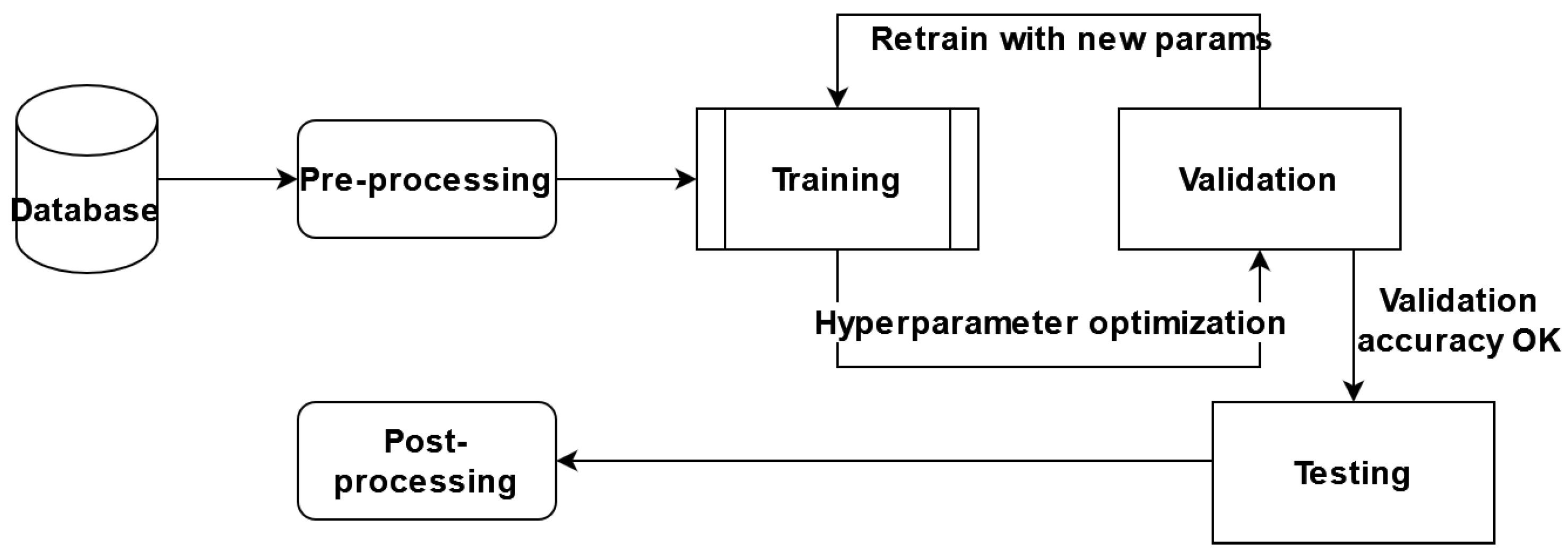
In this paper, we proposed performing certain experiments on the AWS Sagemaker platform and adapting the predefined architectures for segmentation, with brain tumor segmentation as our goal. We adapted and trained six different architectures, a variant of the hyperparameter optimized model, and an ensemble of the models obtained. The general component diagram of our system is shown in Figure 6.
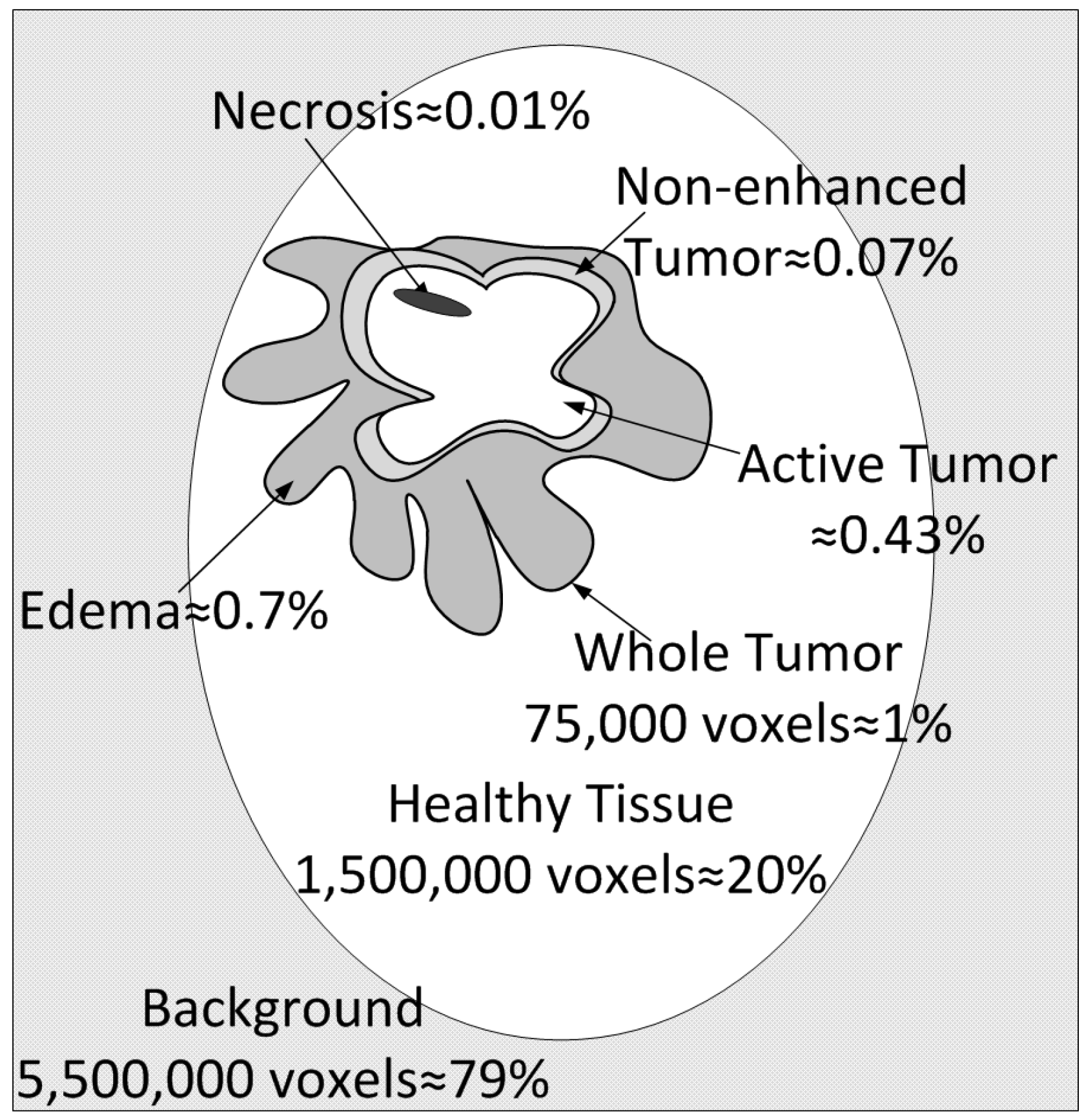
The database used for training is the publicly available BraTS 2017–2020 dataset. There are a total of 335 images, out of which 259 are glioblastoma (or high-grade tumor images) and 76 low-grade tumor MRI scans. Every image is 3D at a resolution of 240 × 240 × 155 pixels, and there are four image modalities in total (T1, T1c, T2 and Flair), plus the ground truth image labeled by multiple experts and included in the public dataset. Before the training process, we randomly split this dataset into training, validation, and test sets in a proportion of 60% (201 images), 20% (67 images), and 20% (67 images). Class imbalance exerts a highly undesirable influence on the training process. The most frequent pixels are learned the best; these constitute the background (78–79% of the total image voxels) and the healthy brain (20–21%). The least frequent by far are the tumor voxels, which represent a total of about 1% of the whole image. The different tumor types are edema (ED) at around 0.7%, non-enhanced tumor (NET) at 0.07%, active tumor (AT) at 0.43%, and necrosis (NEC) at 0.01% of the total number of voxels.
The implementation of the described algorithms was conducted via the Amazon SageMaker. The definition of classes on the input images uses consecutive class numbering from 0 to n (n = 5) in our case. There are however five classes because classes 2 and 4 are conjoined. Detection differentiates background and healthy regions much better than between different tumor tissues, which is caused by the mentioned class imbalance.
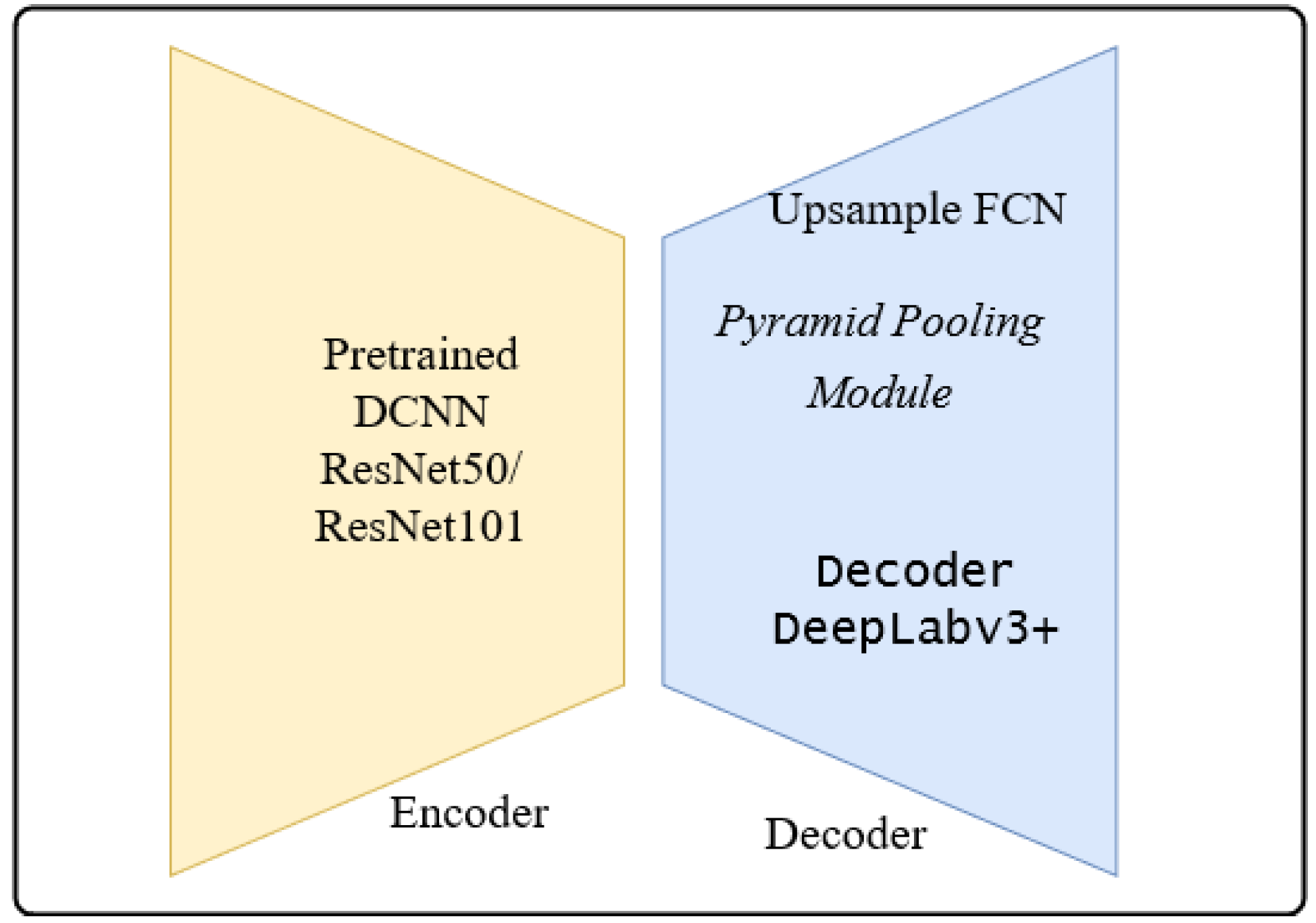
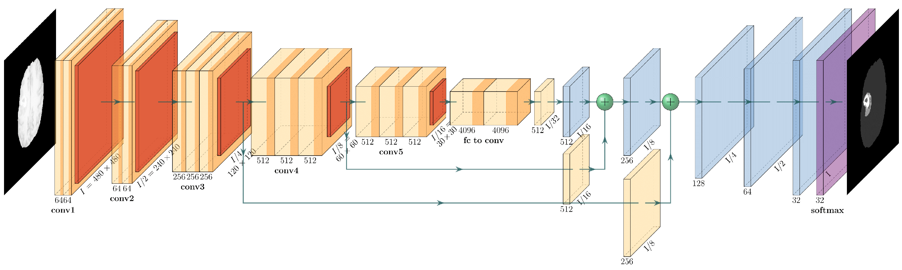
The architectures adapted to brain tumor segmentation follow the encoder-decoder architecture shown in Figure 7.
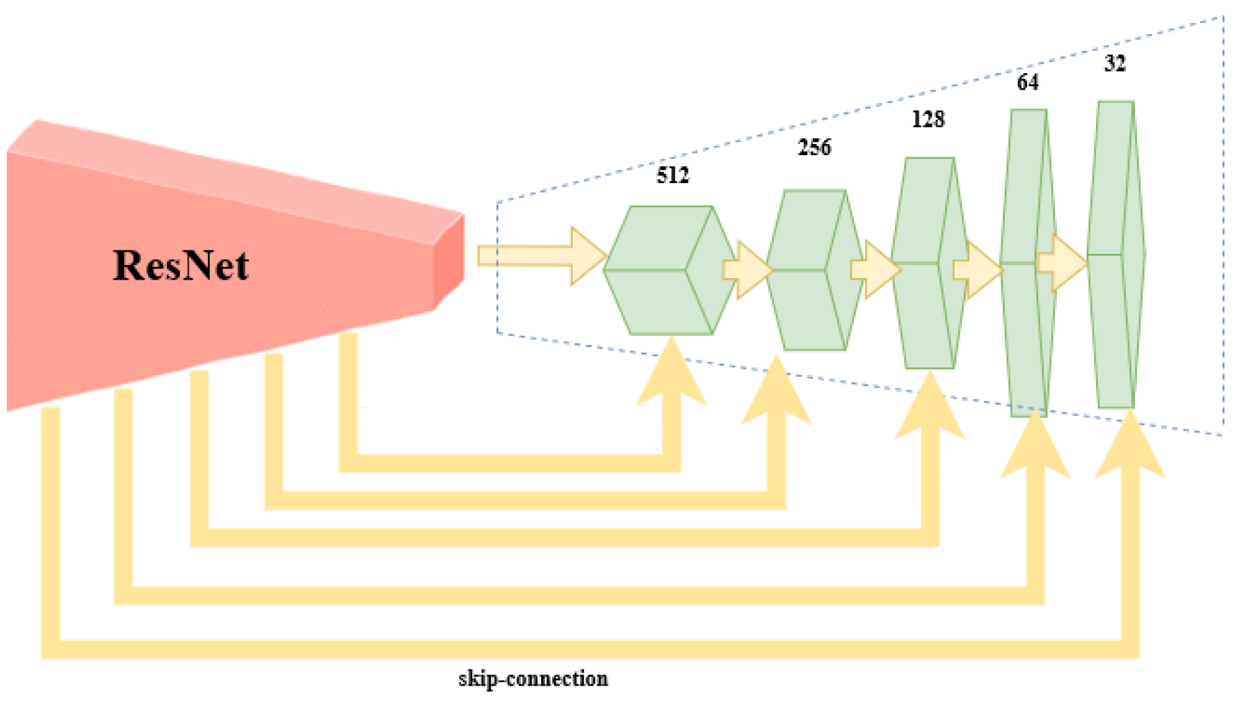
The encoder is the well-known ResNet50 or ResNet101 CNN initialized with pretrained weights of the ImageNet. The preloaded ImageNet weights can detect 1000 different objects from the ImageNet Challenge and are usually a good starting point for further training. The decoder is the up-sampling part of the smallest feature map obtained during encoding. The FCN up-sampling module is a three-layered upconvolution until the original dimension is reached again (
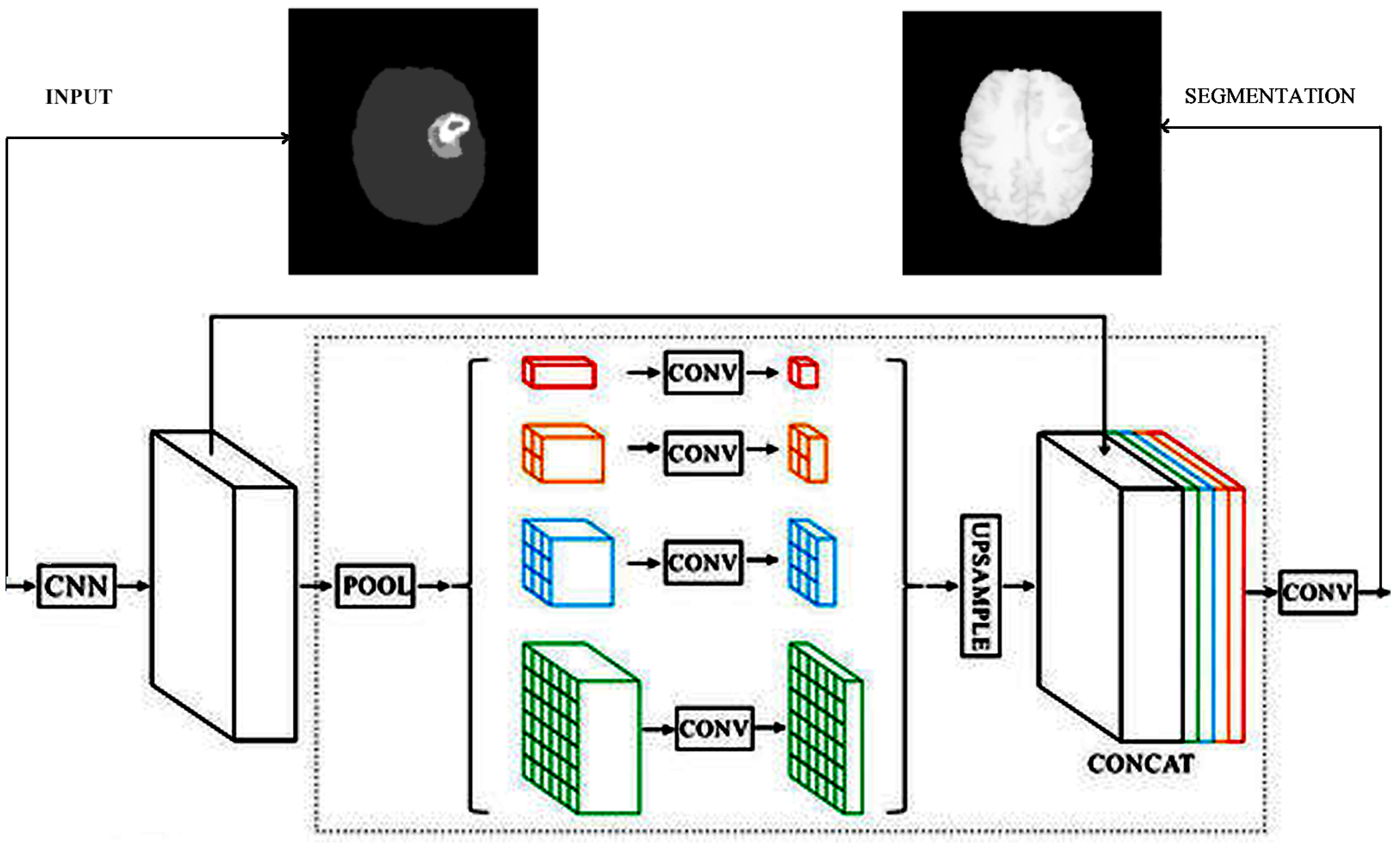
Figure 1). The next deconvolution architecture adapted for our task of brain tumor segmentation was the PSP architecture via the combination of feature maps of sub-blocks (
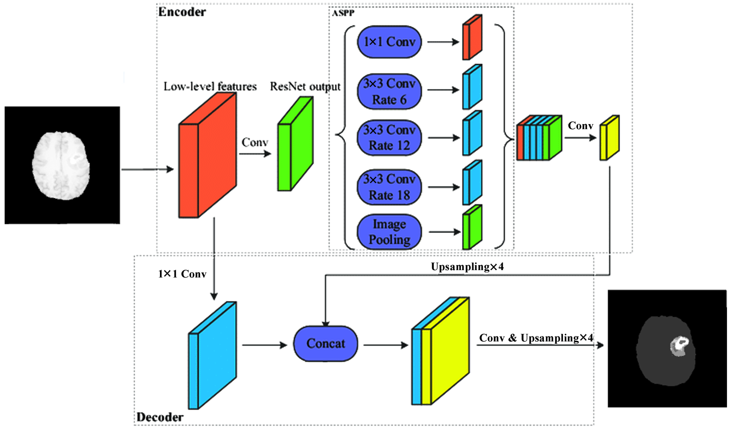
Figure 3). The third version of upconvolution is the DeepLab3+ decoder variant combining multi-scale feature maps by applying atrous convolution.
Using this method, six different CNN architectures were implemented and adapted for brain tumor segmentation. For all 6 architectures, the number of classes was 5, crop size was 240 × 240 pixels, the number of maximal epochs was 100, and the learning rate was 0.001. We used a polynomial learning rate scheduler with a scheduler factor of 0.1. The optimization method was SGD using a momentum value of 0.9 and an early stopping patience of four epochs. During the training process, we used the advantages of transfer learning. Transfer learning is a technique in machine learning that relies on knowledge obtained from one task applied to another task. Transfer learning in the case of CNNs can be used if the network architecture of the original and current networks is the same until a given layer. The weights to that point can be loaded from the CNN, trained in other purposes, into the current network. Thus, the training process starts considering those initial weights. In our case, the ImageNet weights were the initial weights. The ImageNet Challenge [51] differentiates 1000 usual objects, but has nothing to do with medical image segmentation. Due to applying the transfer learning technique, we were able to obtain better results with a smaller number of epochs than training the system without this technique. 
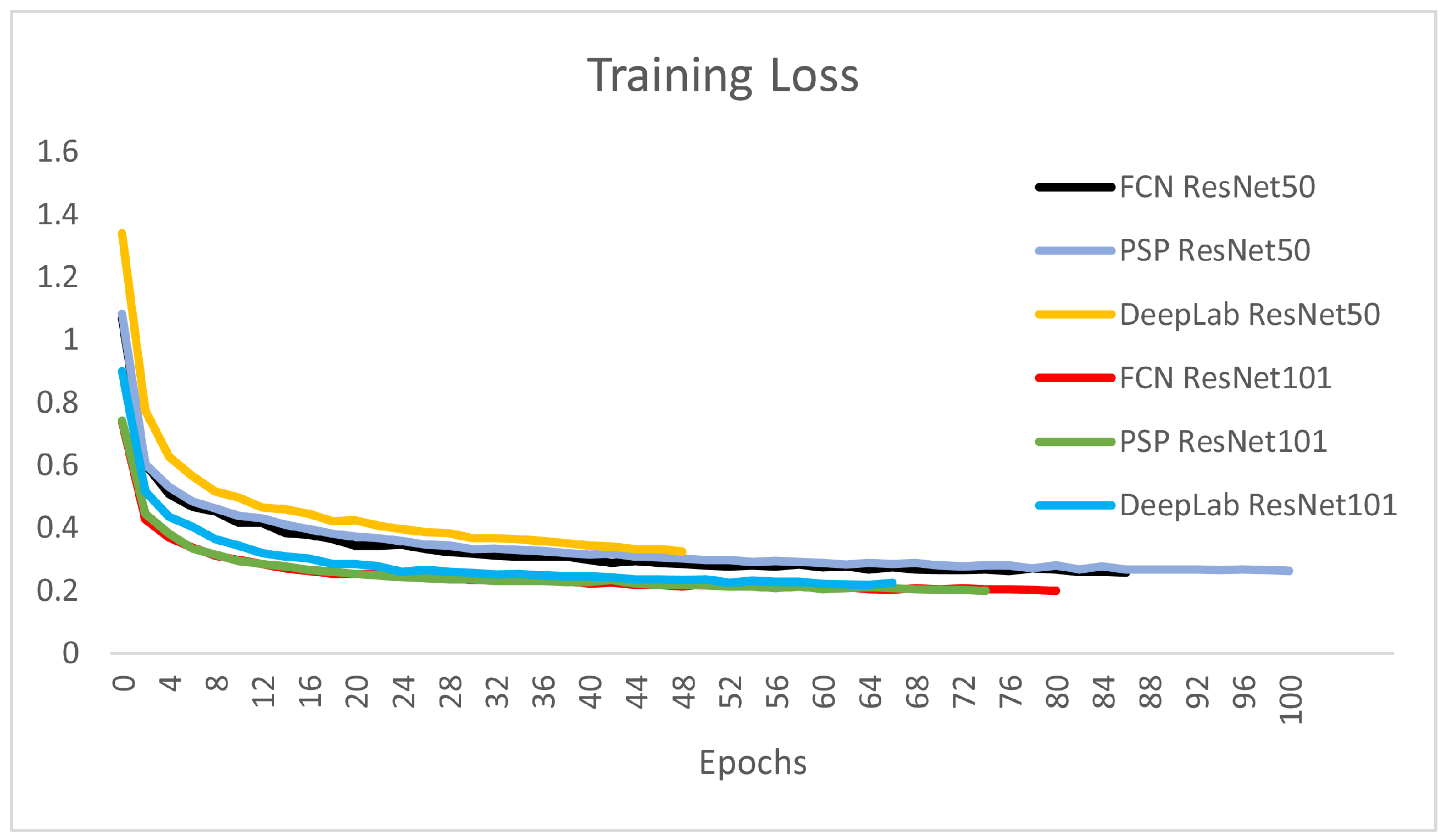
Figure 8 depicts the training loss over the progress of epochs for the six CNNs presented. It is obvious that the larger encoder architectures using ResNet101 are steeper and converge slightly faster in the training process.
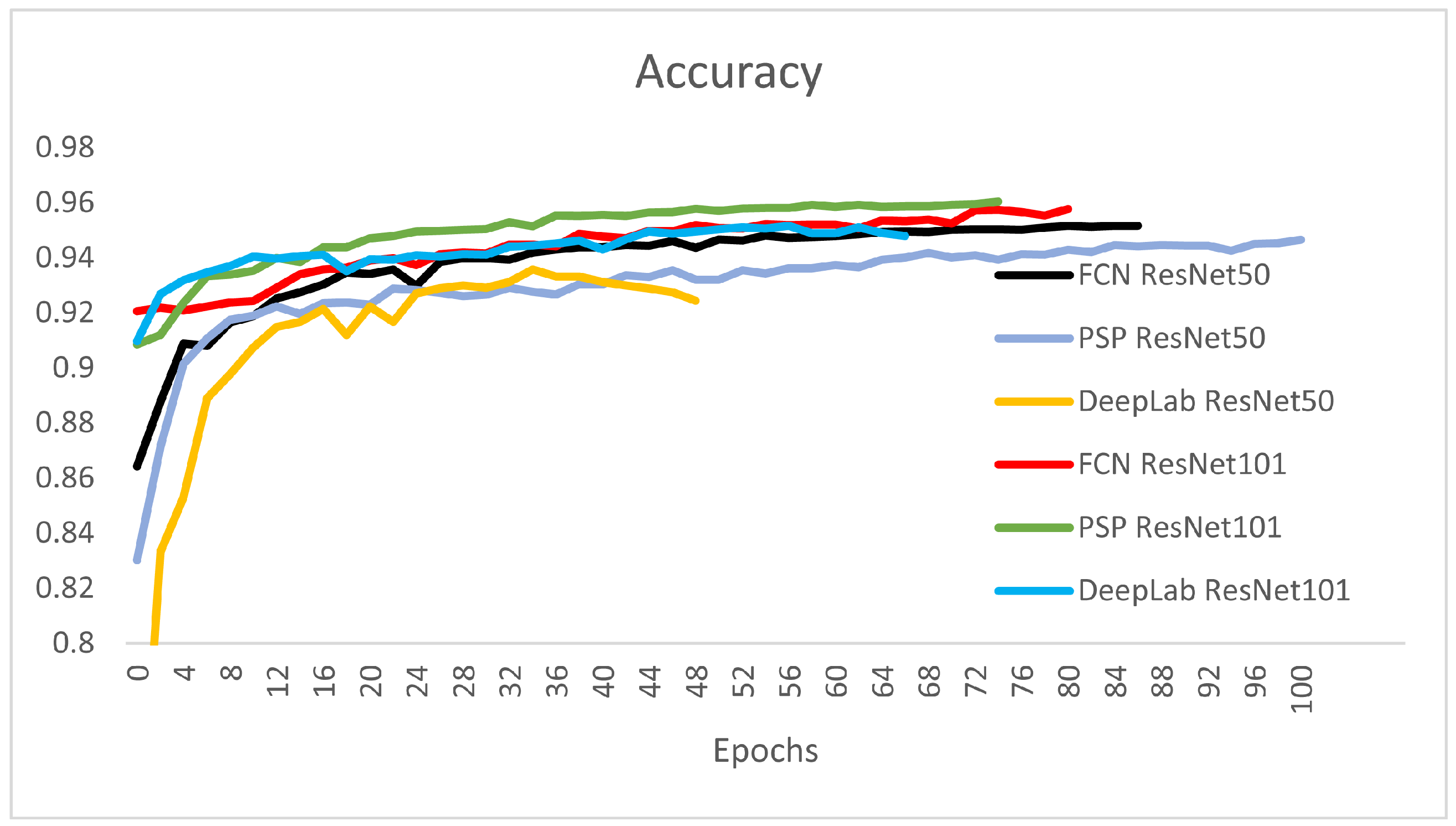
Figure 9 and Table 1 show the overall validation accuracy for the networks presented. From the perspective of the validation accuracy for all classes, the PSP-ResNet101 is the best, followed by FCN-ResNet101 and DeepLab-ResNet101. The overall validation accuracy is measured on the validation set and is obtained as the mean accuracy (Equation (2)) over all four classes.
A c c u r a c y = C o r r e c t p i x e l s i n p r e d i c t e d s e g m e n t a t i o n T o t a l p i x e l s i n s e g m e n t a t i o n ,
m e a n A c c u r a c y = 1 | C l a s s e s | c C l a s s e s C o r r e c t p i x e l s i n p r e d i c t e d s e g m e n t a t i o n o f c l a s s c T o t a l p i x e l s i n s e g m e n t a t i o n o f c l a s s c ,
It can be observed that the DeepLab-ResNet50 was stopped at epoch 49 because it had the highest training loss and lowest validation accuracy from all the six architectures.The best architecture from the perspective of overall accuracy are the DeepLab-ResNet101, PSP-ResNet101, FCN-ResNet101, and FCN-ResNet50. The stopping condition of the final epoch was set by considering the stopping patience of four epochs with non-decreasing training loss, and the stopping tolerance was set to 0.001. This was the reason for different stopping epochs of the networks (Table 1).
The quantitative evaluation of different architectures was conducted by computing the Dice score on the test set. The Sørensen–Dice score measures the similarity of two samples; in our case, the similarity between the ground truth (GT) and the segmentations obtained (predicted segmentations). It is twice the overlap area over the cardinality of both sets (Equation (3)). In the case of binary segmentation, it can be expressed by the 2 × TPR (true positive rate) over the total number of pixels: 2 × TPR + FPR (false positive rate) + FNR (false negative rate).
D i c e S c o r e = 2 × | P r e d G T | | P r e d | + | G T | = 2 × T P R 2 × T P R + F P R + F N R ,
In the case of multi-class classification, the Dice score is computed considering class i and class n o n i for all other pixels.
In the training process of the six different networks, we used the mIOU (Equation (9)) as the loss function of the optimization algorithm. The mean intersection over reunion is a region-based loss function, also called the Jaccard loss. The Jaccard loss and the Dice loss [52] are very similar losses, and they can be alternatively used in segmentation tasks.
J a c c a r d l o s s = 1 J a c c a r d = 1 D i c e s c o r e 2 D i c e s c o r e ,
D i c e l o s s = 1 D i c e = 1 2 × J a c c a r d 1 + J a c c a r d ,
The Tversky Distance [53] is a generalization of the Dice loss that considers the true positive pixels over a weighted sum of true positives and false positives and false negatives.
T v e r s k y l o s s = 1 T v e r s k y d i s t a n c e = 1 T P + ϵ T P + α × F P + β × F N + ϵ ,
We have considered this type of loss too, but it can improve the training loss if it is considered on binary segmentation cases. In our case, the coefficients weighting the FP and FN in the nominator have to be setup separately form one class to the other. This can be completed if the five-class segmentation is divided into four times applied binary segmentation (Background-Healthy; Healthy-Whole Tumor; Edema-Tumor Core; Enhanced Tumor-Necrosis/Non-Enhanced Tumor). This multiple binary classification pipeline will surely bring considerable improvement because the class imbalance is eliminated and, the loss is computed not based on a mean loss of all the classes, but considering the two relevant classes at each binary classification phase.
In Table 2, we measured the Dice scores for background voxels, healthy voxels, and the Whole Tumor (classes 2/4 + 3 + 5). The detection of background and healthy voxels is as expected. Background Dice is between 99.29 and 99.7%, and for healthy voxels, the Dice is between 95.99 and 97.46%. The detection of tumor voxels is about 90% (88.89–90.66%), which is a good result compared to the BraTS Challenge WT (Whole Tumor) average of 82.74%. The average WT Dice score of the BraTS Challenge is based on the validation table results, namely, the Validation Leaderboard [14]. The best result on the leaderboard had a Dice coefficient of 92.45%, and 80 participants out of a total of 291 are above 90%.
Table 3 shows the results of the six different architectures on the three types of tumor tissue: edema (ED), active tumor (AT), and necrotic and non-enhanced tumor (NEC/NET). Both the edema and active tumor were about 70%. The worst results of 38–47% were obtained on the NEC/NET tissue type. In Table 1 and Table 2, ResNet101 is slightly better than the ResNet50 architecture. The best results were obtained by DeepLab-ResNet101 for AT (73.7%) and NEC/NET (47.63%) and PSP-ResNet101 for ED (75.21%).
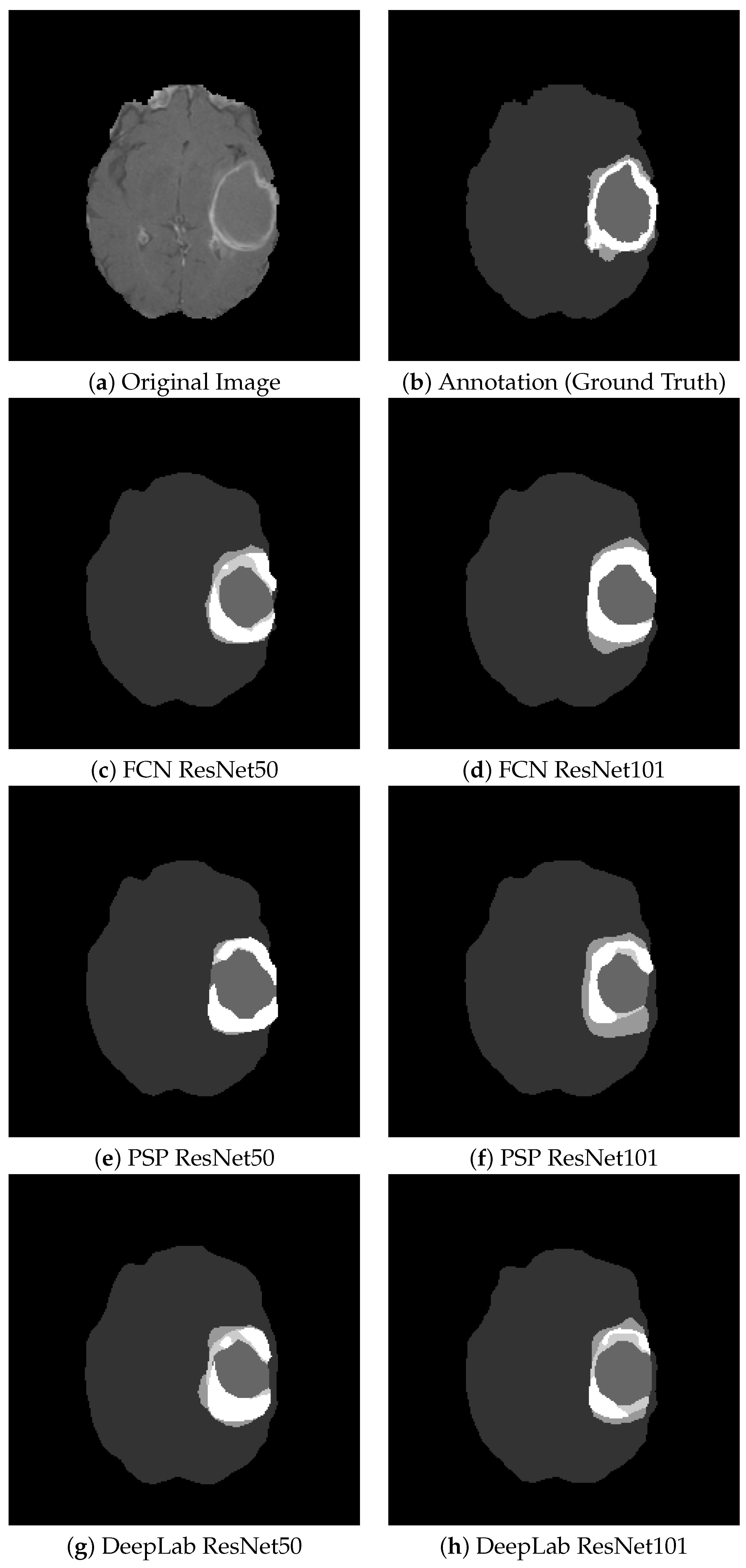
Figure 10 shows some segmentation results for the visual comparison of different tumor types and the six architectures studied. On average, this barely visible difference is around 1–2%. There is no quantitative evidence clearly showing that one architecture is better than all the others. In different images, the other architecture outstrips the rest. This led to the idea of combining them into an ensemble model.
The second group of experiments was related to hyperparameter optimization to possibly extract the best architecture from it.
The training jobs and hyperparameter optimization setup that had to be defined in the Amazon SageMaker framework were related to the six types of CNN networks, their hyperparameters, and the input database type. The data were provided in pipe mode stored in an S3-bucket. These data were accessed via an AugmentedManifestFile containing the path to every image and to every corresponding annotation file along with the training job name and other metadata. The validation and test data were provided in the same way. The hyperparameter tuning job was run on an ml.p3.2xlarge system on three instances. Every instance was set to run a maximum of five parallel training jobs. The maximum duration per training job was set to 48 h.
SageMaker hyperparameter tuning uses Grid Search and Bayesian Search [54] to obtain the best set of parameters. The tuning algorithm for SageMaker performs guesses as to which sets of hyperparameters are likely to achieve better results and runs the training jobs with those parameters.
The training job is abandoned before the preset number of epochs if another training job had better results regarding the objective metric in the same iteration. The objective metric was the mIOU (mean intersection over reunion). IOU computes the intersection over reunion between the predicted segmentation and the ground truth for every image (Equation (7)). The meanIOU computes the average value of IOU for every image (Equation (8)) over each class c C l a s s e s Equation (9).
I O U = | P r e d G T | | P r e d G T | ,
I O U I = 1 N i I | P r e d i G T i | | P r e d i G T i | ,
m I O U = 1 | C l a s s e s | c C l a s s e s I O U c I = 1 | C l a s s e s | · 1 N c C l a s s e s i I | P r e d i G T i | | P r e d i G T i | ,
This metric is the same as the Jaccard index (Equation (10)).The Jaccard index can be expressed not only by the IOU but also as a fraction of TPR over TPR + FPR + FNR.
J a c c a r d = | P r e d G T | | P r e d G T | = T P R T P R + F P R + F N R ,
The optimization parameters [55] that had to be set up to give reasonable and quite restricted intervals for them were the optimization function, learning rate, weight decay, momentum, and minibatch-size.
Firstly, we set the mini-batch size between 16 and 64. The optimization functions added in the optimization process were MB-SGD, SGD with momentum, AdaDelta, and Adagrad. SGD for mini-batches takes the gradient step for a mini-batch with a regularization term called weight decay (=0.0001) multiplied by the weight and added to the gradient. SGD with momentum reduces the fluctuation towards the optimal value by adding the momentum term. AdaGrad (Adapted Gradient Descent) modifies the learning rate in each iteration biased towards the past gradient of that parameter. Instead of the past gradient in AdaGrad, AdaDelta modifies the learning rate by the average over the past squared gradients of a weight.
The learning rate scheduler controls the decrease in the initial learning rate over time over the progress of the epochs. The learning rate is multiplied by a factor of 0.1 after a given number of epochs (=10). The early stopping algorithm stops a training job if certain stopping conditions are met. The minimum number of epochs was set to 5, early stopping patience was 4, and early stopping tolerance was 0.001.
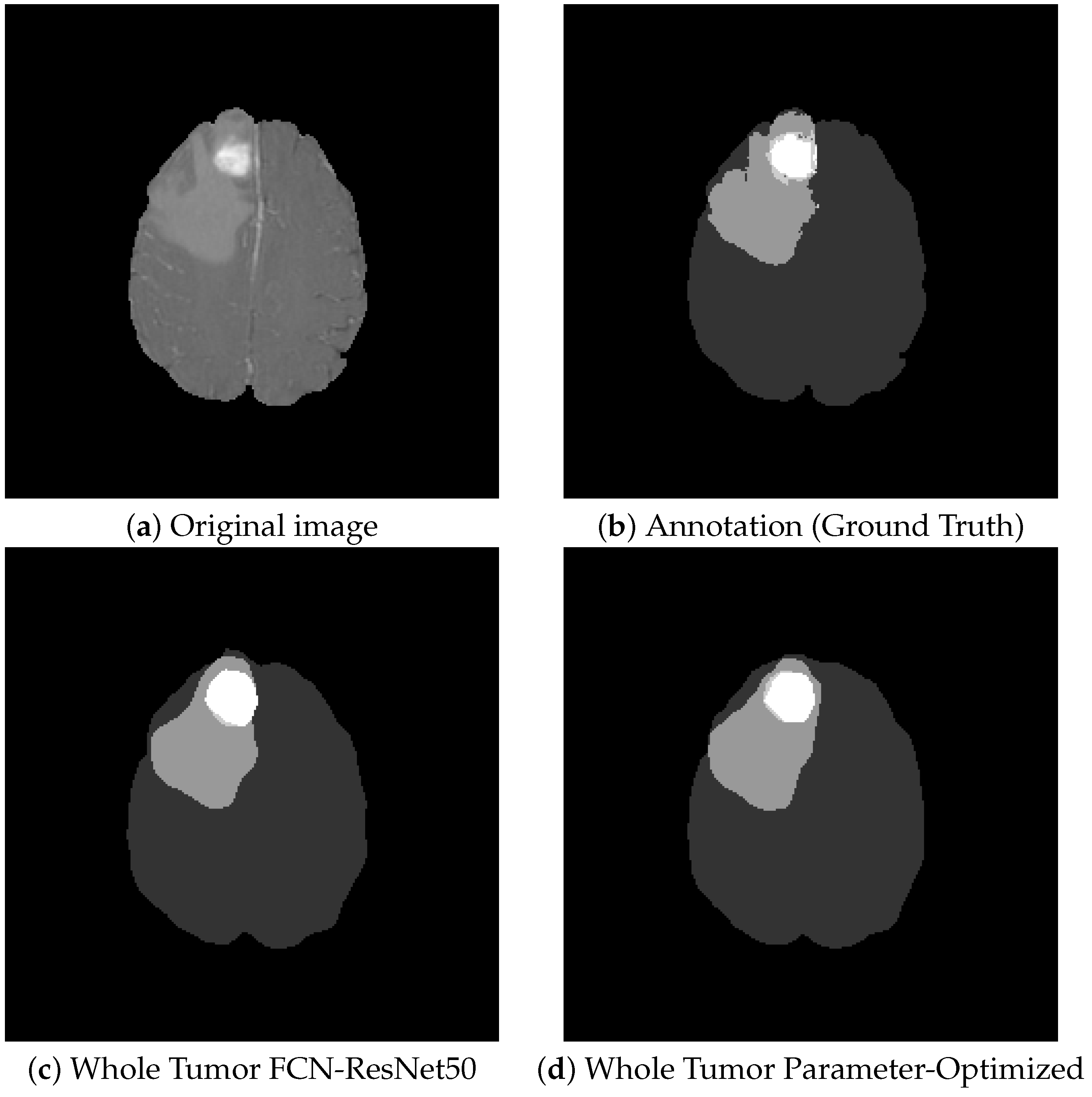
Hyperparameter optimization was conducted for only one architecture of the six studied, namely, FCN-ResNet50. The best parameters obtained via hyperparameter optimization were minibatch-size = 18, learning rate = 0.0009, weight decay = 0.0114, momentum = 0.803, and the AdaGrad optimization method. Several training jobs with different parameter setups stopped before the end of the job, recognizing at a very early epoch that their process involving the optimization metric is smaller than the best thus far. The validation mIOU for the best hyperparameter setup was 0.7732. This mIOU is a value similar to the one obtained for the first variant of FCN-ResNet50 without hyperparameter optimization (mIOU = 0.7649).
We note that the hyperparameter optimization procedure provided by the SageMaker framework did not lead to considerably better results for the following reasons: 42 different parameter sets were tried, and out of these, only about 10 ran until the end, namely, 100 epochs, for about 48 h per training job of the 10 runs (200 h in total). In these 42 jobs, the batch size, learning rate, weight-decay, and momentum parameters were selected according to a random grid search. Out of the optimization functions, only AdaGrad and SGD were selected. The Sagemaker hyperparameter optimization process slightly modified the numerical parameters for each run of a different training job. The only parameter that was modified considerably on a logarithmic scale was the learning rate. The enormous resource requirements coupled with the small improvement achieved made us decide against running the hyperparameter optimization on the five other architectures studied.
From Table 4 and Table 5, we can see that the FCN with parameter optimization led to a barely observable Dice score improvement of 0.8% on average for all classes.
Figure 11 shows a visual comparison of tumor tissue segmentation with and without hyperparameter optimization on the FCN-ResNet50 architecture. On average, there is an improvement of only about 1% to the detriment of the enormous computational complexity.
The last group of experiments that were carried out was related to the combination of all six segmentation models in an attempt to obtain a so-called ensemble model from them. We obtained weighted segmentation maps from all six individual classifiers presented above.
Comparing Table 2, Table 4, and Table 6, we can draw the following conclusions: The Dice score for the Whole Tumor is reduced by approximately 2–3% compared to the best method out of the six. On the other hand, the Dice scores for different tumor tissues of the ensemble model are better by about 4–10% (Table 3, Table 5 and Table 7). This is a considerable improvement.
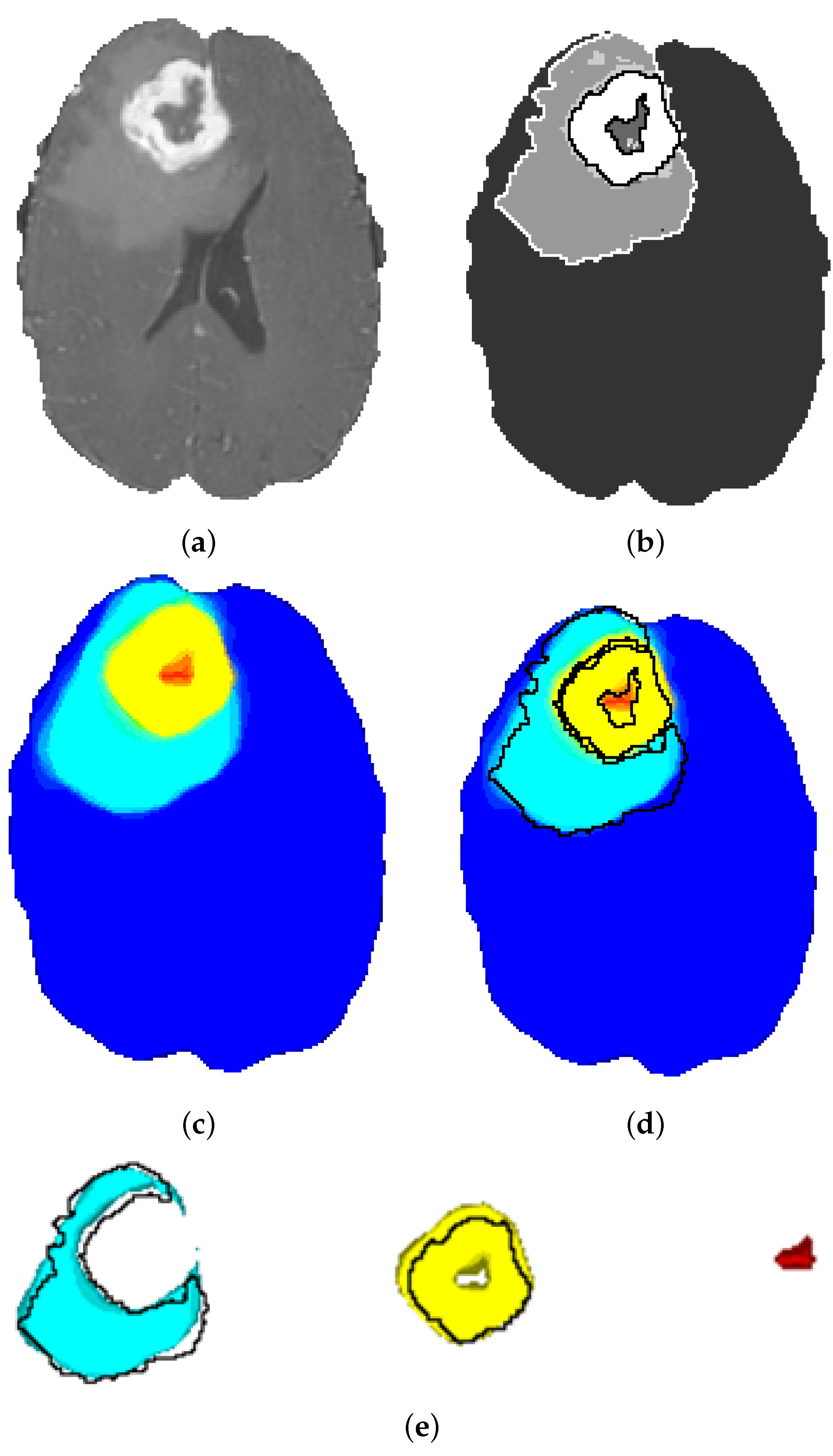
The segmentation maps obtained by the ensemble model are depicted in Figure 12. It is obvious that the tissue contours and transitions from one tissue to the other are gradually colored from turquoise to yellow, and there is a slight green ring at the transition. This shows that the ensemble model obtains a probability map and does not make a final decision favoring any class for uncertain tissue voxels on the contour. These voxels are, in fact, the hard examples and are not clearly classifiable. The probabilistic heatmap of the ensemble model solves this problem through probabilistic voting.
Overall, we propose the sequential application of the best DeepLabv3 model or the parameter-optimized FCN ResNet50 for obtaining the tumoral region, and after that, finetuning the results by obtaining the different tumor tissues through the use of the ensemble model. Finally, to highlight our results, we compare them to the best results from the BraTS Challenge 2020, published in 2021.
All our experiments were conducted on the p3.2xlarge AWS EC2 instance. That is a Tesla V100 GPU with 16 GB memory. By running only on Spot instances instead of on-demand usage, we could carry out our experiments on a very low cost of USD 200–300.
The most important advantage of our model is the relatively low number of epochs (80–100) each CNN is trained for. Overall, the training process lasted under 12 h for each of the presented models (Table 8). The more complex networks that achieve better results have to be trained much more, even 4–5 days on multiple GPUs with larger computational capacity and memory [39].
As can be seen, our results are comparable with the competition performances between 2017 and 2020. Our goal with this article was to create simple models available in the AWS Sagemaker that can be easily combined into an ensemble model with good performances. The Dice score of the tumor core is 0.8599 for our ensemble model, which is comparable to the best results. The goal in our research was not to obtain the best results but to create a rapidly trainable system that can be applied for other types of medical image segmentation in a similar way. The performances of such a system can be considered quite competitive. The Dice score differences of 1–5% out of the tumor tissue volume of every type comes from the slightly inaccurate contour detection. A contour delimitation displaced with a single voxel considerably influences the Dice score results, especially on small tumors of a few voxels. The exact contours are always re-evaluated by the neurosurgeons during preoperative planning before a gross-total resection.

4. Discussion

In the BraTS Challenge, the tumor tissue types are grouped into different tumor regions. The NEC/NET results are not considered separately. The Leaderboard results show the Enhancing Tumor (ET = class 5), the Whole Tumor (WT = classes 2/4 + 3 + 5), and Tumor Core (2/4 + 5 = NEC/NET + AT). The Leaderboard of the BraTS competition shows the results of the various participating teams, measuring the Dice scores on the so-called validation dataset. At the BraTS 2020 competition, there were 292 teams present on the Leaderboard.
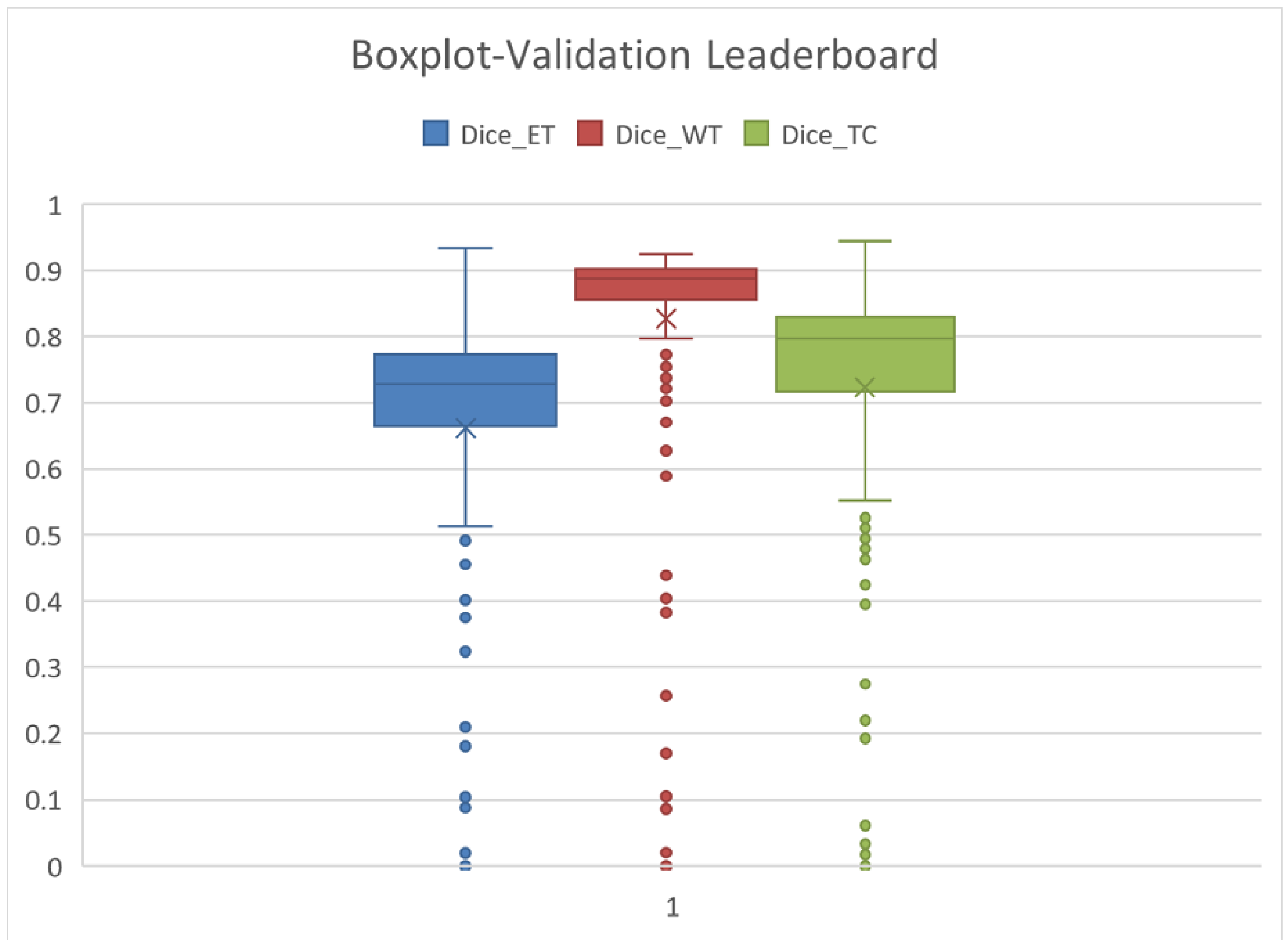
The statistics related to the average results are detailed in Table 9 and Figure 13. The average is marked by X, the median is the center-line, and the Q1 and Q3 values are the lower and upper margins of the box.
The mean and Q3–75% quartiles are relevant from our perspective. Our results regarding ET, WT, and TC, as presented in Table 10, are far better than the average of the Leaderboard and are comparable to the Q3 quartile results. This means that our results are among the first 25% of the Leaderboard.
We compare our results obtained on the test set, which is 20% taken separately from the BraTS dataset. The Leaderboard results are measured on a validation dataset not publicly available. If we consider both datasets being sufficiently general, the results are comparable.
Table 10 presents our results from the six different architectures and the BraTS tumor regions. The three tumor regions are ET (Enhanced Tumor), Whole Tumor (WT), and TC (Tumor Core). The best Dice scores we obtained are about 90% for WT, 84% for TC, and 78% for ET.
The best results obtained in the BraTS competition are presented in Table 11. These are slightly worse than the Leaderboard maximums. The competition score is a result of a one-time experiment, making the progressive architecture adjustments impossible, whereas the leaderboard score is the best score achieved by a team. Therefore, the best results at competitions are 7–8% worse than the best results on the leaderboard.
Comparing the six different architectures (Table 9) with the ensemble model, we can see a 2% decrease in the Dice score for WT but a 2% increase for ET and TC (Table 12).
Overall, we obtained fairly good results that are comparable to the BraTS Leaderboard results. We suggest applying the best model for WT (DeepLab-ResNet101), and after that, finetuning the contour regions between different tumor tissues with the ensemble model.
However, our results are quite competitive, and they will be improved in several ways. We propose some aspects for future improvement and further development.
The quality and resolution of the images is not standardized. In the image augmentation stage, we normalize the images to a mean of 0 and a standard deviation of 1, but the inhomogeneity correction should also be applied before the training process.
Better results could be obtained if the five-class classification process were divided into four binary classification steps. First, the tumor should be delimited from the background (including healthy tissue). Next, the tumor types should be discovered according to the anatomical structure depicted in Figure 5. Accordingly, the edema can be delimited next, followed by the tumor core, and the very last should be the delimitation of the necrotic tumor. This type of structure may be also discovered by wearing AR-based neuronavigators that have a crucial importance in preoperative planning and a simulation of surgical scenario [56,57]. Considering multiple binary classification steps and not a single five-class classification, the tumor types with a considerably smaller number of representative voxels in the database would be much better delimited. This issue can be eliminated through the random sampling of the initial images at a smaller given patch size, with the goal of including the same number of healthy and tumoral tissue pixels in the database. The most important bottleneck of the models obtained is the slightly inaccurate contour detection. The cause of these less-precise boundary detections is the multi-class classification and the class imbalance. This can be further corrected by introducing different architectures specifically trained for boundary detection.
As a post-processing step, we propose the verification of tumor structure connectedness. The tumor is a connected region without any holes or gaps. In addition, the anatomical structure of the tumor can be a posterior condition, knowing that some tissues should be inside others: necrotic tumor ⊆ tumor core ⊆ edema. The improvements suggested should furthermore improve the results obtained thus far.
The ensemble model based on the combined response of the six CNNs has similar results for the tumor core as the results presented in the BraTS Challenge (Table 11 and Table 12).

5. Conclusions

The results and experiments presented above describe an automatic brain tumor segmentation approach based on the tools in AWS Sagemaker for building CNN networks and hyperparameter optimization techniques. In our results, we compare three different architectures: FCN, PSP, and DeepLab encoder-decoder networks, each with two encoder versions (ResNet50 and ResNet101). For the encoder part, we loaded in the ImageNet weights to use transfer learning. The encoders were subsequently trained, and the decoders were trained from the beginning. In our paper, we fine-tuned the hyperparameters and applied the advantages of transfer learning to obtain segmentation results on the BraTS database with the purpose of brain tumor segmentation. The system can be a very helpful tool for physicians and neurosurgeons. Brain MRI examination and a possible introduction of a regular MRI screening once every 2 years on the whole population or on the risk-patients is becoming widespread. This automated system can give an 80–90% exact segmentation response and can indicate to patients who really have suspicious cells on their MRI record to consult a doctor. The tumor can be detected even in an incipient phase, preventing HGG tumors if possible. This type of frequent examination would discover the LGG tumors in initial phases. The results obtained are comparable to the BraTS Challenge Leaderboard results and are among the first quartile in ranking. The best Dice scores we have obtained for WT are about 90%, TC 84%, and ET 78%.
The purpose of this research was to create an end-to-end system suitable for multi-modal brain tumor segmentation that is able to differentiate the whole tumor, tumor core, healthy tissue, and background. We have adapted six different convolutional neural networks known in the literature. In our experiments, we demonstrated that these simple architectures with few parameters and a good hyperparameter setup can achieve similar results to the best ones competing in BraTS Challenges. In these architectures, the transfer learning techniques were used, and in this way, the CNNs have been trained with much fewer epochs. The training and testing phases could be conducted in less time with a smaller budget. This permits retaining and fine-tuning the current performances to include different MRI multi-modal brain datasets acquired over time in clinical environments.

Author Contributions

Conceptualization, S.L. and L.L.; methodology, S.L. and L.L.; software, S.L.; validation, S.L. and L.L.; formal analysis, L.S.; investigation, S.L.; resources, S.L. and L.L.; data curation, L.L.; writing—original draft preparation, S.L.; writing—review and editing, S.L., L.L. and L.S.; visualization, L.L.; supervision, L.L. and L.S.; project administration, S.L.; funding acquisition, S.L. All authors have read and agreed to the published version of the manuscript.

Funding

The work was supported by the University of Medicine, Pharmacy, Science, and Technology “George Emil Palade” of Târgu Mureș, Research Grant Number 292/4/14.01.2020.

Institutional Review Board Statement

Not applicable.

Informed Consent Statement

Not applicable.

Data Availability Statement

The brain MRI records processed in this study are available at the BraTS website: https://www.med.upenn.edu/cbica/brats2021/ accessed on 27 February 2022.

Conflicts of Interest

The authors declare no conflict of interest.

Abbreviations

The following abbreviations are used in this manuscript:
AIArtificial Intelligence
ATActive Tumor
BraTSBrain Tumor Segmentation Challenge
CNNConvolutional Neural Network
CTComputed Tomography
DCNNDeep Convolutional Neural Network
EDEdema
ETEnhanced Tumor
FCNFully Convolutional Network
FPRFalse Positive Rate
FNRFalse Negative Rate
GBMGlioblastoma Multiforme
GTGround Truth
HGGHigh-grade Glioma
IOUIntersection over Reunion
LGGLow-grade Glioma
MB-SGDmini-batch Stochastic Gradient Descent
MRIMagnetic Resonance Imaging
mIOUmean Intersection over Reunion
NECNecrosis
NETNon-Enhanced Tumor
PETPositron Emission Tomography
PredPrediction
PSPNetPyramid Scene Parsing Network
ResNetResidual Network
SGDStochastic Gradient Descent
SPECTSingle-Photon Emission Computerized Tomography
T1longitudinal relaxation time
T1GdT1 Gadolinium contrast media
T1clongitudinal relaxation time with contrast
T2transverse relaxation time
T2-FLART2-weighted-Fluid-Attenuated Inversion Recovery
TCTumor Core
TCGAThe Cancer Genome Atlas
TPRTrue Positive Rate
TNRTue Negative Rate
WHOWorld Health Organization
WTWhole Tumor

References

  1. Louis, D.N.; Perry, A.; Wesseling, P.; Brat, D.J.; Cree, I.A.; Figarella-Branger, D.; Hawkins, C.; Ng, H.K.; Pfister, S.M.; Reifenberger, G.; et al. The 2021 WHO Classification of Tumors of the Central Nervous System: A summary. Neuro-Oncology 2021, 23, 1231–1251. [Google Scholar] [CrossRef] [PubMed]
  2. Sang-Geun Choi, C.B.S. Detection of HGG and LGG Brain Tumors using U-Net. Med. Leg. Update 2019, 19, 560–565. [Google Scholar] [CrossRef]
  3. Montemurro, N.; Fanelli, G.; Scatena, C.; Ortenzi, V.; Pasqualetti, F.; Mazzanti, C.; Morganti, R.; Paiar, F.; Naccarato, A.; Perrini, P. Surgical outcome and molecular pattern characterization of recurrent glioblastoma multiforme: A single-center retrospective series. Clin. Neurol. Neurosurg. 2021, 207, 106735. [Google Scholar] [CrossRef] [PubMed]
  4. Menze, B.H.; Jakab, A.; Bauer, S.; Kalpathy-Cramer, J.; Farahani, K.; Kirby, J.; Burren, Y.; Porz, N.; Slotboom, J.; Wiest, R.; et al. The Multimodal Brain Tumor Image Segmentation Benchmark (BRATS). IEEE Trans. Med. Imaging 2015, 34, 1993–2024. [Google Scholar] [CrossRef]
  5. Bakas, S.; Akbari, H.; Sotiras, A.; Bilello, M.; Rozycki, M.; Kirby, J.; Freymann, J.; Farahani, K.; Davatzikos, C. Advancing the Cancer Genome Atlas glioma MRI collections with expert segmentation labels and radiomic features. Sci. Data 2017, 4, 170117. [Google Scholar] [CrossRef] [Green Version]
  6. Baid, U.; Ghodasara, S.; Bilello, M.; Mohan, S.; Calabrese, E.; Colak, E.; Farahani, K.; Kalpathy-Cramer, J.; Kitamura, F.C.; Pati, S.; et al. The RSNA-ASNR-MICCAI BraTS 2021 Benchmark on Brain Tumor Segmentation and Radiogenomic Classification. arXiv 2021, arXiv:2107.02314. [Google Scholar]
  7. Gordillo, N.; Montseny, E.; Sobrevilla, P. State of the art survey on MRI brain tumor segmentation. Magn. Reson. Imaging 2013, 31, 1426–1438. [Google Scholar] [CrossRef]
  8. Breiman, L. Random Forests. Mach. Learn. 2001, 45, 5–32. [Google Scholar] [CrossRef] [Green Version]
  9. Lefkovits, L.; Lefkovits, S.; Szilágyi, L. Brain tumor segmentation with optimized random forest. In International Workshop on Brainlesion: Glioma, Multiple Sclerosis, Stroke and Traumatic Brain Injuries; Springer: Berlin/Heidelberg, Germany, 2016; pp. 88–99. [Google Scholar] [CrossRef]
  10. Gyorfi, A.; Szilágyi, L.; Kovács, L. A Fully Automatic Procedure for Brain Tumor Segmentation from Multi-Spectral MRI Records Using Ensemble Learning and Atlas-Based Data Enhancement. Appl. Sci. 2021, 11, 564. [Google Scholar] [CrossRef]
  11. Ronneberger, O.; Fischer, P.; Brox, T. U-Net: Convolutional Networks for Biomedical Image Segmentation. arXiv 2015, arXiv:1505.04597. [Google Scholar]
  12. Milletari, F.; Navab, N.; Ahmadi, S. V-Net: Fully Convolutional Neural Networks for Volumetric Medical Image Segmentation. In Proceedings of the 2016 Fourth International Conference on 3D Vision (3DV), Stanford, CA, USA, 25–28 October 2016; IEEE Computer Society: Los Alamitos, CA, USA, 2016; pp. 565–571. [Google Scholar] [CrossRef] [Green Version]
  13. Çiçek, Ö.; Abdulkadir, A.; Lienkamp, S.S.; Brox, T.; Ronneberger, O. 3D U-Net: Learning Dense Volumetric Segmentation from Sparse Annotation. In Medical Image Computing and Computer-Assisted Intervention—MICCAI 2016; Springer International Publishing: Berlin/Heidelberg, Germany, 2016; pp. 424–432. [Google Scholar] [CrossRef] [Green Version]
  14. Brain Tumor Segmentation (BraTS) Challenge. 2021. Available online: https://www.med.upenn.edu/cbica/brats2021/ (accessed on 27 February 2022).
  15. Liu, Z.; Chen, L.; Tong, L.; Zhou, F.; Jiang, Z.; Zhang, Q.; Shan, C.; Wang, Y.; Zhang, X.; Li, L.; et al. Deep Learning Based Brain Tumor Segmentation: A Survey. arXiv 2020, arXiv:2007.09479. [Google Scholar]
  16. Zikic, D.; Ioannou, Y.; Criminisi, A.; Brown, M. Segmentation of Brain Tumor Tissues with Convolutional Neural Networks. Proc. MICCAI-BRATS 2014, 36, 36–39. [Google Scholar]
  17. Jungo, A.; McKinley, R.; Meier, R.; Knecht, U.; Vera, L.; Pérez-Beteta, J.; Molina-García, D.; Pérez-García, V.M.; Wiest, R.; Reyes, M. Towards Uncertainty-Assisted Brain Tumor Segmentation and Survival Prediction. In Brainlesion: Glioma, Multiple Sclerosis, Stroke and Traumatic Brain Injuries; Springer International Publishing: Berlin/Heidelberg, Germany, 2018; pp. 474–485. [Google Scholar] [CrossRef]
  18. Kamnitsas, K.; Baumgartner, C.; Ledig, C.; Newcombe, V.F.J.; Simpson, J.P.; Kane, A.D.; Menon, D.K.; Nori, A.; Criminisi, A.; Rueckert, D.; et al. Unsupervised domain adaptation in brain lesion segmentation with adversarial networks. In International Conference on Information Processing in Medical Imaging; Springer: Cham, Switzerland, 2016. [Google Scholar]
  19. Castillo, L.S.; Daza, L.A.; Rivera, L.C.; Arbeláez, P. Brain Tumor Segmentation and Parsing on MRIs Using Multiresolution Neural Networks. In Brainlesion: Glioma, Multiple Sclerosis, Stroke and Traumatic Brain Injuries; Springer International Publishing: Berlin/Heidelberg, Germany, 2018; pp. 332–343. [Google Scholar] [CrossRef]
  20. Shen, H.; Wang, R.; Zhang, J.; McKenna, S.J. Boundary-Aware Fully Convolutional Network for Brain Tumor Segmentation. In Lecture Notes in Computer Science; Springer International Publishing: Berlin/Heidelberg, Germany, 2017; pp. 433–441. [Google Scholar] [CrossRef] [Green Version]
  21. McKinley, R.; Jungo, A.; Wiest, R.; Reyes, M. Pooling-Free Fully Convolutional Networks with Dense Skip Connections for Semantic Segmentation, with Application to Brain Tumor Segmentation. In Brainlesion: Glioma, Multiple Sclerosis, Stroke and Traumatic Brain Injuries; Springer International Publishing: Berlin/Heidelberg, Germany, 2018; pp. 169–177. [Google Scholar] [CrossRef]
  22. Byeon, W.; Breuel, T.M.; Raue, F.; Liwicki, M. Scene labeling with LSTM recurrent neural networks. In Proceedings of the 2015 IEEE Conference on Computer Vision and Pattern Recognition (CVPR), Boston, MA, USA, 7–12 June 2015. [Google Scholar] [CrossRef]
  23. Andermatt, S.; Pezold, S.; Cattin, P.C. Automated Segmentation of Multiple Sclerosis Lesions Using Multi-dimensional Gated Recurrent Units. In Brainlesion: Glioma, Multiple Sclerosis, Stroke and Traumatic Brain Injuries; Springer International Publishing: Berlin/Heidelberg, Germany, 2018; pp. 31–42. [Google Scholar] [CrossRef]
  24. Zheng, S.; Jayasumana, S.; Romera-Paredes, B.; Vineet, V.; Su, Z.; Du, D.; Huang, C.; Torr, P.H.S. Conditional Random Fields as Recurrent Neural Networks. In Proceedings of the 2015 IEEE International Conference on Computer Vision (ICCV), Santiago, Chile, 7–13 December 2015. [Google Scholar] [CrossRef] [Green Version]
  25. Kamnitsas, K.; Ledig, C.; Newcombe, V.F.; Simpson, J.P.; Kane, A.D.; Menon, D.K.; Rueckert, D.; Glocker, B. Efficient multi-scale 3D CNN with fully connected CRF for accurate brain lesion segmentation. Med. Image Anal. 2017, 36, 61–78. [Google Scholar] [CrossRef] [PubMed]
  26. Xue, Y.; Xu, T.; Zhang, H.; Long, L.R.; Huang, X. SegAN: Adversarial Network with Multi-scale L1 Loss for Medical Image Segmentation. Neuroinformatics 2018, 16, 383–392. [Google Scholar] [CrossRef] [Green Version]
  27. Bauer, S.; Wiest, R.; Nolte, L.P.; Reyes, M. A survey of MRI-based medical image analysis for brain tumor studies. Phys. Med. Biol. 2013, 58, R97. [Google Scholar] [CrossRef] [Green Version]
  28. Zikic, D.; Glocker, B.; Konukoglu, E.; Criminisi, A.; Demiralp, C.; Shotton, J.; Thomas, O.M.; Das, T.; Jena, R.; Price, S.J. Decision forests for tissue-specific segmentation of high-grade gliomas in multi-channel MR. In International Conference on Medical Image Computing and Computer-Assisted Intervention; Springer: Berlin/Heidelberg, Germany, 2012; pp. 369–376. [Google Scholar]
  29. Tustison, N.; Johnson, H.; Rohlfing, T.; Klein, A.; Ghosh, S.; Ibanez, L.; Avants, B. Instrumentation bias in the use and evaluation of scientific software: Recommendations for reproducible practices in the computational sciences. Front. Neurosci. 2013, 7, 162. [Google Scholar] [CrossRef] [Green Version]
  30. Dvorak, P.; Menze, B. Local Structure Prediction with Convolutional Neural Networks for Multimodal Brain Tumor Segmentation. In International Conference on Medical Image Computing and Computer-Assisted Intervention; Springer: Cham, Switzerland, 2016; Volume 9601, pp. 59–71. [Google Scholar] [CrossRef]
  31. Maier, O.; Wilms, M.; Handels, H. Highly discriminative features for glioma segmentation in MR volumes with random forests. In Proceedings of the Multimodal Brain Tumor Image Segmentation Challenge (MICCAI-BRATS); 2015; pp. 38–41. Available online: https://scholar.google.com.sg/scholar?hl=en&as_sdt=0%2C5&q=Highly+discriminative+features+for+glioma+segmentation+in+MR+volumes+with+random+forests&btnG=#d=gs_cit&u=%2Fscholar%3Fq%3Dinfo%3AIECXgD0TU0sJ%3Ascholar.google.com%2F%26output%3Dcite%26scirp%3D0%26hl%3Den (accessed on 27 February 2022).
  32. Chang, P.D. Fully Convolutional Neural Networks with Hyperlocal Features for Brain Tumor Segmentation. In International Conference on Medical Image Computing and Computer-Assisted Intervention; Springer: Berlin/Heidelberg, Germany, 2016; pp. 4–12. [Google Scholar]
  33. Myronenko, A. 3D MRI brain tumor segmentation using autoencoder regularization. In International MICCAI Brainlesion Workshop; Springer: Berlin/Heidelberg, Germany, 2018; pp. 311–320. [Google Scholar]
  34. Jiang, Z.; Ding, C.; Liu, M.; Tao, D. Two-Stage Cascaded U-Net: 1st Place Solution to BraTS Challenge 2019 Segmentation Task. In Brainlesion: Glioma, Multiple Sclerosis, Stroke and Traumatic Brain Injuries; Springer: Berlin/Heidelberg, Germany, 2020; pp. 231–241. [Google Scholar] [CrossRef]
  35. Yuan, Y. Automatic Brain Tumor Segmentation with Scale Attention Network. In Brainlesion: Glioma, Multiple Sclerosis, Stroke and Traumatic Brain Injuries; Springer International Publishing: Berlin/Heidelberg, Germany, 2021; pp. 285–294. [Google Scholar] [CrossRef]
  36. Wang, Y.; Zhang, Y.; Hou, F.; Liu, Y.; Tian, J.; Zhong, C.; Zhang, Y.; He, Z. Modality-Pairing Learning for Brain Tumor Segmentation. In Brainlesion: Glioma, Multiple Sclerosis, Stroke and Traumatic Brain Injuries; Springer International Publishing: Berlin/Heidelberg, Germany, 2021; pp. 230–240. [Google Scholar] [CrossRef]
  37. Jia, H.; Cai, W.; Huang, H.; Xia, Y. H2NF-Net for Brain Tumor Segmentation Using Multimodal MR Imaging: 2nd Place Solution to BraTS Challenge 2020 Segmentation Task. In Brainlesion: Glioma, Multiple Sclerosis, Stroke and Traumatic Brain Injuries; Springer International Publishing: Berlin/Heidelberg, Germany, 2021; pp. 58–68. [Google Scholar] [CrossRef]
  38. Isensee, F.; Jaeger, P.F.; Kohl, S.A.A.; Petersen, J.; Maier-Hein, K.H. nnU-Net: A self-configuring method for deep learning-based biomedical image segmentation. Nat. Methods 2020, 18, 203–211. [Google Scholar] [CrossRef]
  39. Isensee, F.; Jäger, P.F.; Full, P.M.; Vollmuth, P.; Maier-Hein, K.H. nnU-Net for Brain Tumor Segmentation. In Brainlesion: Glioma, Multiple Sclerosis, Stroke and Traumatic Brain Injuries; Springer International Publishing: Berlin/Heidelberg, Germany, 2021; pp. 118–132. [Google Scholar] [CrossRef]
  40. Shelhamer, E.; Long, J.; Darrell, T. Fully Convolutional Networks for Semantic Segmentation. IEEE Trans. Pattern Anal. Mach. Intell. 2017, 39, 640–651. [Google Scholar] [CrossRef]
  41. Zhao, H.; Shi, J.; Qi, X.; Wang, X.; Jia, J. Pyramid Scene Parsing Network. In Proceedings of the 2017 IEEE Conference on Computer Vision and Pattern Recognition (CVPR), Honolulu, HI, USA, 21–26 July 2017. [Google Scholar] [CrossRef] [Green Version]
  42. Chen, L.C.; Papandreou, G.; Kokkinos, I.; Murphy, K.; Yuille, A.L. Semantic Image Segmentation with Deep Convolutional Nets and Fully Connected CRFs. arXiv 2016, arXiv:1412.7062. [Google Scholar]
  43. Chen, L.C.; Papandreou, G.; Kokkinos, I.; Murphy, K.; Yuille, A.L. DeepLab: Semantic Image Segmentation with Deep Convolutional Nets, Atrous Convolution, and Fully Connected CRFs. IEEE Trans. Pattern Anal. Mach. Intell. 2018, 40, 834–848. [Google Scholar] [CrossRef] [Green Version]
  44. He, K.; Zhang, X.; Ren, S.; Sun, J. Deep Residual Learning for Image Recognition. In Proceedings of the IEEE Conference on Computer Vision and Pattern Recognition, Boston, MA, USA, 7–12 June 2015. [Google Scholar]
  45. Stubbings, P.; Rowe, F.; Arribas-Bel, D. A Hierarchical Urban Forest Index Using Street-Level Imagery and Deep Learning. Remote Sens. 2019, 11, 1395. [Google Scholar] [CrossRef] [Green Version]
  46. Chen, L.C.; Zhu, Y.; Papandreou, G.; Schroff, F.; Adam, H. Encoder-Decoder with Atrous Separable Convolution for Semantic Image Segmentation. In Proceedings of the European Conference on Computer Vision (ECCV), Munich, Germany, 8–14 September 2018. [Google Scholar]
  47. Zhang, S.; Ma, Z.; Zhang, G.; Lei, T.; Zhang, R.; Cui, Y. Semantic Image Segmentation with Deep Convolutional Neural Networks and Quick Shift. Symmetry 2020, 12, 427. [Google Scholar] [CrossRef] [Green Version]
  48. BraTS Data Contributors. 2019. Available online: https://www.med.upenn.edu/cbica/brats2019/people.html (accessed on 27 February 2022).
  49. Bakas, S.; Akbari, H.; Sotiras, A.; Bilello, M.; Rozycki, M.; Kirby, J.; Freymann, J.; Farahani, K.; Davatzikos, C. Segmentation Labels for the Pre-Operative Scans of the TCGA-GBM Collection. 2017. Available online: https://doi.org/10.7937/K9/TCIA.2017.KLXWJJ1Q (accessed on 27 February 2022).
  50. Bakas, S.; Akbari, H.; Sotiras, A.; Bilello, M.; Rozycki, M.; Kirby, J.; Freymann, J.; Farahani, K.; Davatzikos, C. Segmentation Labels for the Pre-Operative Scans of the TCGA-LGG Collection. 2017. Available online: https://doi.org/10.7937/K9/TCIA.2017.GJQ7R0EF (accessed on 27 February 2022).
  51. Deng, J.; Dong, W.; Socher, R.; Li, L.J.; Li, K.; Li, F.-F. Imagenet: A large-scale hierarchical image database. In Proceedings of the 2009 IEEE Conference on Computer Vision and Pattern Recognition, Miami, FL, USA, 20–25 June 2009; pp. 248–255. [Google Scholar]
  52. Sudre, C.H.; Li, W.; Vercauteren, T.; Ourselin, S.; Jorge Cardoso, M. Generalised Dice Overlap as a Deep Learning Loss Function for Highly Unbalanced Segmentations. In Deep Learning in Medical Image Analysis and Multimodal Learning for Clinical Decision Support; Cardoso, M.J., Arbel, T., Carneiro, G., Syeda-Mahmood, T., Tavares, J.M.R., Moradi, M., Bradley, A., Greenspan, H., Papa, J.P., Madabhushi, A., et al., Eds.; Springer International Publishing: Cham, Switzerland, 2017; pp. 240–248. [Google Scholar]
  53. Abraham, N.; Khan, N. A Novel Focal Tversky Loss Function With Improved Attention U-Net for Lesion Segmentation. In Proceedings of the International Conference on Medical Image Computing and Computer-Assisted Intervention, Shenzhen, China, 13–17 October 2019; pp. 683–687. [Google Scholar] [CrossRef] [Green Version]
  54. AWS. Segmentation Hyperparameters. Available online: https://docs.aws.amazon.com/sagemaker/latest/dg/segmentation-hyperparameters.html (accessed on 27 February 2022).
  55. AWS. How Hyperparameter Tuning Works. Available online: https://docs.aws.amazon.com/sagemaker/latest/dg/automatic-model-tuning-how-it-works.html (accessed on 27 February 2022).
  56. Condino, S.; Montemurro, N.; Cattari, N.; D’amato, R.; Thomale, U.W.; Ferrari, V.; Cutolo, F. Evaluation of a Wearable AR Platform for Guiding Complex Craniotomies in Neurosurgery. Ann. Biomed. Eng. 2021, 49, 2590–2605. [Google Scholar] [CrossRef] [PubMed]
  57. Mishra, R.; Narayanan, M.K.; Umana, G.E.; Montemurro, N.; Chaurasia, B.; Deora, H. Virtual Reality in Neurosurgery: Beyond Neurosurgical Planning. Int. J. Environ. Res. Public Health 2022, 19, 1719. [Google Scholar] [CrossRef] [PubMed]
Figure 1. VGG-FCN Architecture: 15 convolution layers; 5 pooling layers; 5 deconvolution layers (their input is the sum of previous layer and the output of the corresponding convolution layer).
Applsci 12 03620 g001
Figure 2. ResNet-FCN Architecture: the first part is the encoder module (the ResNet50 or the ResNet101 architectures) and the second part is the 5-times upconvolution.
Applsci 12 03620 g002
Figure 3. Adapted PSPNet [45].
Applsci 12 03620 g003
Figure 4. Adapted DeepLabv3+ [47].
Applsci 12 03620 g004
Figure 5. Tumor Classes: figurative representation of the tissue types in the brain, with different tumor classes to illustrate the cardinality of the different classes.
Applsci 12 03620 g005
Figure 6. Components of the System: database (BraTS 2020), pre-processing, training, validation, testing, and post-processing.
Applsci 12 03620 g006
Figure 7. Encoder-Decoder Architecture: 2 variants of encoder architectures and 3 types of decoder architecture, in total 6 CNN architectures.
Applsci 12 03620 g007
Figure 8. Training Loss: the best losses are obtained by the 3 architectures based on the ResNet101 encoder.
Applsci 12 03620 g008
Figure 9. Validation Accuracy: the best architectures based on the validation accuracy are: PSP-ResNet101 (accuracy of 0.9604), DeepLab-ResNet101 (accuracy of 0.9479), FCN-ResNet101 (accuracy of 0.9576), and FCN-ResNet50 (accuracy of 0.9516).
Applsci 12 03620 g009
Figure 10. Segmentation Results of the 6 Architectures: visually, the segmentations are similar, and the difference on average for the whole dataset is about 1–3%.
Applsci 12 03620 g010
Figure 11. Comparison of FCN and Parameter-Optimized FCN: visually, the segmentations can barely be distinguished.
Applsci 12 03620 g011
Figure 12. Segmentation Results of the Ensemble Model: (a) original image; (b) ground truth with annotation contours; (c) ensemble segmentation; (d) ensemble segmentation with annotation contours; (e) ensemble segmentation of ED (turquoise), AT (yellow), NEC (red), Annotation Contours (black).
Applsci 12 03620 g012
Figure 13. Leaderboard Dice Scores for ET, WT, and TC: the mean is denoted by X, the median is the center-line of the box, and Q1 and Q3 are the top and bottom edges of the rectangles.
Applsci 12 03620 g013
Table 1. Validation Accuracy of the Training Processes.
ArchitectureEpochValidation Mean Accuracy
FCN-RN50860.9516
FCN-RN101800.9576
PSP-RN501000.9465
PSP-RN101740.9604
DeepLab-RN50490.9243
DeepL-RN101660.9479
Table 2. Dice for Background (BG), Healthy Tissue (HT), and Whole Tumor (WT).
ArchitectureBackgroundHealthy TissueWhole Tumor
FCN-ResNet500.99650.97300.9068
FCN-ResNet1010.99690.97440.8980
PSP-ResNet500.99690.97460.9009
PSP-ResNet1010.99610.97010.8911
DeepLab-RN500.99290.95990.8889
DeepL-ResNet1010.99670.97260.9030
Table 3. Dice for Different Types of Tumor Tissues.
ArchitectureEdemaActive TumorNecrosis/
Non-Enhanced Tumor
FCN-ResNet500.69630.69700.4617
FCN-ResNet1010.71500.71260.4435
PSP-ResNet500.65890.71210.4326
PSP-ResNet1010.75210.69870.3949
DeepLab-ResNet500.67400.67800.3859
DeepL-ResNet1010.69760.73700.4763
Table 4. Dice for Background, Healthy Tissue, and Whole Tumor with Parameter Optimization.
ArchitectureBackgroundHealthy TissueWhole Tumor
FCN-ResNet500.99650.97300.9068
FCN-Parameter Optimization0.99820.97900.9100
Table 5. Dice for Different Types of Tumor Tissues (Edema, Active Tumor, and Necrotic Tumor) with Parameter Optimization.
ArchitectureEdemaActive TumorNecrosis/
Non-Enhanced Tumor
FCN-RN500.69630.69700.4617
FCN-Parameter Optimization0.70460.71040.4740
Table 6. Dice for Background, Healthy Tissue, and Whole Tumor obtained by the Ensemble Model.
ArchitectureBackgroundHealthy TissueWhole Tumor
Ensemble0.99580.95850.8780
Table 7. Dice for Different Types of Tumor Tissues Obtained by the Ensemble Model.
ArchitectureEdemaActive TumorNecrosis/Non-Enhanced Tumor
Ensemble0.80050.76710.5008
Table 8. Training Time of the 6 Networks.
ArchitectureNo. of EpochsTraining Time [h]GPU Mem.
FCN-ResNet5086716 GB
FCN-ResNet101808.516 GB
PSP-ResNet50100816 GB
PSP-ResNet10174816 GB
DeepLab-ResNet50497.516 GB
DeepL-ResNet101661016 GB
Table 9. Dice on the BraTS 2020 Leaderboard.
StatisticEnhanced TumorWhole TumorTumor Core
Mean0.66380.82750.7233
StdDev0.19420.18590.2011
Median0.72890.88820.7964
Q10.66640.85730.7168
Q30.77370.90160.8296
Max0.88020.92460.9289
Min0.10400.00000.0000
Table 10. Dice for Different Tumor Regions.
ArchitectureEnhanced TumorWhole TumorTumor Core
FCN-ResNet500.79890.90680.8413
FCN-ResNet1010.78730.89800.8461
PSP-ResNet500.78000.90100.8355
PSP-ResNet1010.75830.89110.8394
DeepL-ResNet500.7990.88890.8277
DeepL-ResNet1010.78790.90300.8490
Table 11. Winning Teams’ Dice Scores.
TeamsEnhanced TumorWhole TumorTumor Core
Rank 1 [39]0.82030.88950.8506
Rank 2 [37]0.89000.84200.8160
Rank 2 [36]0.86300.92400.8980
Rank 3 [35]0.88280.84330.8177
Table 12. Dice for Different Tumor Regions of the Ensemble Model.
ArchitectureEnhanced TumorWhole TumorTumor Core
Ensemble0.80040.87800.8599
Publisher’s Note: MDPI stays neutral with regard to jurisdictional claims in published maps and institutional affiliations.

