Deep Neural Networks for Defects Detection in Gas Metal Arc Welding

Abstract

Welding is one of the most complex industrial processes because it is challenging to model, control, and inspect. In particular, the quality inspection process is critical because it is a complex and time-consuming activity. This research aims to propose a system of online inspection of the quality of the welded items with gas metal arc welding (GMAW) technology through the use of neural networks to speed up the inspection process. In particular, following experimental tests, the deviations of the welding parameters—such as current, voltage, and welding speed—from the Welding Procedure Specification was used to train a fully connected deep neural network, once labels have been obtained for each weld seam of a multi-pass welding procedure through non-destructive testing, which made it possible to find a correspondence between welding defects (e.g., porosity, lack of penetrations, etc.) and process parameters. The final results have shown an accuracy greater than 93% in defects classification and an inference time of less than 150 ms, which allow us to use this method for real-time purposes. Furthermore in this work networks were trained to reach a smaller false positive rate for the classification task on test data, to reduce the presence of faulty parts among non-defective parts.

1. Introduction

Gas metal arc welding (GMAW), shown in Figure 1, is a very complex process that is difficult to model and control due to the complexity of the involved phenomena. Moreover, it is very difficult to perform an inspection in progress because it is actually only possible at the end of the welding operation. However, artificial intelligence techniques can be used for this purpose [1,2]. The welding process is difficult to control, due to the different physics of the system, such as mechanical, electrical, and thermal, and also for this case, artificial intelligence can be a way to solve the problem [3].

This work is focused on the inspection phase, which is critical because, in case of a detected defect, there will be the need to rework the realized seam. The problem is even more significant for multi-pass welding, where the quality of the previous pass affects the next one. Moreover, this results in a productivity problem since repairing a defective joint involves considerable costs in terms of resources and time.

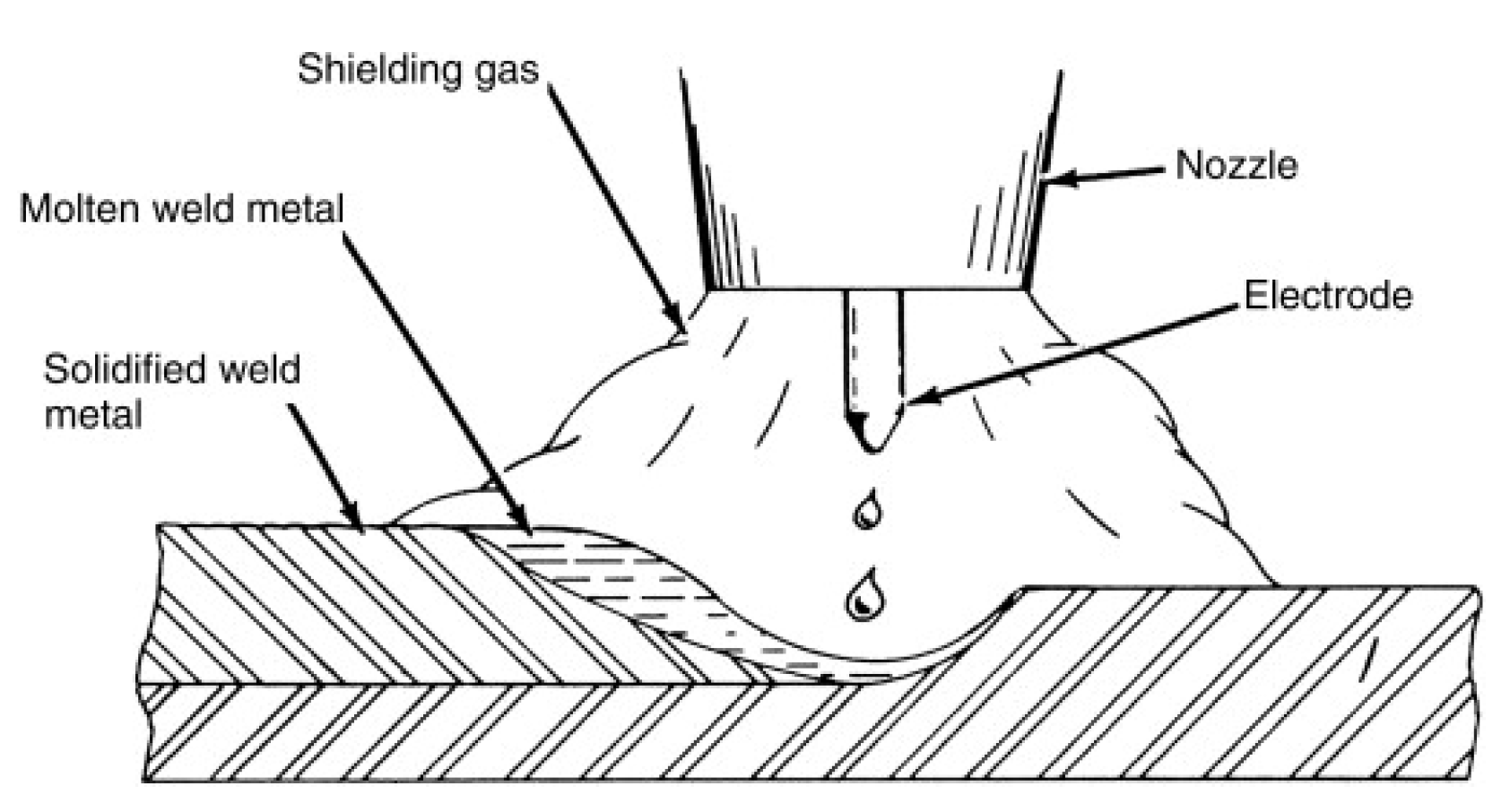
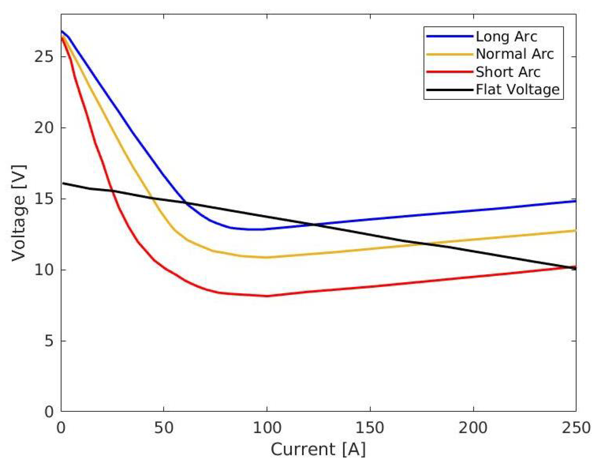
Review of GMAW Process and Defects

The welding process is based on a localized heat source that allows the melting of the materials. The intensity of the heat source determines the thermal transient and the mode of melting and re-solidification of the joint, on which the quality depends. The formula for specific heat input is as follows:

$$Q=\frac{I\ast V}{v_t}\ast \eta [\frac{\mathrm{J}}{\mathrm{mm}}]$$

(1)

The basic parameters to be monitored in a GMAW process are the welding speed $v_t$, the generator voltage V, and the arc-current I. In particular, the arc current is strongly variable with contact to workpiece distance (CTDW), wire feed rate, and wire properties, such as diameter and material [4] since the generator characteristic for this process is generally flat voltage, shown in Figure 2 [5].

Defects in welding are principal of two types:

• Metallurgical discontinuities, which are problematic primarily due to the drop in mechanical properties of the joint and are typically identified through nondestructive testing.
• Metallurgical inhomogeneity, which is more complex to identify and assess.

Typical defects include cracks, inclusions, and lack of penetration [6,7]. These defects are associated with unsuitable process parameters and, therefore, unsuitable specific heat. For example, if the specific heat is too low due to low current or high torch speed. In this case, there may be a lack of fusion of the edges to be welded or a lack of penetration, while high values of specific heat, associated with a low torch speed, may lead to the presence of cracks or metallurgical in-homogeneity. An inadequate value of specific heat supplied to the weld bead can also lead to the birth of inclusions, such as gaseous inclusions, which consist of gas entrapment in the weld pool due to too fast cooling associated with too high welding speeds. In the literature, a strong correlation between process parameters and defects is presented. Wei et al. showed the correlation between arc current and porosity [8]. Pal shows that current and voltage, which are correlated with acoustic emissions [9], are correlated with the depth of penetration and geometry aspect of the joint for a P-GMAW [10]. Additionally, the temperature and geometry of the arc are correlated with defects, as shown by Sreedhar [11] and Brobeg [12]. It is not always easy to check for defects in the joints, and this is a long and time-consuming job, especially when components are standardized and produced in large quantities. A sample check is carried out only on a few random samples in some sectors. In this case, artificial intelligence can be a viable method to evaluate the correct quality level for all components, including the items that skip the inspection stage. This is possible because the process parameters are directly involved in the defects rising, and these are all easily measurable. Shin et al. used different network architectures to correlate current and arc voltage to porosity, with an accuracy between 66–89% [13]. During gas metal arc welding, assuming that the generator has a flat voltage characteristic, slight variations in arc length lead to non-negligible fluctuations in the current affecting the arc: as the arc length increases, the current decreases, and vice versa, as seen in Figure 2.

In this case, the operator’s task—a human or a robotic arm—is to change parameters, such as the torch’s height from the workpiece, to bring these values back into range. This self-regulating characteristic of the electric arc leads to variations in current and, therefore, in the specific heat input supplied to the joint, which may cause defects in the items.

The Welding Procedure Specification (WPS) is a document that describes welding procedures and contains all the information needed to make quality welds. In the WPS, depending on the workpiece material, type of weld, and thickness, the welding parameters are provided, leading to a specific value for the heat input provided to it. For this work, information regarding process parameters such as current, voltage, and welding speed were collected from welds of different thickness in multi-pass welding, shown in Figure 3.

These values were compared with those in the WPS, which defines the best process parameters to reach a good quality of welded joint and that is obtained following experiments. The obtained errors were used to train a neural network. To the author’s best knowledge, this approach, inspired by control theory, is innovative in this field and helps training and so the performance because the error is a better variable to understand the meaning of the “high or low” process parameter, which is correlated to defects in the way presented before. The labels, necessary to train the supervised network, were obtained through non-destructive tests (NDTs), specifically ultrasonic and penetrant liquids tests, and we found the type and location of defects in the workpiece. In particular, ultrasonic testing allows us to find the depth at which a defect can be traced, which is the key to creating the labels for the multi-pass GMAW process. The schematic procedure used for this work is shown in Figure 4.

2. Materials and Methods

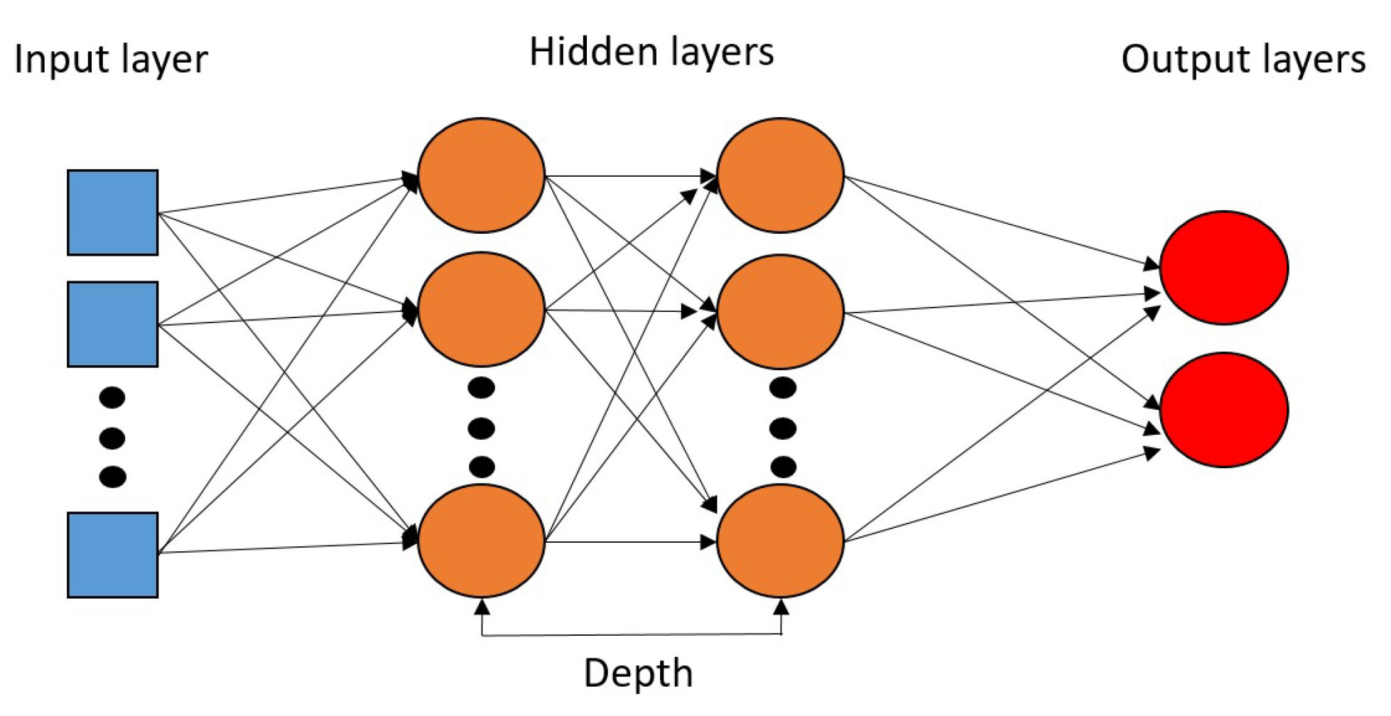
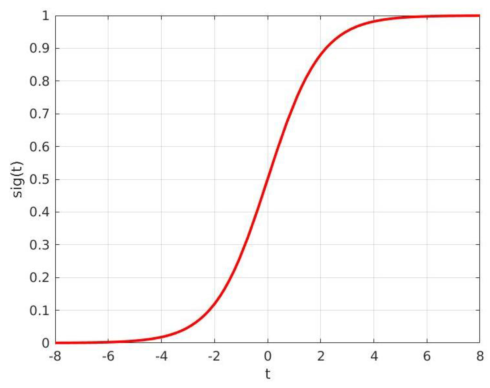
2.1. A Brief Summary of Artificial Neural Networks

Artificial neural networks (ANNs) are widely used in industry due to their ability to solve complex problems, such as image classification [14], audio classification [15], reinforcement learning [16], and to find patterns among a large amount of data [17]. Moreover, ANNs possess the ability to approximate any continuous function [18], and thus it is also used to derive models from data [19]. The basic structure of an ANN is a single layer perceptron (SLP) which consists of an input and an output layer, and it is the simplest ANN model, as shown in Figure 5.

However, this model cannot describe complex problems, so nowadays multilayer perceptron models (MLP) are mainly used, including more hidden layers between the input and output layers allow to overcome the limitations SLPs. The structure of an ANN MLP is shown in Figure 6.

The structure of an MLP, often called fully connected neural networks, is composed of many computational units defined as neurons, all connected through connections called weights. In particular, all the neurons of layer i are connected to those of layer $i-1$. Before passing to the next layer, the neuron’s output is eventually added with a constant (bias), which allows translating the value of a certain quantity. This output is passed through a non-linear activation function, a fundamental part that allows the neural network to approximate any continuous non-linear function.

Finding a useful network architecture for a specific task is not a trivial problem. It is a programmer’s job to choose the best architecture, network depth, number of neurons for each hidden-layers and activation function. Usually, this is done following a trial-and-error approach. It is also equally important to choose the optimization algorithm and the cost function to minimize that allows the neural network to learn the weights and biases and all hyperparameters like learning rate and regularization constants. For this purpose, gradient-based techniques of optimization find great use [20].

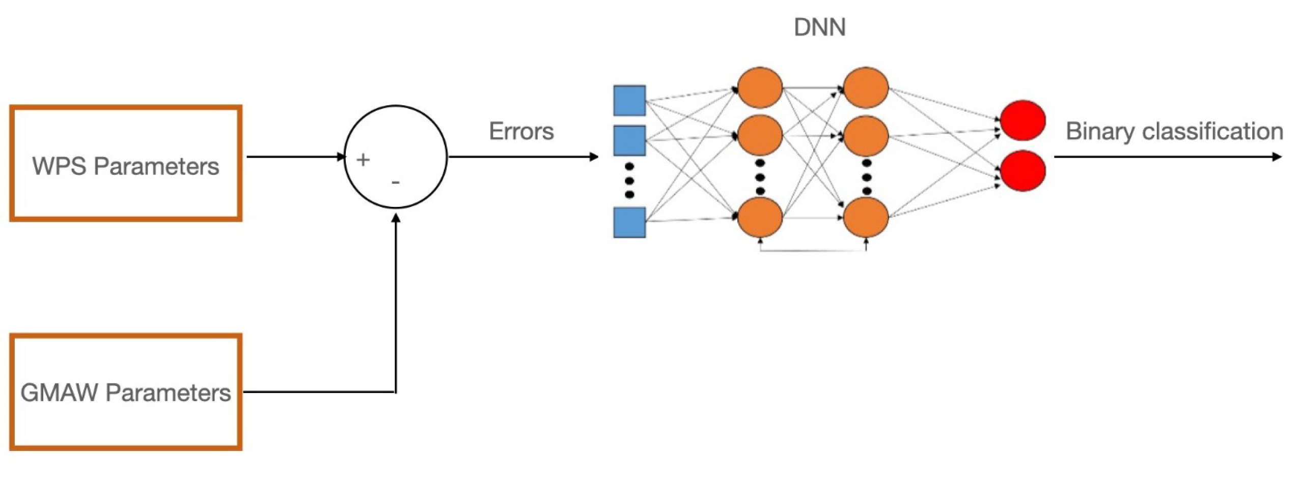
2.2. Development Workflow

In this work deviations of processing values from the optimal values described in the WPS were used as inputs to the neural network. Specifically, four inputs were used:

$$e_1=\mathrm{\Delta }{v}_{tmean}=v_{tmean}^{WPS}-v_t^{eff}$$

(2)

$$e_2=\mathrm{\Delta }{I}_{max}=I_{max}^{WPS}-I_{eff}$$

(3)

$$e_3=\mathrm{\Delta }{I}_{min}=I_{min}^{WPS}-I_{eff}$$

(4)

$$e_4=\mathrm{\Delta }{V}_{mean}=V_{mean}^{WPS}-V_{eff}$$

(5)

The output layer was characterized by a binary classification problem that associates 1 with adequate quality joints, as shown in Figure 4. In this work, we considered ten workpieces of 1 m of the length of a multi-pass gas metal arc welding with three different passes. We decided to slice each workpiece into 20 parts and acquire labels every 5 cm with NDT. With a sample time of $T_s=225$ ms, which is constrained from Miller acquisition hardware at a maximum of 0.1 s (Insight ArcAgent), we obtain 2655 samples that we used to train the neural network. The dataset is built by imposing a correspondence between the data acquired on each part section and the NDT result in the same section of 5 cm for all three passes of multi-pass welding. The hypothesis is that all data acquired in the same section have the same label. The references, namely the WPS, are known before the process and are equal for all pass and workpiece samples. NDTs are used to localize the defect (distance from the starting point and depth for identifying the pass) and correlate it with acquired sample parameters.

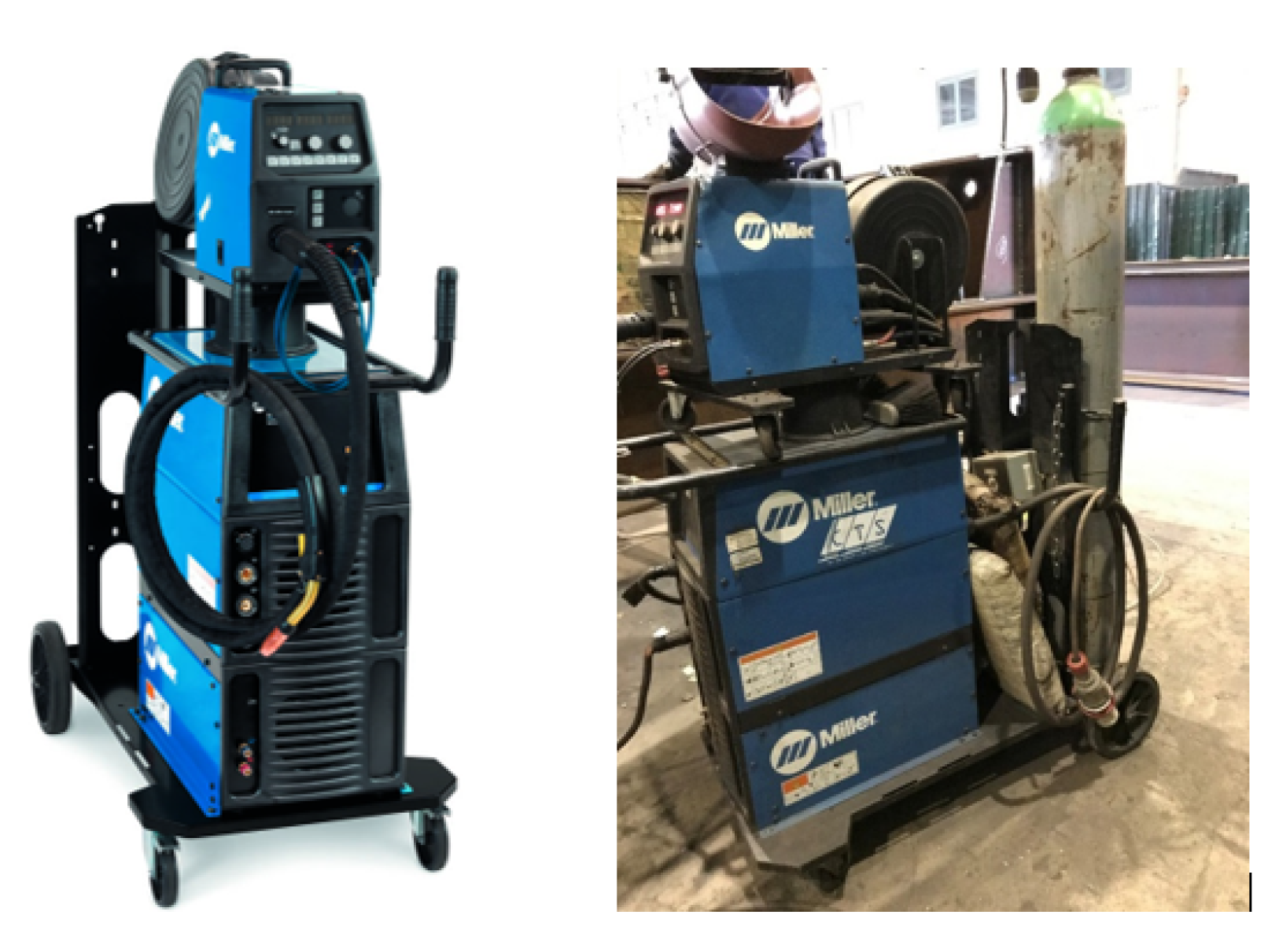
2.2.1. Case Study and Data Collection

The case study under consideration is based on the realization of welds on bases for an offshore plant on an FPSO vessel. No special materials were used for this work; almost all of the basement is made of S355J2 structural steel.

Multi-pass welds were performed using a Miller XMS 425 MPa in Figure 7 and a gas composed of 82% of argon and 18% carbon dioxide. The wire, with a 1.2 mm diameter, is AWS certified as A5.18:ER70S-6.

Miller Insight Core software was used to monitor welding operations and subsequent collection of welding parameters; this software allows monitoring in real-time and storing all the process parameters on a cloud. Together with the WPS, this data was exported in excel format and then pre-processed in a python environment.

Ultrasonic, magentoscopic, and penetrant liquids tests were performed on the welds. Figure 8 shows an image of one of the tests performed using penetrant liquids, which revealed the presence of a crater. Moreover, through an ultrasound inspection, it was possible to highlight a lack of fusion at a certain depth from the surface, corresponding to a certain welding pass to which certain welding parameters were associated. In this way, it was possible to assign labels to each welding pass whose process values were known. All of this information has been collected in a single file, which followed a pre-processing step in Python.

Pre-processing of the data involved scaling of the values to reference values for all process variables, to guarantee the same scale to all variables in input in neural network:

$$e_i=\frac{r-v_i}{r}$$

(6)

where r is the reference and $v_i$ the actual value of variable. So for each weld the scale errors were collected in a $4\times 1$ vector of features, and Equations (2)–(5) become:

$$e_1=\mathrm{\Delta }{v}_{tmean}=\frac{v_{tmean}^{WPS}-v_t^{eff}}{v_{tmean}^{WPS}}$$

(7)

$$e_2=\mathrm{\Delta }{I}_{max}=\frac{I_{max}^{WPS}-I_{eff}}{I_{max}^{WPS}}$$

(8)

$$e_3=\mathrm{\Delta }{I}_{min}=\frac{I_{min}^{WPS}-I_{eff}}{I_{min}^{WPS}}$$

(9)

$$e_4=\mathrm{\Delta }{V}_{mean}=\frac{V_{mean}^{WPS}-V_{eff}}{V_{mean}^{WPS}}$$

(10)

where $V^{WPS}$ is the voltage reported in the WPS and $V_{eff}$ is the measured voltage. The same is for the others parameters like welding speed $v_t$ and current I. Following the non-destructive tests, it was possible to associate the corresponding label with each feature vector corresponding to the single welding pass, as mentioned before.

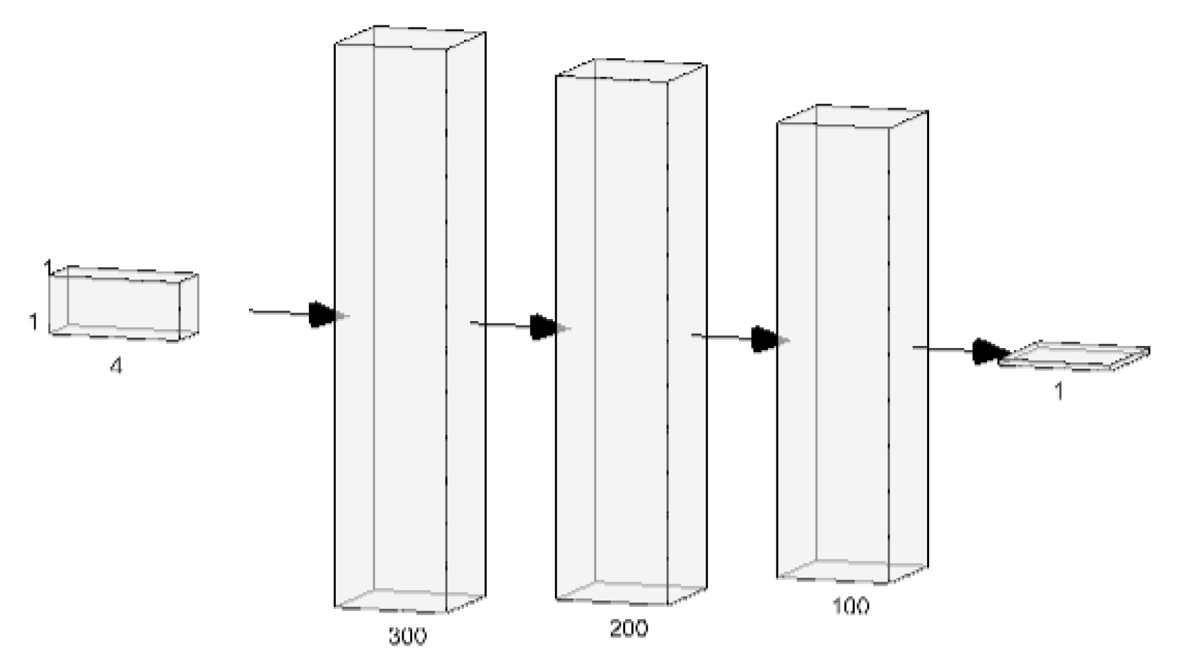
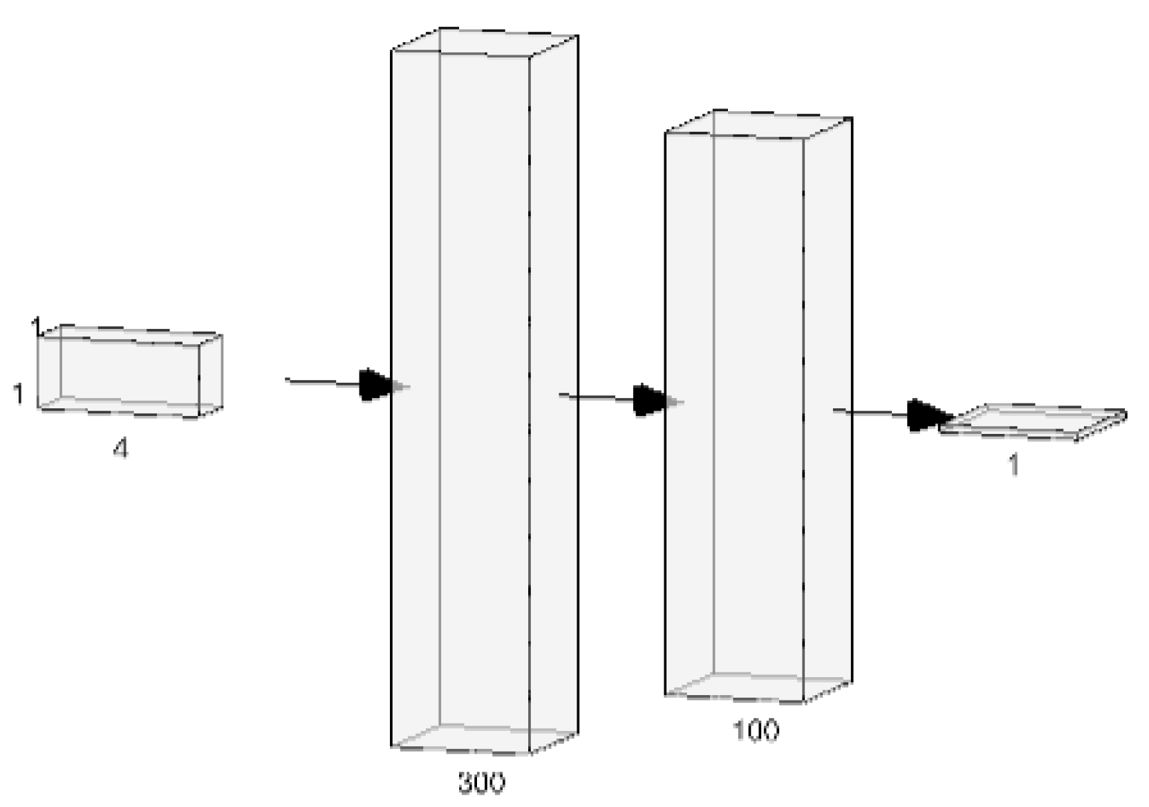
2.2.2. Choosing an Architecture

The chosen architecture is a multi-layer or fully connected network with a $4\times 1$ vector as the input layer and a binary value as output. For this reason, the activation function of the output layer will be a sigmoid, in Figure 9, since we solve a binary classification problem [21].

The sigmoid activation function is defined as follows, where t is the input parameter:

$$\sigma \left(t\right)=\frac{1}{1+e^{-t}}$$

(11)

This function allows us to transform an input between $[-\infty ,+\infty ]$ into a new one between [0, 1]. We associate with 1 the case of welding without defects. Probability 1-p is instead the one that describes the probability that the input feature vector is associated with a label 0.

Concerning the depth of the neural network, two different solutions have been studied. Architecture A consists of three hidden layers composed of [300, 200, 100] neurons in the different layers, where Architecture B consist in two hidden layer composed of [300, 100] neurons. These solutions are shown in Figure 10 and Figure 11.

The activation function chosen for each layer is a hyperbolic tangent, a function similar to sigmoid, shown in Figure 12.

$$\sigma \left(t\right)=\frac{e^t-e^{-t}}{e^t+e^{-t}}$$

(12)

This function allows us to transform an input between $[-\infty ,+\infty ]$ into a new one between [−1, 1], and is frequently used in ANN architectures [21].

For each layer, uniform Glorot distribution [22] was chosen as the initialization method for the weights because it is the most performing on activations functions sigmoid-like, such as the hyperbolic tangent function [23].

$$\mu =0;\sigma =\sqrt{\frac{2}{n_i+n_o}}$$

(13)

Finally between in the layer [n − 1] is add a dropout layer. The function of the dropout, whose results are shown in Figure 13, is to reduce the probability of overfitting by deleting random layer with a certainly probability [24].

2.2.3. Training

For the Architecture “A” there are 81,901 parameters to train, while for Architecure “B” 31,701. For the neural network training, a batch size of 64 was used to accelerate the training phase. The usage of the batches can be seen from the oscillation of the loss and accuracy graphs [25]. The optimization algorithm used is adaptive momentum estimation [26]. The learning rate is the most important hyper-parameter for training a neural network. Typically, the lrDecay technique is used to improve training performance and overcome problems due to the convexity of cost functions, reducing overfitting. You et al. [27] showed that an initially large learning rate suppresses the storage of noisy data while decaying the learning rate improves the learning of complex patterns. Therefore, a learning rate of $l{r}_{ini}=0.1$ and an exponential decay law were used:

$$lr=l{r}_{ini}\ast e^{-(step/decay)}$$

(14)

The main features of the training phase are summarized in

Table 1. Summary of hyper parameters of ANN.

Total samples	2655
Batch size	64
Initial learning rate ($l{r}_{ini}$)	$0.1$
Decay	6000
${\beta }_1$	$0.9$
${\beta }_2$	$0.99$
$ϵ$	1 × 10${}^{-7}$
Epochs	300
Step per epoch	35
Training size (% on the total)	$85\%$
Validation size (% on the total)	$10\%$

.

Figure 14 shows the exponential decay curve with $decay=6000$. With the chosen decay value, at the end of training, about 10,000 steps, the value taken by $lr=0.02$.

An NVIDIA GeForce GTX 1650—GDDR5 was used as the target for the training and subsequent inference phase, whose characteristics are shown in

Table 2. NVIDIA GeForce GTX 1650 characteristics.

Core NVIDIA CUDA	896
Boost Clock (MHz)	1665
Base Clock (MHz)	1485
Memory speed (Gbps)	8
Compute capability	$7.5$
Microarchitecture	Turing

:

Training and testing of the neural network were performed using the Tensorflow library [28].

3. Results

In the following, the loss function and accuracy trends during the training phase for the training and validation dataset are shown. Finally, for each solution, we report the confusion matrix associated with the test dataset, $5\%$ of the total, and the inference times for each solution.

3.1. Architecture A

Figure 15 and Figure 16 show the trends of the loss function and the accuracy of varying the epochs.

The results obtained at the end of the training and testing phase are shown in

Table 3. Principal results of Architecture A.

Final validation loss	$0.16$
Final training loss	$0.18$
Test accuracy	$93.6\%$
Inference time (ms)	$123.42$

:

Figure 17 shows the confusion matrix showing that $4.4\%$ of the defective joints were classified as compliant while $2\%$ of the compliant joints were classified as defective.

3.2. Architecture B

Figure 18 and Figure 19 show the trends of the loss function and the accuracy of varying the epochs for Architecture B.

The results obtained at the end of the training and testing phase are shown in

Table 4. Principal results of Architecture B.

Final validation loss	$0.13$
Final training loss	$0.15$
Test accuracy	$94.7\%$
Inference time (ms)	$93.9$

:

Figure 20 shows the confusion matrix showing that $1.5\%$ of the defective joints were classified as compliant while $3.8\%$ of the compliant joints were classified as defective.

Architecture B is the best solution due to the reduced inference time and the fewer non-conforming joints labeled as conforming, ensuring better performance and quality prediction confidence.

4. Conclusions and Future Developments

In this work, the welding parameters corresponding to each pass during multi-pass GMAW welding of offshore platform bases performed by a robotic axis were monitored. Subsequently, through non-destructive testing, it was possible to label the welds that did not show any defect, using different NDTs to find defects of different topologies. Once the dataset was generated, it was followed by a pre-processing activity, which led to obtaining four characteristic deviations of the welding parameters, acquired from the process with a sample rate of 225 ms, from those defined by the Welding Procedure Specification. With these deviations, a neural network with one or two hidden layers was trained, and the results were compared. At the end of the training phase, the neural network B presented 97% accuracy for joint classification. The proposed method is a novelty because is not only based on the usual data-driven approach of deep neural networks but is inspired by control theory with the concept of error. This new approach guarantees better results compared to other works, like that of Shin et al. [13], who proposed a similar approach with an accuracy of less than 90% for porosity detection. Furthermore, this network is also trained on different kinds of defects. These results represent a starting point for developing a more robust online quality control system for GMAW, which will be developed by integrating a camera in the inspection loop, which will allow the detection of other defects, including geometric ones during the welding process. However, in this work, only one type of material and wire were considered and is based on one type of WPS. To guarantee a generalization to any GMAW process more experiments must be conducted because the same error should not have the same influence on different materials, so other inputs could be considered, such as wire and workpiece material, joint temperature, gas flow rate, etc. The next step of this work could be the integration of other information like images and new experiments that lead to improving the performance and generalization capability of the network. After this, it will be possible to use the results in real-time for various purposes, such as the development of a new control logic for the feeder unit and robotic axis to adjust the parameters with the aim to avoid weld defects, which can work in the same loop with an intelligent monitoring system.

References

1. Xia, C.; Pan, Z.; Polden, J.; Li, H.; Xu, Y.; Chen, S. Modelling and prediction of Surface roughness in wire arc additive manufacturing using machine learning. J. Intell. Manuf. 2021, 1–16. [Google Scholar] [CrossRef]
2. Deng, H.; Cheng, Y.; Feng, Y.; Xiang, J. Industrial Laser Welding Defect Detection and Image Defect Recognition Based on Deep Learning Model Developed. Symmetry 2021, 13, 1731. [Google Scholar] [CrossRef]
3. Xia, C.; Pan, Z.; Zhang, S.; Li, H.; Xu, Y.; Chen, S. Model-free adaptive iterative learning control of melt pool width in wire arc additive manufacturing. Int. Adv. Manuf. Technol. 2020, 110, 2131–2142. [Google Scholar] [CrossRef]
4. Pan, J. Chapter 1: Dynamic behaviour of arc welding. In Arc Welding Control; Woodhead Publishing Ltd.: Cambridge, UK; CRC Press: Boca Raton, FL, USA, 2003; pp. 1–16. [Google Scholar]
5. Weman, L. Chapter 2: Equipment for MIG welding. In MIG Welding Guide; Woodhead Publishing Ltd.: Cambridge, UK; CRC Press: Boca Raton, FL, USA, 2006; pp. 29–35. [Google Scholar]
6. Weman, L. Chapter 9: Assessing weld quality in MIG welding. In MIG Welding Guide; Woodhead Publishing Ltd.: Cambridge, UK; CRC Press: Boca Raton, FL, USA, 2006; pp. 130–144. [Google Scholar]
7. Mathers, G. Weld defects and quality control. In The Welding of Aluminium and Its Alloys; Woodhead Publishing Ltd.: Cambridge, UK; CRC Press: Boca Raton, FL, USA, 2002; pp. 199–215. [Google Scholar]
8. Wei, E.; Farson, D.; Richardson, R.; Ludewig, H. Detection of Weld Surface Porosity by Statistical Analysis of Arc Current in Gas Metal Arc Welding. J. Manuf. Process. 2001, 3, 50–59. [Google Scholar] [CrossRef]
9. By, J.; Johnson, A.; Carlson, N.M.; Smartt, H.B.; Clark, D.E. Process Control of GMAW: Sensing of Metal Transfer Mode. Weld. J. 1991, 70, 91. [Google Scholar]
10. Pal, K.; Bhattacharya, S.; Pal, S.K. Investigation on arc sound and metal transfer modes for on-line monitoring in pulsed gas metal arc welding. J. Mater. Process. Technol. 2002, 210, 1397–1410. [Google Scholar] [CrossRef]
11. Sreedhar, U.; Krishnamurthy, C.V.; Balasubramaniam, K.; Raghupathy, V.D.; Ravisankar, S. Automatic defect identification using thermal image analysis for online weld quality monitoring. J. Mater. Process. Technol. 2012, 212, 1557–1566. [Google Scholar] [CrossRef]
12. Brobeg, P. Surface crack detection in welds using thermography. NDT & E Int. 2013, 57, 69–73. [Google Scholar] [CrossRef]
13. Shin, S.; Jin, C.; Yu, J.; Rhee, S. Real-Time Detection of Weld Defects for Automated Welding Process Base on Deep Neural Network. Metals 2020, 10, 389. [Google Scholar] [CrossRef] [Green Version]
14. Du, R.; Xu, Y.; Hou, Z.; Shu, J.; Chen, S. Strong noise image processing for vision-based seam tracking in robotic gas metal arc welding. Int. J. Adv. Manuf. Technol. 2019, 101, 2135–2149. [Google Scholar] [CrossRef]
15. Nanni, L.; Maguolo, G.; Brahnam, S.; Paci, M. An Ensemble of Convolutional Neural Networks for Audio Classification. Appl. Sci. 2021, 11, 5796. [Google Scholar] [CrossRef]
16. Jin, Z.; Li, H.; Gao, H. An intelligent weld control strategy based on reinforcement learning approach. Int. J. Adv. Manuf. Technol. 2019, 100, 2163–2175. [Google Scholar] [CrossRef]
17. Chiroma, H.; Abdullahi, U.A.; Alarood, A.A.; Gabralla, L.A.; Rana, N.; Shuib, L.; Hashem, I.A.; Gbenga, D.E.; Abubakar, A.I.; Zeki, A.M.; et al. Progress on Artificial Neural Networks for Big Data Analytics: A Survey. IEEE Access 2019, 7, 70535–70551. [Google Scholar] [CrossRef]
18. Hornik, K. Approximation capabilities of multilayer feedforward networks. Neural Netw. 1991, 4, 251–257. [Google Scholar] [CrossRef]
19. Selmic, R.R.; Lewis, F.L. Neural-network approximation of piecewise continuous functions: Application to friction compensation. IEEE Trans. Neural Netw. 2002, 13, 745–751. [Google Scholar] [CrossRef] [Green Version]
20. Ojha, V.K.; Abraham, A.; Snášel, V. Metaheuristic design of feedforward neural networks: A review of two decades of research. Eng. Appl. Artif. Intell. 2017, 60, 97–116. [Google Scholar] [CrossRef] [Green Version]
21. Rasamoelina, A.D.; Adjailia, F.; Sinčák, P. A Review of Activation Function for Artificial Neural Network. In Proceedings of the IEEE 18th World Symposium on Applied Machine Intelligence and Informatics (SAMI), Herlany, Slovakia, 23–25 January 2020; pp. 281–286. [Google Scholar] [CrossRef]
22. Bengio, Y.; Glorot, X. Understanding the difficulty of training deep feed forward neural networks. In Proceedings of the International Conference on Artificial Intelligence and Statistics, Sardinia, Italy, 13–15 May 2010; pp. 249–256. [Google Scholar]
23. Datta, L. A Survey on Activation Functions and their relation with Xavier and He Normal Initialization. arXiv 2020, arXiv:abs/2004.06632. [Google Scholar]
24. Srivastava, N.; Hinton, G.; Krizhevsky, A.; Sutskever, I.; Ruslan, S. Dropout: A Simple Way to Prevent Neural Networks from Overfitting. J. Mach. Learn. Res. 2014, 15, 1929–1958. Available online: http://jmlr.org/papers/v15/srivastava14a.html (accessed on 21 February 2022).
25. Gao, F.; Zhong, H. Study on the Large Batch Size Training of Neural Networks Based on the Second Order Gradient. arXiv 2020, arXiv:2012.08795. [Google Scholar]
26. Kingma, D.P.; Ba, J. Adam: A Method for Stochastic Optimization. arXiv 2014, arXiv:1412.6980. [Google Scholar]
27. You, K.; Long, M.; Wang, J.; Jordan, M. How does learning rare decay help modern neural networks? arXiv 2019, arXiv:1908.01878. [Google Scholar]
28. Tensorflow. Available online: https://www.tensorflow.org/ (accessed on 10 November 2021).
Figure 1. GMAW process.
Applsci 12 03615 g001
Figure 2. Self-autoregularization of arc current with constant voltage characteristics.
Applsci 12 03615 g002
Figure 3. Multi-pass welding.
Applsci 12 03615 g003
Figure 4. Procedure of training used in this work.
Applsci 12 03615 g004
Figure 5. Single layer perceptron architecture.
Applsci 12 03615 g005
Figure 6. Multilayer perceptron architecture.
Applsci 12 03615 g006
Figure 7. Miller XMS 425 MPa welding machine.
Applsci 12 03615 g007
Figure 8. Penetrant liquid inspection result.
Applsci 12 03615 g008
Figure 9. Sigmoid function.
Applsci 12 03615 g009
Figure 10. Architecture A.
Applsci 12 03615 g010
Figure 11. Architecture B.
Applsci 12 03615 g011
Figure 12. Hyperbolic tangent activation function.
Applsci 12 03615 g012
Figure 13. Dropout layer: (a) a standard neural network (b) the same network after dropout.
Applsci 12 03615 g013
Figure 14. Exponential decay of learning rate.
Applsci 12 03615 g014
Figure 15. Accuracy trend for Architecture A.
Applsci 12 03615 g015
Figure 16. Loss trend for Architecture A.
Applsci 12 03615 g016
Figure 17. Confusion matrix of Architecture A.
Applsci 12 03615 g017
Figure 18. Accuracy trend for Architecture B.
Applsci 12 03615 g018
Figure 19. Loss trend for Architecture B.
Applsci 12 03615 g019
Figure 20. Confusion matrix of Architecture B.
Applsci 12 03615 g020