Article

Object Detection for Industrial Applications: Training Strategies for AI-Based Depalletizer

by
Domenico Buongiorno
1,2,
Donato Caramia
1,
Luca Di Ruscio
3,
Nicola Longo
2,3,
Simone Panicucci
3,
Giovanni Di Stefano
3,
Vitoantonio Bevilacqua
1,2,* and
Antonio Brunetti
1,2
1
Department of Electrical and Information Engineering (DEI), Polytechnic University of Bari, 70126 Bari, Italy
2
Apulian Bioengineering s.r.l., Via delle Violette 14, 70026 Modugno, Italy
3
Comau S.p.A., Via Rivalta 30, 10095 Grugliasco, Italy
*
Author to whom correspondence should be addressed.
Appl. Sci. 2022, 12(22), 11581; https://doi.org/10.3390/app122211581
Submission received: 17 October 2022 / Revised: 3 November 2022 / Accepted: 10 November 2022 / Published: 15 November 2022
(This article belongs to the Special Issue Machine Learning in Manufacturing Technology and Systems)

Abstract

:
In the last 10 years, the demand for robot-based depalletization systems has constantly increased due to the growth of sectors such as logistics, storage, and supply chains. Since the scenarios are becoming more and more unstructured, characterized by unknown pallet layouts and stock-keeping unit shapes, the classical depalletization systems based on the knowledge of predefined positions within the pallet frame are going to be substituted by innovative and robust solutions based on 2D/3D vision and Deep Learning (DL) methods. In particular, the Convolutional Neural Networks (CNNs) are deep networks that have proven to be effective in processing 2D/3D images, for example in the automatic object detection task, and robust to the possible variability among the data. However, deep neural networks need a big amount of data to be trained. In this context, whenever deep networks are involved in object detection for supporting depalletization systems, the dataset collection represents one of the main bottlenecks during the commissioning phase. The present work aims at comparing different training strategies to customize an object detection model aiming at minimizing the number of images required for model fitting, while ensuring reliable and robust performances. Different approaches based on a CNN for object detection are proposed, evaluated, and compared in terms of the F1-score. The study was conducted considering different starting conditions in terms of the neural network’s weights, the datasets, and the training set sizes. The proposed approaches were evaluated on the detection of different kinds of paper boxes placed on an industrial pallet. The outcome of the work validates that the best strategy is based on fine-tuning of a CNN-based model already trained on the detection of paper boxes, with a median F1-score greater than 85.0 % .

1. Introduction

The current state of robotics and Artificial Intelligence (AI) allows for the replacement of repetitive labor with automation, resulting in significant growth opportunities for efficiency and cost. As the worldwide economy recovers post-pandemic, the demand for labor has outstripped supply, in particular in strongly growing fields such as logistics and fulfillment [1]. In these sectors, the need to create an efficient and flexible supply chain, capable of satisfying the needs of the individual citizen, has been highlighted.
Automation in the handling and storage of goods plays a fundamental role in optimizing the supply chain; those activities include repetitive and time-consuming tasks that do not add value to the finished product. Consequently, automating these tasks [2,3] through the usage of advanced robotic solutions [4,5,6] can streamline the entire supply chain and provide a better-quality service to the citizens. In addition, this would allow operators to dedicate themselves to more complex tasks that are less subject to physiologically unfavorable postures. Among the set of available technologies, the interest around automated systems for depalletization is constantly increasing. This is due to the fact that depalletization is a very monotonous, strenuous, and sometimes, quite dangerous task [7,8].
Automated systems for depalletization are in charge of picking stock-keeping units from a pallet and placing them in an handling system, such as a conveyor. The first depalletization systems were based on fixed positions in space; thus, they required being programmed for each specific pallet layout. Since industrial scenarios are becoming more and more unstructured, currently, these systems are becoming obsolete as they do not provide a sufficient level of flexibility. Consequently, innovative depalletization systems based on computer vision and artificial intelligence are growing in popularity, since they are able to complete the task while requiring the least amount of information.
In the last few years, many vision-based depalletizing techniques have been developed and proposed by the research community. The traditional approaches considered the processing of both 2.5D or 3D data of the scene by means of standard techniques mainly based on the extraction of geometric keypoints and 3D vertices or edges with the aim to solve an object matching problem for 3D pose estimation [9,10,11,12,13,14,15,16,17,18,19].
In recent years, new approaches based on deep convolutional neural networks have been proposed and investigated. In 2018, Schwarz et al. [20] presented a solution that combined three depth streams into one common frame. Schwarz et al. used a convolutional neural network, based on the DenseCap network, to perform the object detection of a 2D image. They used deep learning techniques to train their model, but the large number of parameters and the training set size to learn the feature were limitations. Using transfer learning, they solved this problems. In 2020, Caccavale et al. [21] developed a flexible robotic depalletizing system for supermarkets, which used the Intel Realsense RGB-D camera to acquire the scene with the pallet. Supported by transfer learning, they trained a CNN model to recognize food boxes in the RGB image. They used the depth information to perform the pose estimation. Fontana et al. [22] (2021) used a vision system composed by a Sick Visionary-S depth camera, which was mounted at a 1.80 m height from the conveyor belt and observed the parcel boxes directly from above. Such a depth camera combines structure light patterns and stereo vision in order to acquire RGB image and 3D point clouds. The Mask R-CNN was used to detect the parcel boxes within the 2D image, which are objects without texture and always have an orthogonal planar face. The bounding boxes of the detected boxes were used to select a region of interest in the point clouds, and such a selected RoI was used to estimate the pose of the objects. The information regarding the algorithm for the pose estimation was not treated. Opaspilai et al. [23] (2021) used a 2D camera to classify and locate pharmaceutical products. Using the 2D camera, the depalletizer was not able to detect the size of objects; for this reason, the authors improved the depalletizer using the 3D camera. The 3D camera was the Intel Realsense depth camera D435 with a 1920 × 1080 resolution for RGB and a 1280 × 720 resolution for the depth sensor. Both solutions used YOLOv3 as the CNN model to detect the object. The 3D pose estimation was not treated. Zhang et al. [24] (2022) used RGB-D data to classify and locate several objects. The architecture of their pose estimator was composed by a segmentation module, used to obtain the mask of the object in order to crop the 2D image and the point clouds. Then, the point clouds were managed by PointNet, which extracted the geometry features, while the 2D image was sent to a CNN to perform the edge extraction. The outputs of the PointNet and CNN were used in the Dense Fusion block to produce the 3D pose estimation.
All the recent review papers about automatic vision-based depalletization systems propose a two-step approach, which consists of detecting the object within a 2D image and then elaborating the portion of the point cloud extracted by using the 2D RoI to estimate the pose of the specific object that has to be manipulated by a robot. Such a choice is mainly motivated by the high performance of the deep CNN, along with the advantages of transfer learning, in detecting different kinds of objects within a 2D image. Leveraging this aspect, most of the authors used a CNN pretrained on popular datasets, e.g., ImageNet and COCO, to fine-tune custom object detectors, mainly focusing on the final performance. However, to the best of authors’ knowledge, the authors in this field did not focus on two main aspects that are important when a company has to develop a customized system for a new client, which are (a) the number of images of the custom setup that have to be acquired to train the CNN model and (b) the specific transfer learning approach that will lead to better performance. Compared with the traditional feature-based approaches, it has been proven in many application fields that the deep neural networks require a big amount of training data [25,26,27,28,29,30]. Collecting big datasets in industrial environments is usually a time-consuming activity, which implies a substantial increase of the commissioning time. Regarding the transfer learning procedure, a possible approach might consider fine-tuning a network pretrained on datasets such as ImageNet or COCO with the new images collected by the system; however, an alternative method could contemplate adding another step of fine-tuning in the middle by using images of similar stock-keeping units, which, for example, could have been acquired with the same sensor.
Envisaging an automatic vision-based depalletization system featuring the two processing steps described above and able to manipulate paper boxes, in this work, the authors studied and compared a set of possible approaches that could be followed to reach the desired performances on a custom AI-based object detection model for depalletization considering a variable training set size. The model takes as the input 2D images of a pallet loaded with paper boxes, and it is in charge of detecting all the boxes that have to be reached and grasped by the picking robot. By using different in-house datasets of paper boxes lying on a pallet, three different training approaches were considered: (1) the first regards the fine-tuning of a model pretrained on the COCO Dataset by using the images of the new paper boxes to be detected; (2) the second considers the training of a model pretrained on the COCO Dataset by using only images of paper boxes that are different from the new paper boxes; (3) the third one regards the fine-tuning of the model already fine-tuned at the previous point with images of the new paper boxes. It is worth reporting that, in this work, the authors focused only on the object detection step and, then, did not investigate and describe the step that concerns the 3D pose estimation.
The article is organized as follows: Section 2 describes the dataset, detector, data augmentation, and experimental design used during the study; the outcomes of the experimental studies are provided and discussed in Section 3; finally, the concluding remarks are presented in Section 4.

2. Materials and Methods

The section provides information about the collected in-house datasets and presents the CNN architecture employed to train the models with ML techniques, the experimental design, and the statistics approaches for the performance comparisons.

2.1. Datasets

All the images that compose the datasets used in this study were collected with a custom setup reported in Figure 1. The employed camera sensor was the PhoXi 3D Scanner XL [31], which captures 2D images and 3D point clouds. The camera was mounted 3.3 m away from the floor. The PhoXi 3D Scanner XL is suitable for depalletizer applications since it ensures a large scanning volume. Three different datasets were acquired:
1.
Dataset 1, Figure 2A, composed of 1160 labeled images and 3712 paper boxes, containing only Comau® boxes characterized by several shapes and poses. All the paper boxes are white and present the same logo.
2.
Dataset 2, Figure 2B, composed of 1907 labeled images and 11,566 paper boxes, containing boxes characterized by several prints, logos, shapes, and poses. The boxes belonging to this dataset are different from each other.
3.
Dataset 3, Figure 2C, composed of 889 labeled images and 7575 paper boxes, containing white boxes without prints and logos, characterized by two possible shapes, and placed such that all the most-extended faces are parallel to the floor.
All the boxes of each dataset were manually labeled with the class box by using the Computer Vision Annotation Tool (CVAT) [32], which allows multiple types and formats of annotations. The labeling procedure was performed considering the following guidelines:
1.
The label should be adhered as tightly as possible to the box, and the box must be inscribed within the label.
2.
If any part of the box is occluded by another box, such that you can only see less than 90% (approximately) of the occluded box, exclude that box from being labeled.
3.
Avoid labeling any boxes with less than 3 corners visible.
4.
If a single box shows more than a single face, the most-extended face must be labeled.
5.
The RoI of the boxes must have the sides parallel with the sides of the image.

2.2. The Employed Object Detection Model as Part of the Depalletization System

The depalletizer solution considered in this work leverages 2D images and 3D point clouds. In this specific case, both types of data were acquired by exploiting the same sensor, i.e., the PhoXi 3D Scanner XL [31]. The depalletization process starts with a 2D and 3D scan of the environment. The image acquired is processed by an object detection model, which is in charge of detecting all the visible stock-keeping units, i.e., paper boxes, in the image. For each paper box that has been found, a bounding box that fully inscribes it is computed. Exploiting the mapping between the 2D image and 3D point cloud, the bounding boxes will then be employed to extract the portion of the point cloud containing the box. The extracted 3D portion of point cloud is supposed to be further processed in order to estimate the pose of the specific paper box to grasp and manipulate. It is worth noting that the object detection step is really important in order to extract the majority of the 3D points that belong to the specific paper box, minimizing, at the same time, the number of 3D points of other boxes. Thus, the quality of the 2D RoI resulting from the object detection step has a big impact on the 3D pose estimation accuracy and on the complexity of the estimation procedures.

2.2.1. The EfficientDet-D0 Architecture

The authors considered the EfficientDet-D0 architecture because of both its relatively high performance on COCO, with respect to the Average Precision (AP) metric ( A P , A P 50 , A P 75 equal to 34.6 , 53.0 , 37.1 , respectively) and, especially, its very low inference time, i.e., 10.2 ms with an NVIDIA® Tesla® V100 [33]. In fact, both the number of parameters and the FLOP value of the selected architecture are very low and equal to 3.9 M and 2.5 B, respectively. It is worth reporting that such values of the AP are related to the 91 classes of the COCO Dataset and are lower for almost 20% with respect to the performance of the best EfficientDet-D7 [33], which is characterized by an inference time equal to 122 ms (exploiting the same GPU card), a FLOP value equal to 325 B and 52 M of the parameters. Considering the fact that the studied application is based on only one object class and that time is a critical resource in the depalletization system, in the authors’ opinion, the D0 version represents a good solution. Moreover, by running several inference tests on a workstation based on an i7 family CPU (32 GB RAM, Intel® Core i7-9700E processor and an Integrated Intel® UHD graphics 630), it emerged that the average inference time was equal to 0.652 s. The inference time represents 7.70% of the whole process, starting from the 2D and 3D scans of the environment to the pick and place and assuming a robot movement time of 5 s.
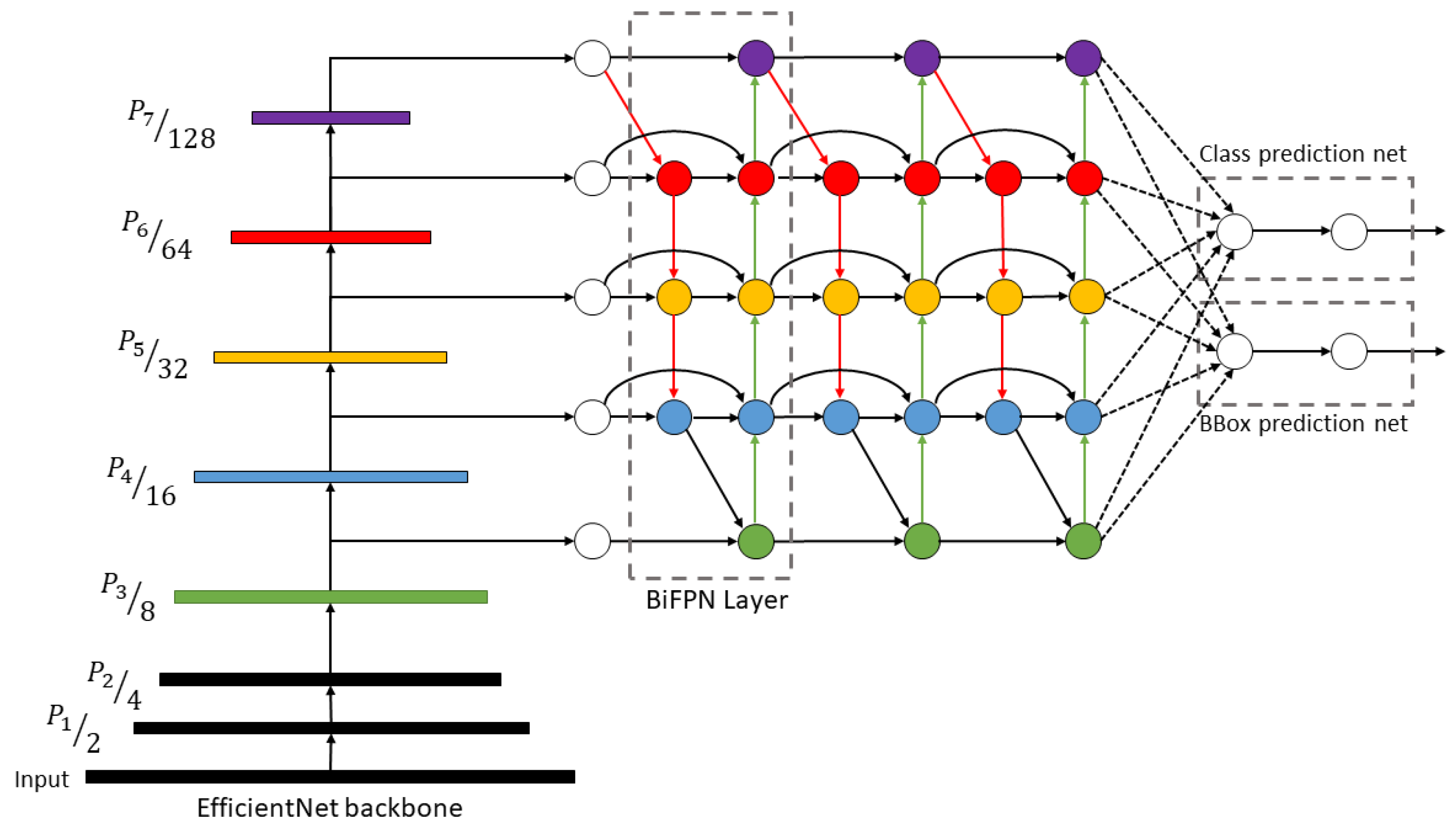
Figure 3 shows EfficientDet’s architecture [33], which is the one-stage detector. EfficientNet-B0 was employed as the backbone network, with the transfer learning of ImageNet. This architecture presents a novel feature network, the BiFPN, which takes Level 3–7 features { P 3 , P 4 , P 5 , P 6 , P 7 } from the backbone network and applies bottom-up and top-down bidirectional feature fusion several times. These fused features are the input of the class and box prediction layers, which perform the object classification and bounding box.
The backbone network adopts the same width/depth scaling coefficient of EfficientNet-B0 [34] such that it is easy to reuse the pretrained ImageNet checkpoints. The BiFPN has a width and depth:
W B i F P N = 64 ( 1 . 35 ϕ ) = 64 , D B i F P N = 3 + ϕ = 3
keeping in mind that ϕ = 0 for EfficientDet-D0. The box/class prediction network has a width and depth, respectively:
W p r e d = W B i F P N = 64 , D b o x = D c l a s s = 3 + i n t ( ϕ / 3 ) = 3
The input image resolution must be divisible by 2 7 since Feature Levels 3–7 were used, and for this reason, R i n p u t is calculated using the equation below:
R i n p u t = 512 + 128 · ϕ = 512

2.2.2. Training the CNN Model

In this case study, the employed CNN model was trained several times (as will be discussed below—Section 2.4), and for each training, the adopted stopping criterion was the total number of epochs, which was set to 100 epochs. Furthermore, Stochastic Gradient Descent with Momentum (SGDM) was used as optimization algorithm to update the model’s state with a momentum value equal to 0.9. All the other considered hyperparameters were set according to [33].
In this work, the authors used the Model ZOO of TensorFlow Object Detection (TFOD) API [35], which is an open-source framework built on top of TensorFlow, which makes it easy to create, train, and deploy accurate machine learning models capable of localizing and identifying multiple objects in a single image. The Model ZOO of TFOD provides several checkpoints, which were generated from training on the COCO [36] Dataset and are useful to initialize the weights of the CNN. The TFOD API allows training the model by using three different modalities:
1.
Classification: Initialize the classification backbone weights, in our case the EfficientNet backbone, with the same weights of the pretrained model on the COCO Dataset, while the BiFPN layers and class/box prediction layers are randomly initialized.
2.
Detection: Initialize the classification backbone and BiFPN weights with the same weights of the pretrained model on the COCO Dataset. The box/class prediction layers are randomly initialized.
3.
Full: Initialize the entire detection model, including the EfficientNet backbone, BiFPN, and box and class prediction layers with the same weights as the pretrained model on the COCO Dataset.
For each of the above modalities, it is possible train the entire detection model, just the BiFPN and box/class weights, or just the box/class weights.

2.3. Data Augmentation

As will be discussed in the Experimental Design Subsection (Section 2.4), some of the performed trainings considered the usage of data augmentation, which is a well-known technique, which can be used to artificially expand the size of a training dataset by creating modified versions of the original images. In this work, the data augmentation steps that were applied in series were:
a
Random brightness and contrast with the probability to be applied equal to 0.5;
b
Horizontal and vertical flip with the probability to be applied equal to 0.5.

2.4. Experimental Design

In this section, we clearly explain the experimental design in order to present the proposed approaches, the training set size, and the dataset used for each training.

2.4.1. Proposed Approaches

The goal of this work was to evaluate and compare different approaches, also called “cases” throughout the text, that could be used to train a model able to detect new boxes within a 2D image. Such a situation can occur when commissioning a depalletizing system at a new facility. In particular, the authors considered the following approaches (see Figure 4):
1.
Considering the model already pretrained on the COCO Dataset, using the detection modality (see Section 2.2.2) and updating the whole detection model:
  • [Case 1a]—To fine-tune the model with images of the new boxes;
  • [Case 1b]—To fine-tune the model with images of the new boxes and using the above-mentioned data augmentation strategy;
2.
[Case 2a]—Considering the model already pretrained on the datasets of images containing different boxes with the detection modality and no frozen layers (see Section 2.2.2), to test the model on new images without any further fine-tuning or training;
3.
Considering the model already pretrained on the datasets of images containing different boxes, using the full modality and the feature extractor frozen (see Section 2.2.2):
  • [Case 3a]—To fine-tune the model with images of the new boxes;
  • [Case 3b]—To fine-tune the model with images of the new boxes and synthetic copies generated with data augmentation.
The different proposed approaches that were reported above were all evaluated considering a different number of training images and exactly the same test set characterized by a fixed size. In detail, each training without DA was performed by increasing the number of training images as follows: k = { 15 , 29 , 58 , 116 , 232 , 464 , 696 , 928 } , whereas each training with DA was run with the following training set sizes: k = { 45 , 87 , 174 , 348 , 696 , 1392 , 2088 , 2784 } . The size of the test set was always equal to 232.

2.4.2. Experiment Conditions

The comparison among the proposed approaches was performed considering two different conditions, which differed in terms of the datasets employed for training and testing. The two conditions evaluated were:
  • [Dataset 1]—Dataset 1 (see the Datasets Subsection) was considered as the new dataset (the test set included only images of Dataset 1), whereas Dataset 2 and Dataset 3 were used to pretrain the model when evaluating Case 3;
  • [Dataset 2]—Dataset 2 (see the Datasets Subsection) was considered as the new dataset (the test set included only images of Dataset 2), whereas Dataset 1 and Dataset 3 were used to pretrain the model when evaluating Case 3.
The two experimental conditions Dataset 1 and Dataset 2 were designed according to the following principles:
  • Case 3 of both experimental conditions must have in common the training on Dataset 3 since it contains the images of neutral white paper boxes without any logo or texture;
  • An experimental condition must focus on the detection of boxes characterized by a simple texture; this is the case of Dataset 1, which considers the detection of the paper boxes of Dataset 1 based on white boxes with the same logo;
  • The other experimental condition must focus on boxes featuring more complex textures with a high inter-variability among the boxes in terms of texture and shape; this is the case of Dataset 2, which considers the detection of the paper boxes of Dataset 2 based on boxes characterized by different kinds of prints, logos, and shapes.

2.5. Cross-Validation

Cross-validation was adopted for both conditions Dataset 1 and Dataset 2, using 1160 data samples from each considered dataset. Both datasets were split into 5 folds F = { f 1 , f 2 , f 3 , f 4 , f 5 } , each one containing n = 232 labeled images. In order to be balanced, every fold presented about the same number of box labels. For each training session, four folds were used to compose the training set, and the remaining one was used as a test set.

2.6. Performance Metric

In this work, the authors considered both the Average Precision ([email protected], with I o U = 0.5 ) and Recall (AR) as equally important. Thus, the chosen metric was the F1-score [37] since it is the harmonic mean between them, calculated using equation:
F 1 - score = 2 · 1 1 AP @ 0.5 + 1 AR
The selected performance metrics were computed for each testing fold to obtain the distribution of the confidence interval.

2.7. Comparisons and Statistics

This section illustrates the working guidelines used for the results’ evaluation. Starting from the experimental results, two different comparisons were considered: Comparison I illustrates, for each scenario, what happens when increasing the training set size; Comparison II compares the F1-score among all the scenarios given a specific number of new images.
For the statistic analysis, the non-parametric Friedman test was chosen. The non-parametric Friedman test and Dunn’s pairwise post hoc test with Bonferroni correction were carried out using the medians to compare the scores for the different comparisons, to check the statistically significant results. In fact, the Friedman test identifies the differences in terms of the ranks between each pair of groups tested; once having adjusted the p-values with Bonferroni correction, if the p-values are less than the statistical significance level (0.05), it allows for pairwise comparisons.

3. Results and Discussion

3.1. Comparison I Results

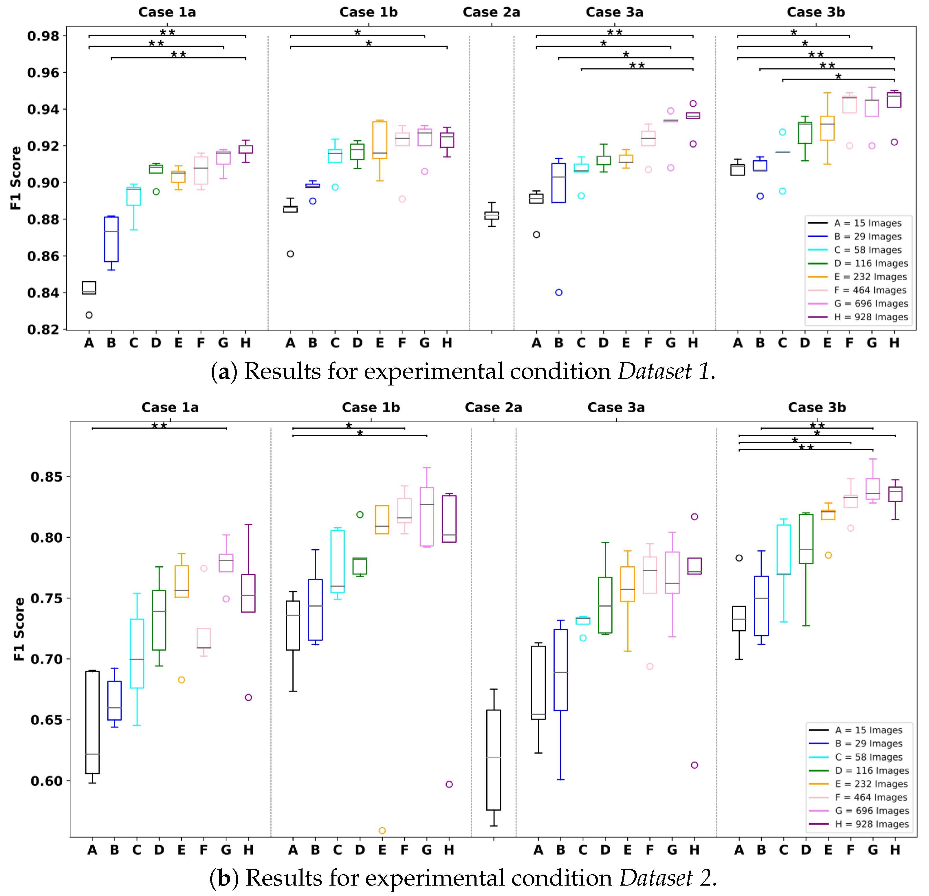
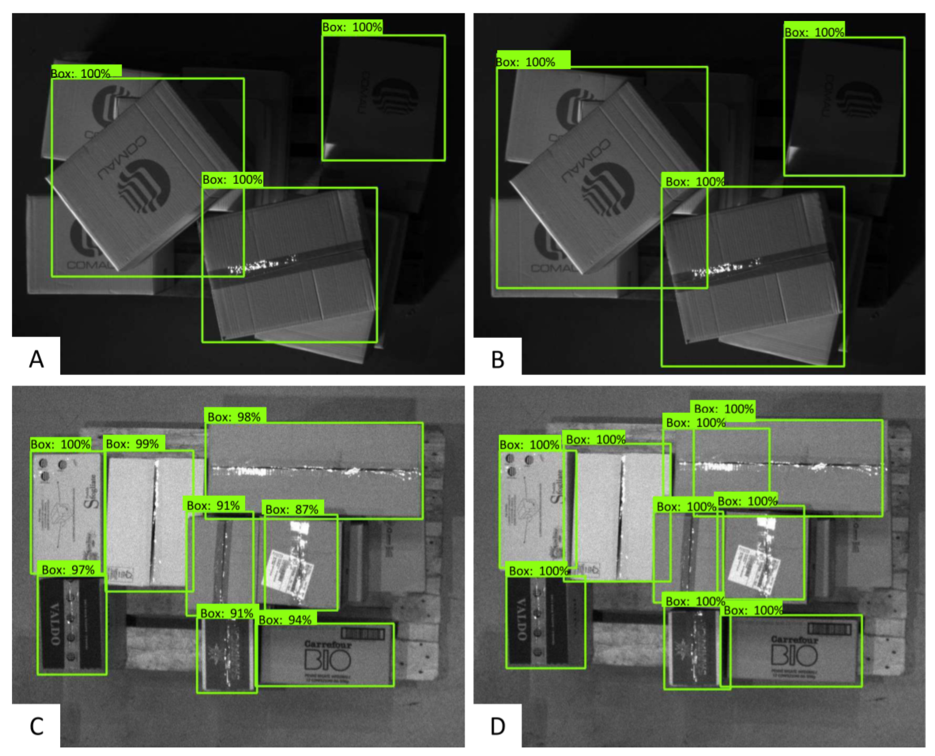
Considering Comparison I, Figure 5a shows the experimental results obtained on Dataset 1. For each approach, the F1-score improved when increasing the number of images. In particular, in Case 1a, the median F1-score varied from 84.0 % to 92.0 % , and in Case 3b, the median F1-score increased from 90.9 % to 94.7 % . Figure 6A,B highlight the differences in terms of the detection obtained from the models. It can be noticed that the model characterized by the highest F1-score provided a bounding box that was closer to the corners of the boxes.
Figure 5b (Dataset 2) highlights the same trend: in Case 1a, the median F1-score increased from 60.6 % to 75.2 % and in Case 3b from 73.3 % to 83.8 % . Figure 6C,D highlight the differences in terms of the detection of the models. In can be noticed that the model characterized by the highest F1-score was more accurate during the detection. Moreover, it provided bounding boxes closer to the edges of the boxes.
Analyzing Dataset 1, in Case 1a, there were statistically significant differences between A and H, A and G, and B and H with p-values of 0.0002 , 0.0034 , and 0.0043 , respectively. Case 1b presented a statistical difference between A and G with p = 0.0149 and between A and H with p = 0.0182 . For Case 3a, the F1-score was different between A and H, A and G, B and H, and C and H, in particular with p = 0.0008 , p = 0.0116 , p = 0.0165 , and p = 0.0022 . Regarding Case 3b, there were statistical differences between A and F ( p = 0.0432 ), A and G ( p = 0.0261 ), A and H ( p = 0.0016 ), B and H ( p = 0.0077 ), and C and H ( p = 0.0327 ). Regarding Dataset 2, in Case 1a, the F1-score distributions of A and G were statistically different ( p = 0.0053 ). For Case 1b, the statistical differences were between A and F and A and G with p = 0.0258 and p = 0.0395 , respectively. Case 3b had four statistical differences, B and G ( p = 0.0099 ), A and H ( p = 0.0202 ), A and F ( p = 0.0352 ), and A and G ( p = 0.0037 ). It is worth noting that, in most of the cases, there was a significant difference between the F1-score obtained with the biggest training sets, e.g., G and H, and the F1-score obtained with the smallest training sets, e.g., A and B. Even if a growing trend can be observed for each case/approach, there were no significant differences when comparing the results achieved with the medium-sized training sets and the ones obtained with both the biggest and smallest sizes. In the authors’ opinion, such results are mainly motivated by the Bonferroni correction due to the high number of multiple comparisons.
When comparing the results of the two conditions, Dataset 1 and Dataset 2, it is worth noting that the F1-score values obtained for Dataset 2 were lower. In the authors’ opinion, Dataset 2 contains boxes that are more difficult to correctly detect due to the richness of the textures and prints. This can be stated observing the results of both Cases 1a and 1b (the models were pretrained with the COCO Dataset) and Cases 3a and 3b (the models were pretrained with images of different boxes). The same difference is reported when comparing Case 2a.

3.2. Comparison II Results

In this subsection, the comparisons among the cases, or approaches, are reported and discussed. Table 1 reports all the pairwise comparisons that were statistically different when comparing the F1-score among all the cases given a fixed size of the training set. Such an analysis was conducted on both experimental conditions, Dataset 1 and Dataset 2.
First of all, considering the trends reported in Figure 5a and Table 1, it can obliviously be stated that the data augmentation was always preferable if, of course, the computation resources can manage a bigger training set within a reasonable time. This can be noticed by comparing Case 1a vs. Case 1b and Case 3a vs. Case 3b, given a fixed training size. Most of such differences were not statistically significant due to the Bonferroni correction for multiple comparison, but can easily be observed within Figure 5a. This finding is true for both experimental conditions Dataset 1 and Dataset 2.
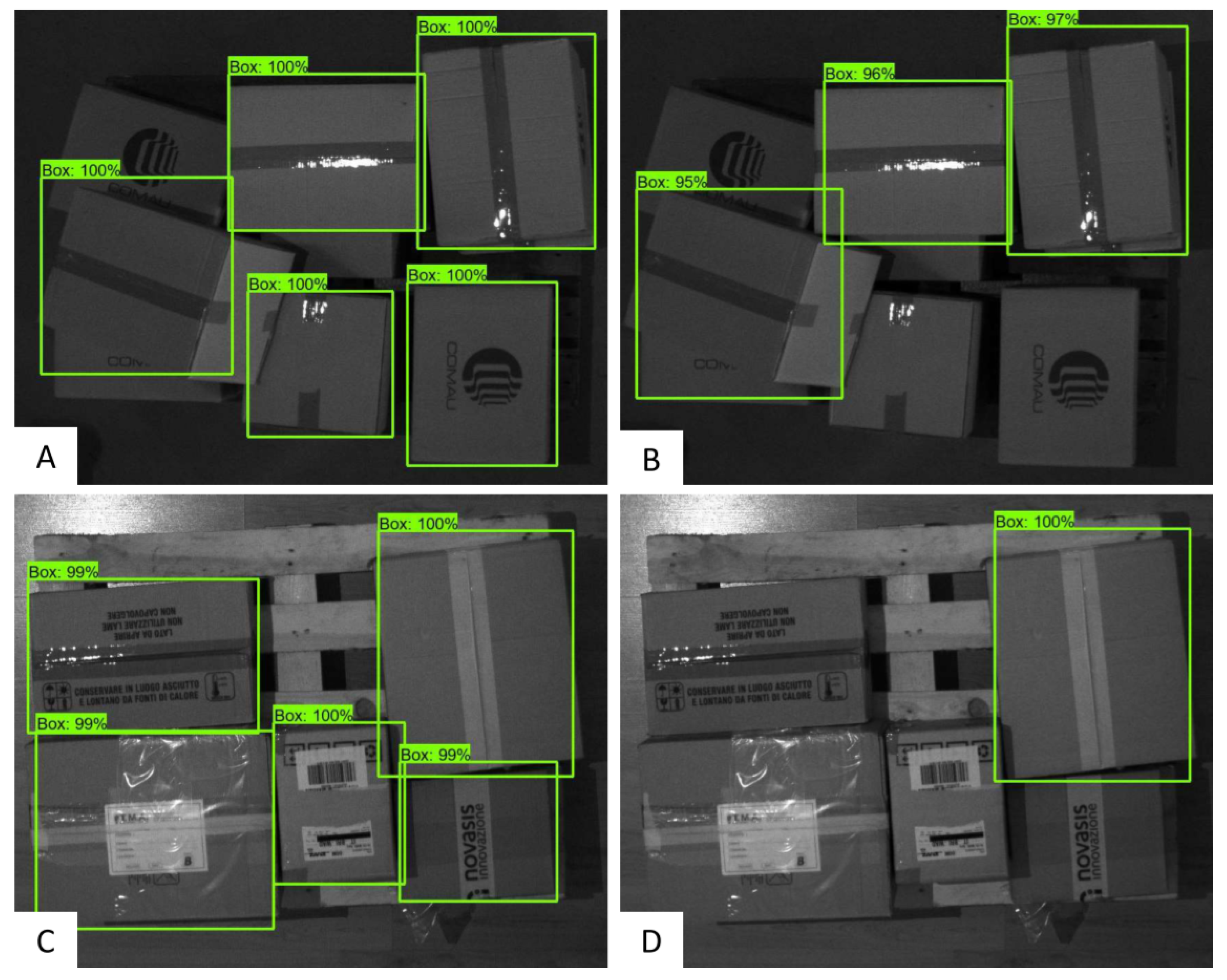
Another important aspect concerns the results of Case 2a, which studied the possibility of using a pretrained network on other dataset of different boxes without performing fine-tuning on the new box images. Comparing Case 2a with the two Case 3s (Case 3a and Case 3b), it emerged that the fine-tuning always allowed reaching better performances, and this was true for both experimental conditions Dataset 1 and Dataset 2 and for most of the training sizes, as shown in Figure 7. Figure 7A,B highlight the differences between Approaches 2a and 3b considering Dataset 1: the model of Case 2a was not able to deal with new boxes, while the model of Case 3b, fine-tuned on a new boxes, correctly detected all the visible boxes. Figure 7C shows the improved predictions related to the fine-tuning of a pretrained model with Dataset 2; Figure 7D highlights the missed prediction of the model with Dataset 2, due to the difficulty for the model to predict boxes with multiple textures and prints. However, comparing Case 2a with the two Case 1s (Case 1a and Case 1b), something different occurred. For the condition Dataset 1, i.e., the new dataset contained simple boxes to be detected, it emerged that the results of Case 2a (the pretrained network was trained also with more complex boxes) were comparable to or better than the results of the Case 1s for a training set size smaller that 30 images, whereas, for the condition Dataset 2, i.e., the new dataset contained complex boxes to be detected, it turned out that the results of Case 2a (the pretrained network was trained only with simple boxes) were always worse than the results of the Case 1s. This result is another important hint that can be considered when approaching the design and commissioning of a new depalletizer system.

4. Conclusions

The presented paper proposed an analysis regarding several training strategies for an object detection model that can be employed in order to reduce the commissioning time associated with an AI-based depalletizer system. The authors proposed the usage of a CNN for object detection supported by the Tensorflow Object Detection API. Several scenarios were taken into account to evaluate, using the F1-score as the unique metric, which was the one that ensured reliable detection performances, minimizing the training set size. Additionally, a comparison among several optimization strategies was carried out, keeping fixed the number of original images that composed the training set. It was demonstrated that, by exploiting a transfer learning training strategy and data augmentation techniques, robust detection accuracy was achieved while minimizing the amount of data needed for training, thus reducing the commissioning time associated with the depalletizer solution.

Author Contributions

Conceptualization, D.B., A.B., N.L., G.D.S., S.P. and V.B.; methodology, D.C., D.B., L.D.R., N.L. and S.P.; software, D.C., D.B., L.D.R., N.L. and S.P.; validation, D.C., D.B., L.D.R., N.L. and S.P.; formal analysis, D.C., D.B., L.D.R., N.L. and S.P.; investigation, D.B., A.B., N.L. and S.P.; data curation, D.C., L.D.R., N.L. and S.P.; writing—original draft preparation, all authors; writing—review and editing, all authors; visualization, D.B., D.C., L.D.R., N.L. and S.P.; supervision, D.B., N.L. and S.P.; funding acquisition, G.D.S. and V.B. All authors have read and agreed to the published version of the manuscript.

Funding

This research was partially funded by the Public-Private Laboratory “Cognitive Diagnostics” between the Polytechnic University of Bari and Comau® S.p.A. company.

Institutional Review Board Statement

Not applicable.

Informed Consent Statement

Not applicable.

Data Availability Statement

Data are not available due to data protection.

Conflicts of Interest

The authors declare no conflict of interest.

References

  1. Ballou, R.H. The evolution and future of logistics and supply chain management. Eur. Bus. Rev. 2007, 19, 332–348. [Google Scholar] [CrossRef] [Green Version]
  2. Tommila, T.; Ventä, O.; Koskinen, K. Next generation industrial automation–needs and opportunities. Autom. Technol. Rev. 2001, 2001, 34–41. [Google Scholar]
  3. Bangemann, T.; Karnouskos, S.; Camp, R.; Carlsson, O.; Riedl, M.; McLeod, S.; Harrison, R.; Colombo, A.W.; Stluka, P. State of the art in industrial automation. In Industrial Cloud-Based Cyber-Physical Systems; Springer Nature Switzerland AG: Cham, Switzerland, 2014; pp. 23–47. [Google Scholar]
  4. Gavrilovskaya, N.V.; Kuvaldin, V.P.; Zlobina, I.S.; Lomakin, D.E.; Suchkova, E.E. Developing a robot with computer vision for automating business processes of the industrial complex. J. Phys. Conf. Ser. 2021, 1889, 022024. [Google Scholar] [CrossRef]
  5. Parmar, H.; Khan, T.; Tucci, F.; Umer, R.; Carlone, P. Advanced robotics and additive manufacturing of composites: Towards a new era in Industry 4.0. Mater. Manuf. Process. 2022, 37, 483–517. [Google Scholar] [CrossRef]
  6. Ribeiro, J.; Lima, R.; Eckhardt, T.; Paiva, S. Robotic Process Automation and Artificial Intelligence in Industry 4.0—A Literature review. Procedia Comput. Sci. 2021, 181, 51–58. [Google Scholar] [CrossRef]
  7. Lucas, R.A.I.; Epstein, Y.; Kjellstrom, T. Excessive occupational heat exposure: A significant ergonomic challenge and health risk for current and future workers. Extrem. Physiol. Med. 2014, 3, 1–8. [Google Scholar] [CrossRef] [PubMed] [Green Version]
  8. Kumar, B.; Gupta, V. Industrial automation: A cost effective approach in developing countries. Int. J. Res. Eng. Appl. Sci. 2014, 4, 73–79. Available online: https://www.researchgate.net/publication/301728845_Industrial_Automation_A_Cost_Effective_Approach_In_Developing_Countries (accessed on 1 July 2022).
  9. Baerveldt, A.J. Contribution to the Bin-Picking Problem. Robust Singulation of Parcels with a Robot System Using Multiple Sensors; ETH Zürich: Zürich, Switzerland, 1993. [Google Scholar]
  10. Katsoulas, D.; Kosmopoulos, D. An efficient depalletizing system based on 2D range imagery. In Proceedings of the 2001 ICRA. IEEE International Conference on Robotics and Automation (Cat. No.01CH37164), Seoul, Korea, 21–26 May 2001; Volume 1, pp. 305–312. [Google Scholar]
  11. Vayda, A.; Kak, A. A robot vision system for recognition of generic shaped objects. CVGIP Image Underst. 1991, 54, 1–46. [Google Scholar] [CrossRef]
  12. Katsoulas, D.; Bergen, L.; Tassakos, L. A versatile depalletizer of boxes based on range imagery. In Proceedings of the 2002 IEEE International Conference on Robotics and Automation (Cat. No.02CH37292), Washington, DC, USA, 11–15 May 2002; Volume 4, pp. 4313–4319. [Google Scholar]
  13. Rothwell, C.A.; Zisserman, A.; Forsyth, D.A.; Mundy, J.L. Planar object recognition using projective shape representation. Int. J. Comput. Vis. 1995, 16, 57–99. [Google Scholar] [CrossRef]
  14. Rahardja, K.; Kosaka, A. Vision-based bin-picking: Recognition and localization of multiple complex objects using simple visual cues. In Proceedings of the IEEE/RSJ International Conference on Intelligent Robots and Systems. IROS ’96, Osaka, Japan, 4–8 November 1996; Volume 3, pp. 1448–1457. [Google Scholar]
  15. Papazov, C.; Haddadin, S.; Parusel, S.; Krieger, K.; Burschka, D. Rigid 3D geometry matching for grasping of known objects in cluttered scenes. Int. J. Robot. Res. 2012, 31, 538–553. [Google Scholar] [CrossRef]
  16. Drost, B.; Ulrich, M.; Navab, N.; Ilic, S. Model globally, match locally: Efficient and robust 3D object recognition. In Proceedings of the 2010 IEEE Computer Society Conference on Computer Vision and Pattern Recognition, San Francisco, CA, USA, 13–18 June 2010; pp. 998–1005. [Google Scholar]
  17. Choi, C.; Taguchi, Y.; Tuzel, O.; Liu, M.Y.; Ramalingam, S. Voting-based pose estimation for robotic assembly using a 3D sensor. In Proceedings of the 2012 IEEE International Conference on Robotics and Automation, St. Paul, MN, USA, 14–18 May 2012; pp. 1724–1731. [Google Scholar]
  18. Holz, D.; Topalidou-Kyniazopoulou, A.; Stückler, J.; Behnke, S. Real-time object detection, localization and verification for fast robotic depalletizing. In Proceedings of the 2015 IEEE/RSJ International Conference on Intelligent Robots and Systems (IROS), Hamburg, Germany, 28 September–3 October 2015; pp. 1459–1466. [Google Scholar]
  19. Aleotti, J.; Baldassarri, A.; Bonfè, M.; Carricato, M.; Chiaravalli, D.; Di Leva, R.; Fantuzzi, C.; Farsoni, S.; Innero, G.; Lodi Rizzini, D.; et al. Toward Future Automatic Warehouses: An Autonomous Depalletizing System Based on Mobile Manipulation and 3D Perception. Appl. Sci. 2021, 11, 5959. [Google Scholar]
  20. Schwarz, M.; Milan, A.; Periyasamy, A.S.; Behnke, S. RGB-D object detection and semantic segmentation for autonomous manipulation in clutter. Int. J. Robot. Res. 2018, 37, 437–451. [Google Scholar] [CrossRef] [Green Version]
  21. Caccavale, R.; Arpenti, P.; Paduano, G.; Fontanellli, A.; Lippiello, V.; Villani, L.; Siciliano, B. A Flexible Robotic Depalletizing System for Supermarket Logistics. IEEE Robot. Autom. Lett. 2020, 5, 4471–4476. [Google Scholar] [CrossRef]
  22. Fontana, E.; Zarotti, W.; Rizzini, D.L. A Comparative Assessment of Parcel Box Detection Algorithms for Industrial Applications. In Proceedings of the 2021 European Conference on Mobile Robots (ECMR), Bonn, Germany, 31 August–3 September 2021; pp. 1–6. [Google Scholar]
  23. Opaspilai, P.; Vongbunyong, S.; Dheeravongkit, A. Robotic System for Depalletization of Pharmaceutical Products. In Proceedings of the 2021 7th International Conference on Engineering, Applied Sciences and Technology (ICEAST), Pattaya, Thailand, 1–3 April 2021; pp. 133–138. [Google Scholar]
  24. Zhang, Y.; Liu, Y.; Wu, Q.; Zhou, J.; Gong, X.; Wang, J. EANet: Edge-Attention 6D Pose Estimation Network for Texture-Less Objects. In Proceedings of the IEEE Transactions on Instrumentation and Measurement, Ottawa, ON, Canada, 16–19 May 2022; Volume 71, pp. 1–13. [Google Scholar]
  25. Bevilacqua, V.; Pietroleonardo, N.; Triggiani, V.; Brunetti, A.; Di Palma, A.M.; Rossini, M.; Gesualdo, L. An innovative neural network framework to classify blood vessels and tubules based on Haralick features evaluated in histological images of kidney biopsy. Neurocomputing 2017, 228, 143–153. [Google Scholar] [CrossRef]
  26. Cascarano, G.D.; Loconsole, C.; Brunetti, A.; Lattarulo, A.; Buongiorno, D.; Losavio, G.; Sciascio, E.D.; Bevilacqua, V. Biometric handwriting analysis to support Parkinson’s Disease assessment and grading. BMC Med. Inform. Decis. Mak. 2019, 19, 1–11. [Google Scholar] [CrossRef] [PubMed] [Green Version]
  27. Bevilacqua, V.; Buongiorno, D.; Carlucci, P.; Giglio, F.; Tattoli, G.; Guarini, A.; Sgherza, N.; De Tullio, G.; Minoia, C.; Scattone, A.; et al. A supervised CAD to support telemedicine in hematology. In Proceedings of the 2015 International Joint Conference on Neural Networks (IJCNN), Killarney, Ireland, 12–17 July 2015; pp. 1–7. [Google Scholar]
  28. Altini, N.; De Giosa, G.; Fragasso, N.; Coscia, C.; Sibilano, E.; Prencipe, B.; Hussain, S.M.; Brunetti, A.; Buongiorno, D.; Guerriero, A.; et al. Segmentation and Identification of Vertebrae in CT Scans Using CNN, k-Means Clustering and k-NN. Informatics 2021, 8, 40. [Google Scholar] [CrossRef]
  29. Buongiorno, D.; Trotta, G.F.; Bortone, I.; Di Gioia, N.; Avitto, F.; Losavio, G.; Bevilacqua, V. Assessment and Rating of Movement Impairment in Parkinson’s Disease Using a Low-Cost Vision-Based System. In Proceedings of the Intelligent Computing Methodologies, Wuhan, China, 15–18 August 2018; Huang, D.S., Gromiha, M.M., Han, K., Hussain, A., Eds.; Springer International Publishing: Cham, Switzerland, 2018; pp. 777–788. [Google Scholar]
  30. Bevilacqua, V.; Salatino, A.A.; Di Leo, C.; Tattoli, G.; Buongiorno, D.; Signorile, D.; Babiloni, C.; Del Percio, C.; Triggiani, A.I.; Gesualdo, L. Advanced classification of Alzheimer’s disease and healthy subjects based on EEG markers. In Proceedings of the 2015 International Joint Conference on Neural Networks (IJCNN), Killarney, Ireland, 12–16 July 2015; pp. 1–5. [Google Scholar]
  31. Photoneo. PhoXi 3D Scanner XL. Available online: https://www.photoneo.com/products/phoxi-scan-xl/ (accessed on 1 July 2022).
  32. Sekachev, B.; Manovich, N.; Zhiltsov, M.; Zhavoronkov, A.; Kalinin, D.; Hoff, B.; Osmanov, T.; Kruchinin, D.; Zankevich, A.; Sidnev, D.; et al. Opencv/Cvat: V1.1.0. 2020. Available online: https://zenodo.org/record/4009388#.Y3JJT3bMK38 (accessed on 1 June 2022).
  33. Tan, M.; Pang, R.; Le, Q.V. EfficientDet: Scalable and Efficient Object Detection. In Proceedings of the IEEE/CVF Conference on Computer Vision and Pattern Recognition (CVPR), Seattle, WA, USA, 14–19 June 2020. [Google Scholar]
  34. Tan, M.; Le, Q. EfficientNet: Rethinking Model Scaling for Convolutional Neural Networks. In Proceedings of the 36th International Conference on Machine Learning, Long Beach, CA, USA, 9–15 June 2019; Volume 97, pp. 6105–6114. [Google Scholar]
  35. Huang, J.; Rathod, V.; Sun, C.; Zhu, M.; Korattikara, A.; Fathi, A.; Fischer, I.; Wojna, Z.; Song, Y.; Guadarrama, S.; et al. Speed/accuracy trade-offs for modern convolutional object detectors. arXiv 2016, arXiv:1611.10012. Available online: http://xxx.lanl.gov/abs/1611.10012 (accessed on 1 July 2022).
  36. Lin, Y.T.; Maire, M.; Belongie, S.; Hays, J.; Perona, P.; Ramanan, D.; Dollár, P.; Zitnick, C.L. Microsoft COCO: Common Objects in Context. arXiv 2014, arXiv:1405.0312. [Google Scholar]
  37. Sepúlveda, J.; Velastin, S.A. F1-score assesment of Gaussian mixture background subtraction algorithms using the MuHAVi dataset. In Proceedings of the 6th International Conference on Imaging for Crime Prevention and Detection (ICDP-15), London, UK, 15–17 July 2015. [Google Scholar]
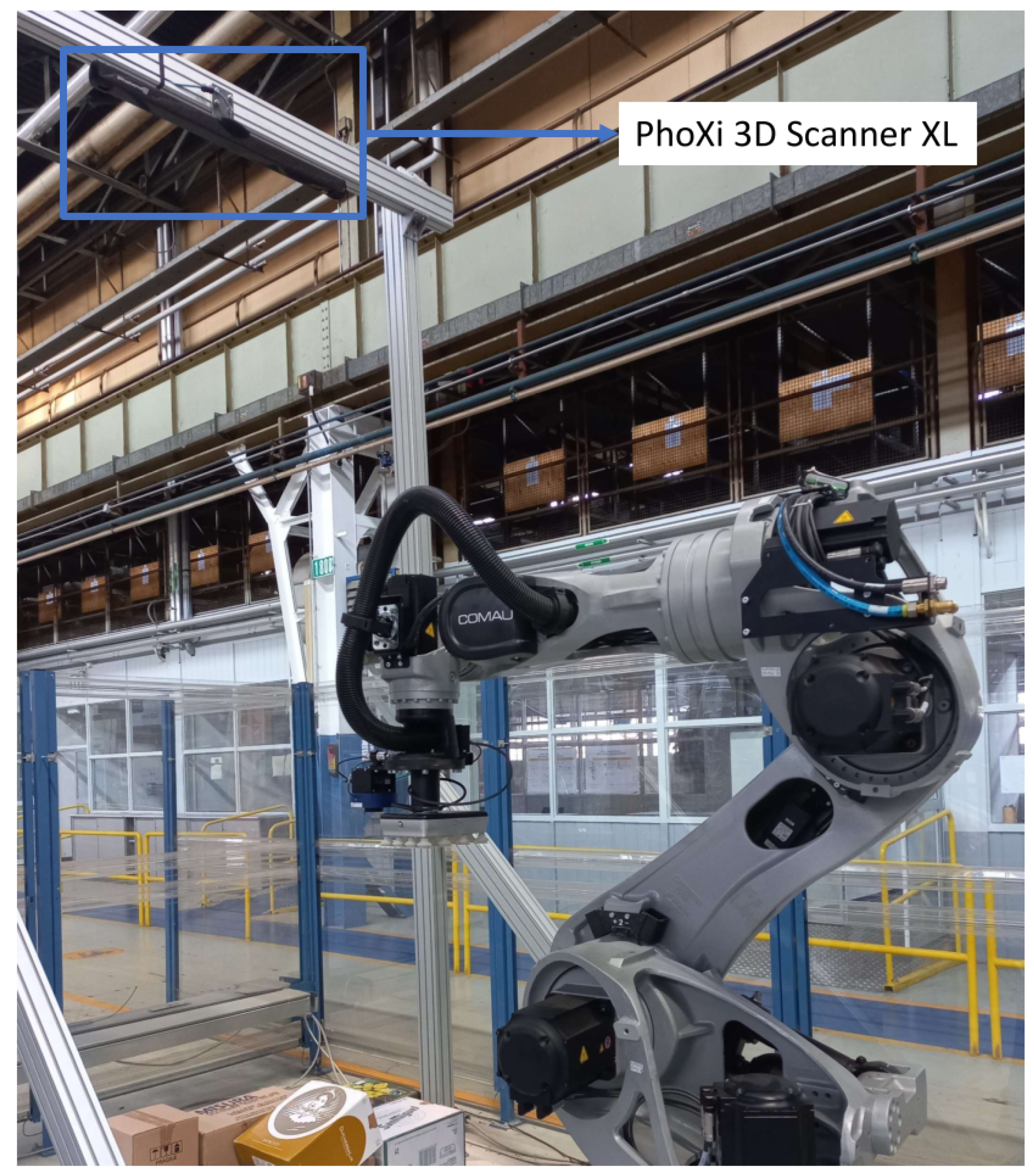
Figure 1. PhoXi 3D Scanner XL in the setup.
Applsci 12 11581 g001
Figure 2. Sample image of Dataset 1 (A). Sample image of Dataset 2 (B). Sample image of Dataset 3 (C).
Applsci 12 11581 g002
Figure 3. EfficientDet-D0 architecture. EfficientNet-B0 [34] is the backbone network; multiple BiFPN layers are the feature network and the class/box prediction network. The class and box prediction layers are repeated as many times as there are classes; in this work, the authors used just the class box.
Applsci 12 11581 g003
Figure 4. Scheme of the approaches.
Applsci 12 11581 g004
Figure 5. The boxplot of the F1-score distributions on the test sets for the comparison of a fixed scenario varying the training set size, considering Dataset 1 (a) and Dataset 2 (b). Case 1a, Case 1b, Case 2a, Case 3a, and Case 3b are the scenarios. A, B, C, D, E, F, G, and H are the numbers of the original images used for the training set. * represents statistically significant comparisons with p ≤ 0.05; ** represents p ≤ 0.01.
Applsci 12 11581 g005
Figure 6. (A) Sample result of the model fine-tuned on Dataset 1 with a median F1-score of 94.7 % . (B) Sample result of the model fine-tuned on Dataset 1 with a median F1-score of 90.9 % . (C) Sample result of the model fine-tuned on Dataset 2 with a median F1-score of 83.9 % . (D) Sample result of the model fine-tuned on Dataset 2 with a median F1-score of 73.3 % .
Applsci 12 11581 g006
Figure 7. (A) Sample result of the model fine-tuned on Dataset 1 considering Case 3b. (B) Sample result of the model fine-tuned on Dataset 1 considering Case 2a. (C) Sample result of the model fine-tuned on Dataset 2 considering Case 3b. (D) Sample result of the model fine-tuned on Dataset 2 considering Case 2a.
Applsci 12 11581 g007
Table 1. Statistically significant differences of Comparison II.
Training Set SizeDataset 1Dataset 2
Pairwise p Value Pairwise p Value
151a–3b0.00021b–2a0.0137
2a–3b0.0228
291a–3b0.00691b–2a0.0198
2a–3b0.0127
581b–2a0.01481b–2a0.0050
2a–3b0.01092a–3b0.0031
1161a–3b0.02742a–3b0.0036
2a–3b0.00161b–2a0.0080
2321a–3b0.02612a–3b0.0036
2a–3b0.0016
4642a–3b0.00061b–2a0.0036
2a–3b0.0008
6961a–3b0.02711b–2a0.0080
2a–3b0.00082a–3b0.0006
2a–3a0.0197
9282a–3a0.01092a–3b0.0016
2a–3b0.0009
Publisher’s Note: MDPI stays neutral with regard to jurisdictional claims in published maps and institutional affiliations.