Linear and Nonlinear Performance Analysis of Hydrodynamic Journal Bearings with Different Geometries

Abstract

In rotor dynamics, a traditional way of representing the dynamics of hydrodynamic bearings is using stiffness/damping coefficients. It is thus necessary to carry out a linearization of hydrodynamic forces around the shaft’s equilibrium position. However, hydrodynamic bearings have highly nonlinear nature, depending on operating conditions. Therefore, this paper discusses the applicability of these linear/nonlinear approaches using a computational model of the rotating system, where the finite element method is used for rotor modelling and the finite volume method for bearing calculation. The main goal is to investigate the boundaries for linear approximation of the hydrodynamic forces present in lobed hydrodynamic bearings, with the system operating under high loading conditions. Several numerical simulations were performed varying preload parameter and rotating speed. A comparison of the system’s responses, in time domain (shaft orbits) and frequency domain (full spectrum), is made for linear and nonlinear models. Results showed that trilobed bearings are more susceptible to nonlinearities, even in situations of smaller vibration amplitudes, while elliptical bearings are sensitive only under larger vibration amplitudes. These analyses are of great importance for mapping the influence of nonlinearities in different types of lobed hydrodynamic bearings with fixed geometry, varying the preload parameter to verify the influence on the system’s dynamic response. This study is important and serves as the basis for cases of monitoring and fault diagnosis (in the field of structural health monitoring) since it is crucial to distinguish what would be a fault signature or a standard nonlinear effect created by the use of hydrodynamic bearings.

1. Introduction

Hydrodynamic bearings play an important role in the dynamics of turbomachines and are widely used in industry because they allow high loads at low and high rotating speeds. The bearings properties highly influence the dynamic characteristics of a rotor, and instability phenomena tend to especially appear at high rotating speeds. The latest advances in the metal-mechanical industry have overcome most bearing machining problems. New materials and designs have brought increased bearing life, which are no longer the main reason for fault or malfunction in certain applications. Thus, the interactions of bearings with the surrounding mechanical system are drawing attention.

The dynamics of the bearing is mainly governed by support zones between its fixed and movable parts since these transmit all vibration between the fixed parts of the bearing and the moving parts of the system. Therefore, the oil film in these interfaces, mainly provided to increase the bearings’ life, completely separating the contact surfaces, has a primordial role in the dynamic interactions. This thin film will, therefore, absorb part of the transmitted energy.

Although the equation governing the behavior of the oil film inside the bearing, Reynolds’ equation, dates from the late nineteenth century, it was only after mid-twentieth century that its complete solution became viable, mainly due to the advent of computer science. The first use of computers for the solution of the Reynolds Equation, with the correct boundary conditions, was achieved in 1956 by Pinkus. Pinkus analyzed the pressure distribution in elliptical bearings [1], partial arc [2] and three-lobe bearings [3], experimentally investigating the instability of these geometries. From then, with very little time, a wide spectrum of solutions were developed for numerous types of bearings, using both gas and oil as a lubricant [4].

Regarding the oil film dynamics, Lund [5,6] published a method for linearizing the bearing forces through the calculation of coefficients of stiffness and damping, to be introduced in the equation of motion of the rotating system, which has improved the studies in rotor dynamics. From then on, the study of linear coefficients behavior and their representativeness in the dynamic response of machines spread, becoming the most widely used way for representing the influence of hydrodynamic bearings on the behavior of rotating systems, as can be seen in [7,8,9,10].

Despite the conveniences introduced by using linear coefficients of stiffness and damping for bearings, these bearings can present, in some cases, nonlinear nature that influences the equation of motion for the entire rotating system.

The instability behavior of rotors supported by bearings is widely known as a nonlinear phenomenon and continues to attract the attention of researchers [11,12]. However, nonlinear vibrations can occur in many other, and more realistic, operational conditions.

Therefore, nonlinear rotor models were developed and analyzed by several authors, as can be seen in [13,14,15,16,17,18]. In Machado et al. [17], cylindrical hydrodynamic bearings were subjected to several operating conditions in order to evaluate different nonlinear behaviors. The authors tested the influence of structural damping, the gyroscopic effect, journal eccentricity and external excitation force. Simulation of the journal orbits inside the bearings permitted the observation of differences between the linear and nonlinear models, validated through experimental procedures. It was concluded that the greatest nonlinear impact factor on hydrodynamic forces was external excitation. The results, using linear and nonlinear approaches, diverged with the increase of the unbalance mass, indicating that the linear model was unsatisfactory for system representation in these conditions.

Over the years, researchers have conducted some studies concerning bearings of different geometries, aiming at the inclusion of additional effects, such as analysis of special lubricants, thermal and/or elastohydrodynamic analyzes and misalignment effects, among many others. Some of this research can be referred to in [19,20,21,22,23,24,25,26,27,28,29].

In this context, it is possible to observe that many of the previous research takes into account cylindrical journal bearings to study the behavior of nonlinear vibrations. Additionally, the works that aim to study multi-lobed bearings are concerned in introducing new effects, neglecting their inherent nonlinear behavior. Therefore, this paper expands the studies carried out in [17] on elliptical and trilobed bearings, with its main contribution is to analyze the nonlinear conditions introduced by these kinds of bearings, in the time and frequency domain, in a rotating system subject to severe loading conditions. For this a comparison between the linear and nonlinear approaches is performed. In addition, the vast majority of studies relating to nonlinearities in hydrodynamic bearings are concerned with the phenomenon of fluid induced instability. However, the idea here is to analyze the presence of these nonlinearities in operating conditions of the rotating system below the instability threshold, which are the most common cases found in industrial machines.

The lubricant film is analyzed according to its dynamic characteristics, i.e., evaluating the pressure distribution and, consequently, the resulting hydrodynamic forces. The solution of the Reynolds equation through the finite volume method generates the pressure field inside the oil film, this method being widely used in the numerical simulation of problems for fluid dynamics and heat transfer.

Regarding the severe operating conditions, high load cases are evaluated at low and high rotating speeds, representing situations where the shaft is closer to the bearing surface (low speeds) and situations above the first critical frequency (high speeds). Two different geometries, which are elliptical and three-lobe bearings, are analyzed. In addition, for each geometry, different levels of pre-load are tested.

The analyses are made through evaluation of the temporal response for each system (shaft orbits) and of the spectrum response in the frequency domain (fullspectrum), as stated in [27]. Therefore, the results presented in this paper meet the needs of industry professionals, especially those who are knowledgeable and engaged in the mechanisms of how vibrations arise from rotor-bearing systems as well as in the reduction of these vibrations. Furthermore, the correct understanding of the vibration behavior is mandatory for fault identification in health monitoring of the rotating machinery.

2. Materials and Methods

The theory applied in this paper can essentially be divided into four parts. The first part introduces the basic formulation of the Reynolds equation, which is the foundation of the classical lubrication theory. The second part introduces the linear and nonlinear characteristics of the hydrodynamic forces prevenient from the bearings’ oil film. In part three, the equations of motion, which describe the rotating system, are shown. Finally, the fourth part contains the numerical methods used for solving the equations and obtaining the response of the mechanical system.

2.1. Reynolds Equation

The Reynolds equation used in this work considers a viscous fluid, and its formulation takes into account the momentum conservation and mass conservation equations. Its solution, in case of hydrodynamic bearings, provides the fluid pressure distribution, the information needed to analyze the vast majority of bearing problems. It comes from the Navier–Stokes equations, adopting some simplifying hypotheses for the model [4]. Equation (1) expresses the classical form of the isothermal Reynolds equation for a dynamically loaded journal bearing, where $\theta$ is the circumferential coordinate, z is the axial coordinate, $\mu$ is the fluid viscosity, h corresponds to the oil film thickness, P is the pressure, U the relative tangential velocity between journal and bearing surfaces and t is time.

$$\frac{\partial }{\partial \theta }\left(h^3\frac{\partial P}{\partial \theta }\right)+\frac{\partial }{\partial z}\left(h^3\frac{\partial P}{\partial z}\right)=6\mu U\frac{\partial h}{\partial \theta }+12\mu \frac{\partial h}{\partial t}$$

(1)

The film thickness is shown in Equation (2), where $C_r$ is the radial clearance and $n$ is the parameter called “eccentricity ratio” given by $n=e/C_r$. The parameter e is the “eccentricity” and represents the distance between the center of the bearing and the center of the shaft. Figure 1 shows two types of lobed radial bearing geometries, being (Figure 1a) an elliptical bearing and (Figure 1b) a three-lobed bearing. The angle $\varphi$, defined between the Y direction and the line of centers $O_b$ and $O_j$, in the same direction as the $\theta$ coordinate, is called “attitude angle”. W is the load referring to rotor weight.

$$h\left(\theta \right)=C_r\left(1+n\cos \theta \right)$$

(2)

For the solution of the Reynolds equation, the approach used in the work of Machado and Cavalca [28] is the basis for the numerical model for bearings applied in this paper. This approach utilizes the finite volume method, employing a uniform mesh. Regarding the boundary conditions, atmospheric pressure is considered at the axial edges of the bearing. Near the minimum film thickness location, the Swift-Steiber boundary condition (also known as Reynolds’ condition) is applied along with a relaxation process that makes the negative pressures null after each iteration, assuming no cavitation inside the bearing, as showed in Equation (3).

$$\left\{\begin{array}{c}p=0 if p_{iter}<0\\ p=p_{iter} if p_{iter}\ge 0\end{array}\right.$$

(3)

Also, as previously seen, the oil film thickness h is a fundamental parameter to solve the Reynolds equation, and the whole analysis depends on its clearance. Its calculation differs for each bearing type. For obtaining the film thickness, it is necessary to introduce two new variables, which are called the “eccentricity ratio” and the “equilibrium angle” for each radial bearing lobe.

Two circular arcs from the elliptical bearings, being their centers located on the same line and displaced from the center of the bearing by a distance known as “ellipticity” $\epsilon$. Defining $m=\epsilon /C_r$ as the “ellipticity ratio”, the “eccentricity ratios” for the bottom (1) and top (2) lobes are given by Equation (4). With that, it is also possible to write the “equilibrium angles” for each lobe, as follows in Equation (5).

$$n_1=\sqrt{n^2+m^2+2nm\cos \varphi }; n_2=\sqrt{n^2+m^2-2nm\cos \varphi }$$

(4)

$${\alpha }_1=\mathrm{arcsen}\left(\frac{n\mathrm{sen}\varphi }{n_1}\right); {\alpha }_2=\mathrm{arcsen}\left(\frac{n\mathrm{sen}\varphi }{n_2}\right)$$

(5)

Trilobed bearings consist in the intersection of three eccentric lobes, where the center of each lobe has the same distance from the center of the bearing (ellipticity). This configuration allows, in most cases, the formation of three hydrodynamic pressure wedges. The eccentricity ratios for the bottom (b), right (r) and left (l) lobes are given as Equation (6). Equation (7) defines the respective equilibrium angles.

$$n_B=\sqrt{n^2+m^2+2nm\cos \varphi }; n_R=\sqrt{n^2+m^2-2nm\cos \left(\frac{\pi }{3}+\varphi \right)};$$

(6)

$$n_L=\sqrt{n^2+m^2-2nm\cos \left(\frac{\pi }{3}-\varphi \right)}$$

$${\alpha }_B=\mathrm{arcsen}\left(\frac{n\mathrm{sen}\varphi }{n_B}\right); {\alpha }_R=\frac{2\pi }{3}-\mathrm{arcsen}\left[\frac{n\mathrm{sen}\left(\frac{\pi }{3}+\varphi \right)}{n_R}\right];$$

(7)

$${\alpha }_L=\frac{2\pi }{3}-\mathrm{arcsen}\left[\frac{n\mathrm{sen}\left(\frac{\pi }{3}-\varphi \right)}{n_L}\right]$$

With the eccentricity ratios of each lobe, in both geometries, it is possible to obtain the oil film thickness for each section and, consequently, calculate the pressure distribution of the lobes.

2.2. Hydrodynamic Forces

Once the pressure field is obtained, the oil film resultant forces can be evaluated as shown in Equation (8). This approach calculates nonlinear forces’ components in radial and tangential directions, as can also be seen in Figure 1.

$$\left\{\begin{array}{c}{F}_r\\ F_t\end{array}\right\}={{\displaystyle \int }}_0^{2\pi }\underset{\frac{-L}{2}}{\overset{\frac{L}{2}}{{\displaystyle \int }}}p\left\{\begin{array}{c}\cos \theta \\ \sin \theta \end{array}\right\}dzRd\theta$$

(8)

Through the attitude angle, it is possible to bring the forces from the reference frame to the inertial one by decomposition, as follows in Equation (9).

$$\left\{\begin{array}{c}{F}_x\\ F_y\end{array}\right\}=\left\{\begin{array}{c}-F_r\mathrm{sen}\varphi +F_t\cos \varphi \\ F_r\cos \varphi +F_t\mathrm{sen}\varphi \end{array}\right\}$$

(9)

These forces are directly inserted into the system’s equations of motion, when considering the nonlinear model.

For characterizing the oil film behavior, the linear approach considers the lubricant inside the journal bearing as a set of springs and dampers [5,6]. Using a first-order Taylor series expansion, one can write the linearized force as presented in Equation (10), in which the bearing’s dynamic coefficients of stiffness $\left(K_{xx},K_{yy},K_{xy}\right)$ and damping $\left(C_{xx},C_{yy},C_{xy}\right)$ are the partial derivatives of the forces calculated around the equilibrium position (Equation (11)).

$$\begin{gathered} F_x=F_{x0}+K_{xx}\mathsf{\Delta }x+K_{xy}\mathsf{\Delta }y+C_{xx}\mathsf{\Delta }\dot{x}++C_{xy}\mathsf{\Delta }\dot{y} \\ {F}_y=F_{y0}+K_{yx}\mathsf{\Delta }x+K_{yy}\mathsf{\Delta }y+C_{yx}\mathsf{\Delta }\dot{x}++C_{yy}\mathsf{\Delta }\dot{y} \end{gathered}$$

(10)

$$K_{xy}={\left(\frac{\partial F_x}{\partial y}\right)}_0; C_{xy}={\left(\frac{\partial F_x}{\partial \dot{y}}\right)}_0$$

(11)

$F_{x0}$ and $F_{y0}$ are the hydrodynamic forces at the journal equilibrium position and ($\mathsf{\Delta }x$, $\mathsf{\Delta }y$) and ($\mathsf{\Delta }\dot{x}$, $\mathsf{\Delta }\dot{y}$) disturbances around it.

2.3. Equation of Motion

Each element of the rotating system is individually modelled by the finite element method, allowing inertial coupling between translation and rotation through the mass matrix [M], stiffness matrix [K], gyroscopic matrix [G] and proportional damping matrix [C] (as showed in Equation (12)), where $\alpha$ and $\beta$ are proportional coefficients.

$$\left[C\right]=\alpha \left[M\right]+\beta \left[K\right]$$

(12)

The Lagrange equation is used to obtain the system’s equations of motion, being its generic form shown in Equation (13). Moreover, q_i is the ith generalized coordinate and F_i the generalized force component acting in the direction of each generalized coordinate.

$$\frac{d}{dt}\left(\frac{\partial T}{\partial {\dot{q}}_i}\right)-\frac{\partial T}{\partial q_i}+\frac{\partial U}{\partial q_i}+\frac{\partial R}{\partial {\dot{q}}_i}=F_i; i=1,2,\dots ,N$$

(13)

Defining the energies—kinetic $\left(T\right)$, deformation $\left(U\right)$ and work performed by the nonconservative forces $\left(R\right)$—for each element i, the total energy of the system is given by the sum of the energies of each element, as follows in Equation (14).

$$T={\displaystyle \sum }_{i=1}^N{T}_i; U={\displaystyle \sum }_{i=1}^N{U}_i; R={\displaystyle \sum }_{i=1}^N{R}_i$$

(14)

According to Lallane and Ferraris [26] the kinetic energy, deformation and the work of the global nonconservative forces are given as Equation (15), in which $\mathsf{\Omega }$ is the shaft rotating speed and $I_P$ the polar moment of inertia.

$$\begin{gathered} T=\frac{1}{2}{\left\{\dot{q}\right\}}^T\left[M\right]\left\{\dot{q}\right\}-\mathsf{\Omega }{\left\{\dot{q}\right\}}^T\left[G\right]\left\{q\right\}+\frac{1}{2}{I}_P{\mathsf{\Omega }}^2; \\ U=\frac{1}{2}{\left\{q\right\}}^T\left[K\right]\left\{q\right\}; \\ R=\frac{1}{2}{\left\{\dot{q}\right\}}^T\left[C\right]\left\{\dot{q}\right\} \end{gathered}$$

(15)

Combining Equation (13) and Equation (15), the system’s complete equation of motion follows as in Equation (16). The external forces vector (Equation (17)) is composed by the sum of the exciting forces $\left\{f_e\left(t\right)\right\}$ (usually due to the unbalance mass force), the rotor’s weight force $\left\{W\right\}$ and the hydrodynamic forces $\left\{f_h\left(t\right)\right\}$ (which can be modeled as linear (Equation (10)) or nonlinear (Equation (9))).

$$\left[M\right]\left\{\ddot{q}\left(t\right)\right\}+\left(\left[C\right]+\mathsf{\Omega }\left[G\right]\right)\left\{\dot{q}\left(t\right)\right\}+\left[K\right]\left\{q\left(t\right)\right\}=\left\{f\left(t\right)\right\}$$

(16)

$$\left\{f\left(t\right)\right\}=\left\{f_e\left(t\right)\right\}+\left\{W\right\}+\left\{f_h\left(t\right)\right\}$$

(17)

2.4. Solution Methods

As said before, the bearing model takes into account the solution of the Reynolds equation (solved here through finite volume numerical method). Regarding the rotating system modeling, the finite element method is used to obtain the equation of motion, being the main elements employed: rigid disk element and Timoshenko beam element.

Considering the linear analysis, after calculating bearing’s support reactions and unbalance forces, the Reynolds equation must be statically solved to obtain the equilibrium position. Then, finite perturbations are applied to calculate the bearing dynamic coefficients, as shown in Equation (10). These dynamic coefficients are inserted into the bearing nodes aiming for the computation of the global force vector. If the analysis is nonlinear, the hydrodynamic forces (Equation (8)) are obtained directly from the dynamic Reynolds equation solution.

Thus, assembling all global matrices as well as the forces vector, the solution of the rotor dynamic problem is provided by integrating the equation of motion. The use of nonlinear hydrodynamic forces can cause severe changes to the machines’ dynamic behavior. So, a robust numeric integration scheme should be employed. A widely used method for solving time domain differential equations, especially when these equations have a certain degree of nonlinearity, is the Newmark method.

For each time step, the prediction and correction of the variables (displacement, velocity and acceleration) are calculated. Then, using Newton–Raphson iterative method, the variables are updated according to the equation of motion. Finally, the time step is incremented, repeating the procedure until the entire time interval is contemplated [29].

3. Results and Discussion

In this work, the computational simulations are presented, and discussed, essentially in two parts, namely, the numerical results of orbits, and the spectrum of the system response (by Discrete Fourier Transform—full spectrum). Two types of radial lobed bearings were used in the system for comparation, which are elliptical and three-lobed bearings. The preload parameter is varied, being 0.25 and 0.8, in order to simulate higher and lower eccentricity conditions, respectively. Thus, combining all cases, it was possible to verify the influence of four different bearing configurations on the simulated system response. Both three-lobe (Equation (6)) and elliptical (Equation (4)) bearing models were considered to calculate the hydrodynamic forces. The orbits were plotted simultaneously and compared for each case, facilitating the discussion.

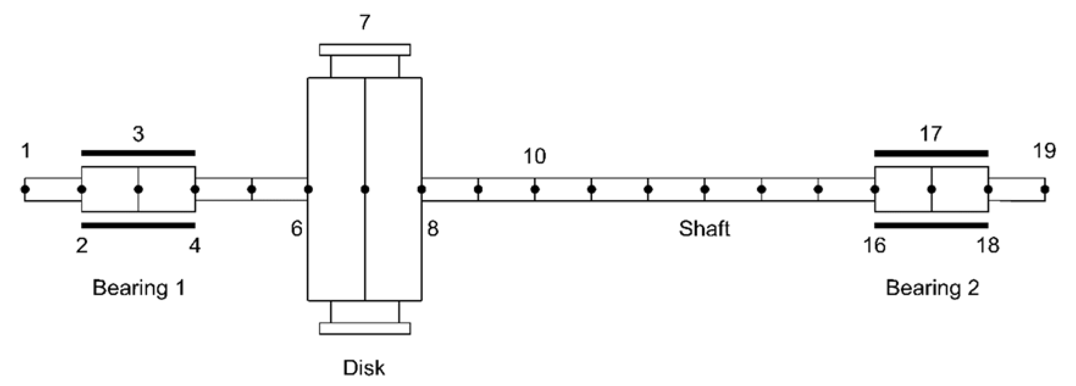
The rotating system used is shown in Figure 2. It consists of 18 beam elements (19 nodes) and 1 disk element. The SAE 1020 steel shaft has elastic modulus of 2 × 10¹¹ N/m², poison coefficient of 0.3, 7800 kg/m³ density, 700 mm length, 15 mm diameter. Moreover, it is supported by two hydrodynamic bearings, placed approximately at 580 mm from each other, positioned at nodes 3 and 17, respectively, having a length of 20 mm, an inner diameter of 31 mm with 90 μm of radial clearance. The lubricant is the ISO VG 32 oil at a constant average temperature of 40 °C ($\mu$ = 2.7622 × 10⁻² Pa·s). The disk was placed at node 7, positioned 200 mm from bearing 1, with 94.7 mm diameter and 47 mm length. In this case, the unbalanced mass was $m_0=3$ g, located 37 mm away from the center of the disk. In addition to the unbalance, a 200 N external force was applied to the disk node to simulate a severe loading condition. As shown in Equation (12), the structural damping can be proportional to the mass and stiffness matrices, but for steel shafts, the recommendation is to only use a matrix proportional to the stiffness. Therefore, the coefficients used here were $\alpha =0 \mathrm{and} \beta =1.5\times {10}^{-5}$ (this value was experimentally estimated in [17]).

Is worth noting that the procedures used for the simulations—the finite element modelling and time integration scheme, as well as the solution of the Reynolds equation—have been experimentally validated in [17] for a rotor system supported by cylindrical journal bearings. Although the bearing geometries presented are different from the cylindrical one, the procedure used to solve the Reynolds equation is the same of [17].

Figure 3 shows the pressure field distribution in each bearing (elliptical and trilobed) in order to exemplify its behavior in each analyzed geometry. Preload 0.8 was used, since the pressure peaks can be better visualized in this situation. When considering the elliptical bearing, it is possible to observe the presence of two pressure peaks due to the two lobes. Similarly, for the three-lobe bearing, three pressure peaks are seen due to the three lobes.

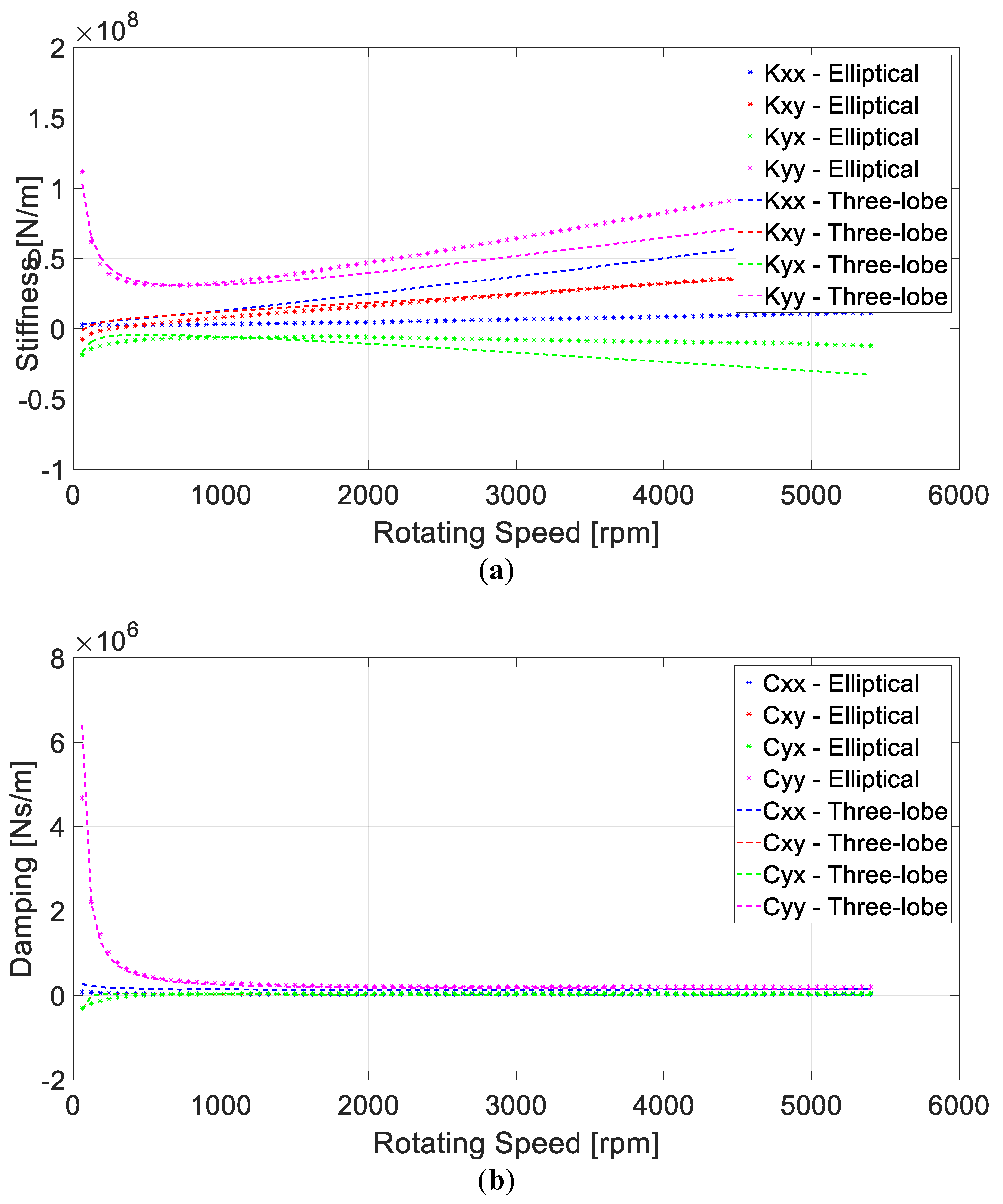
Figure 4 depicts the behavior of the stiffness (Figure 4a) and damping (Figure 4b) coefficients for the elliptical and three-lobe bearings, which are a function of the rotating speed. These coefficients are used in the linear bearing approach. Analyzing the dynamic coefficients, it is possible to note that the cross-coupled coefficients (xy, yx) for the three-lobe case are smaller than for the elliptical case, confirming that three-lobe bearings present greater stability in comparison to the elliptical one, as expected.

3.1. Numerical Results of Orbits

The numerical analyses made here compare the orbits of shaft inside the bearings. Since the rotor is asymmetric to the presence of a decentralized disk, as seen in Figure 2, bearing 1 was chosen for viewing the orbits, since gyroscopic effects are more evident there. The first critical speed of the system is about 37 Hz. Thus, five rotating speeds were selected to evaluate the orbit behavior in conditions of high eccentricity (below first critical speed), low eccentricity (above first critical speed) and high amplitudes (around first critical speed) being 15, 30, 35, 45 and 60 Hz. Additionally, the Sommerfeld number range goes from 0.049 to 0.2.

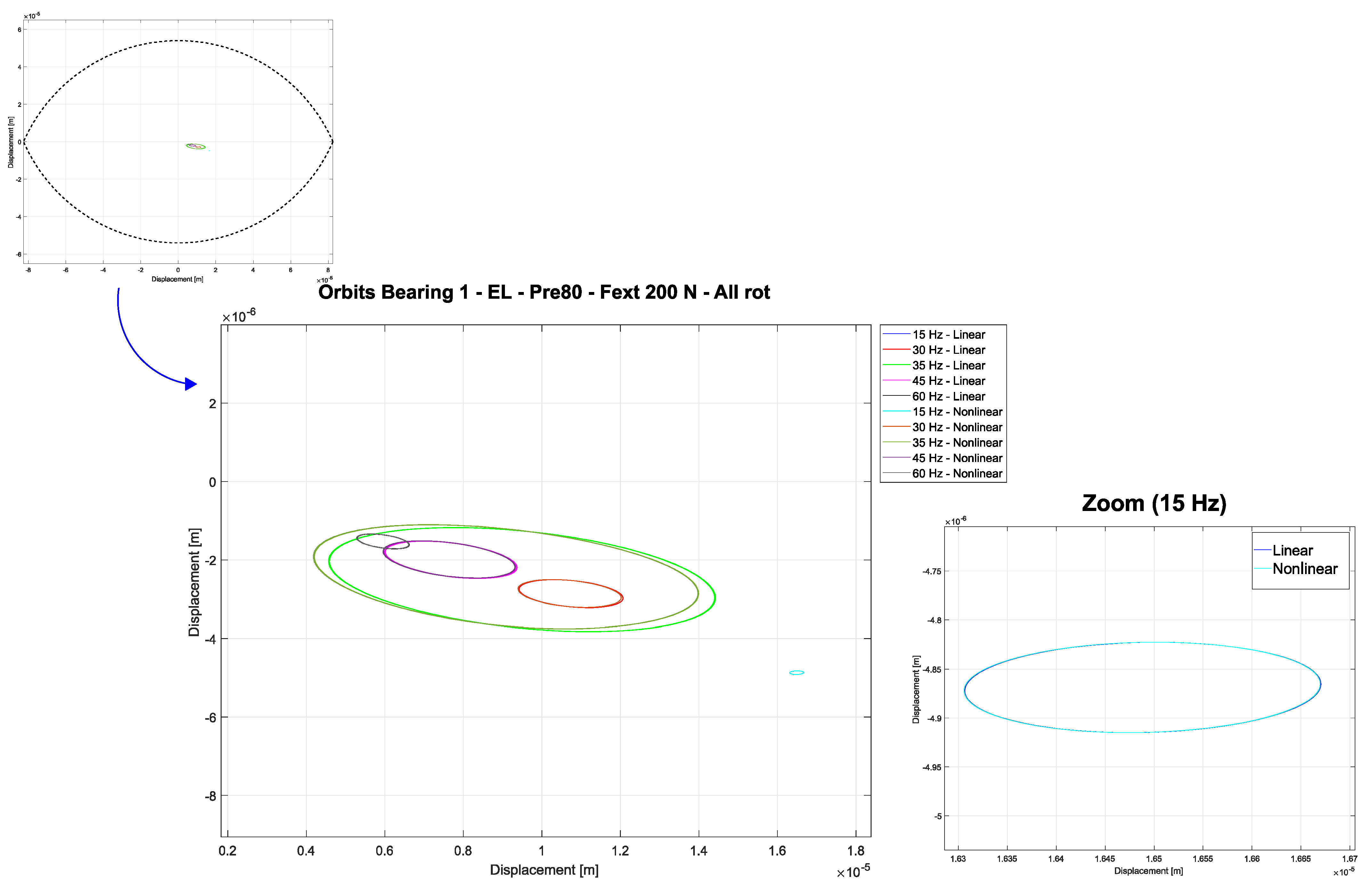
Figure 5 shows the orbits results for the elliptical bearing with preload of 0.25. A total simulated time of 20 s is used, in which only the last second of the converged orbit is plotted. It is possible to visualize the “self-centering” effect, in which with increasing rotating speed the shaft tends to be centered in the radial clearance of the bearing. Additionally, the major discrepancies between linear and nonlinear models occur near the first critical speed of the system (35 Hz, green lines), where the vibration amplitude is higher. In this case, either shape or size can be different when considering the nonlinear model. For the other rotating frequencies, just slight differences can be observed between the models, maintaining similar orbit shapes and positions.

By increasing the preload level to 0.8, the shapes of the orbits remained similar, except for 35 Hz, which has differences due to the proximity with the critical speed (Figure 6). However, the orbits are smaller than the previous case, since the higher the preload, the smaller the radial clearance in the vertical direction, which creates a stiffer oil film and, consequently, reduces the vibration amplitudes. Additionally, it is interesting to note that Figure 6 shows a zoom in the whole region containing the orbits.

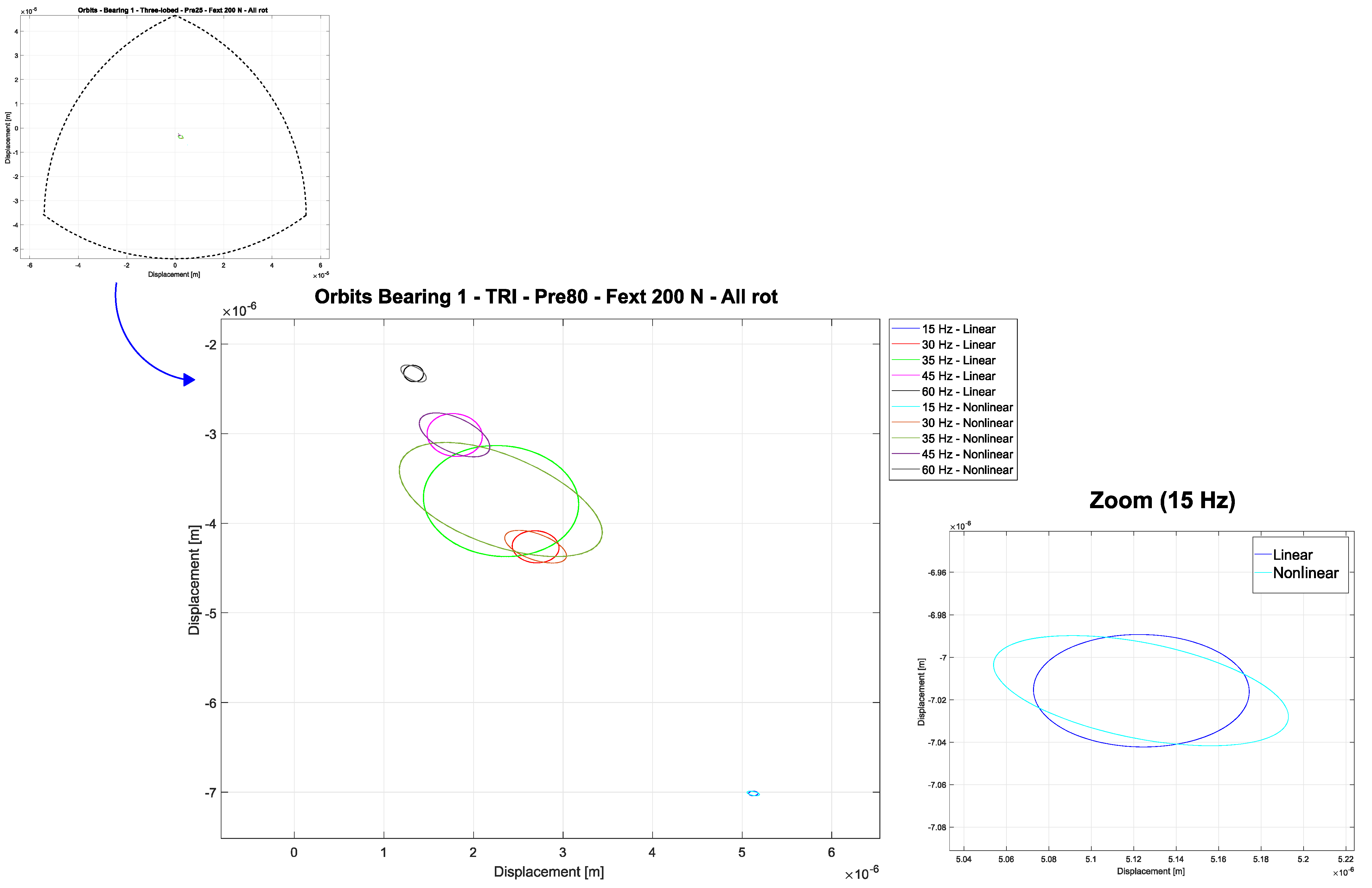
Changing the bearing type, Figure 7 shows orbits for the three-lobed bearing with preload 0.25. In this case, differences in size can be observed at all rotating speeds, indicating a greater influence of nonlinearities in this bearing geometry. At 35 Hz, near the first critical speed, the discrepancies in size are ever higher, and it is possible to observe differences in shape and position as well.

For the three-lobed bearing with preload 0.8, the central position of the orbits remained the same for all rotating speeds (comparing linear and nonlinear approaches), as shown in Figure 8. However, the orbits’ size and shape change at all rotations in an evident way. In the proximity of the critical region (35 Hz), the amplitude of the orbit increases, but as stated, maintaining the same position. This shows that the nonlinearity substantially affects three-lobed bearings and has an even greater effect in the case of high preload.

According to results obtained by the calculation of the orbits, the conclusion is that for elliptical bearings the nonlinearities are only influential in cases of higher orbit amplitudes, i.e., in the vicinity of the critical speed. This behavior is similar to that observed in cylindrical bearings, as shown in the work of reference [17]. On the other hand, in the case of three-lobed bearings, the influence of nonlinearities is much more evident, being practically observed in all rotating speeds, with greater sensitivity the higher the value of the bearing preload.

3.2. Numerical Results of DFT Full Spectrum

Spectral analysis is an alternative way of identifying and analyzing signals, which becomes complementary to time domain analysis. For this, the signal is decomposed in the frequency domain, allowing the identification of the components of that signal. A known tool for the treatment of discrete and aperiodic signals is the DFT (“Discrete Fourier Transform”). A conventional DFT is called a “half spectrum”, as it relates only the positive part of the frequency domain, commonly in harmonics, e.g., 1×, 2×, 3× etc. For cases in which information about the relative phase is important, such as in the diagnosis of unbalance and misalignment faults, among others, the application of the “DFT full spectrum” is indicated [27]. In these situations, the full spectrum enables the determination of the rotor’s behavior under “forward” and “backward” precession conditions.

Each orbit has, in general, an elliptical shape, which can be represented as the sum of two circular orbits, one in forward rotation and the other in backward rotation, both rotating at the same frequency, which is the frequency of the filtered orbit. Thus, the orbit will be more or less circular, depending on the amplitude of the signal components in the frequency domain.

Therefore, Figure 9 shows the first results for the elliptical bearing 1, with preload 0.25, using the DFT full spectrum decomposition. To facilitate the interpretation of the graphs,

Table 1. Magnitudes of the most relevant peaks of Figure 9—elliptical bearing (preload 0.25).

Rot. Speed	Amplitudes (m)
	Linear						Nonlinear
	−3×	−2×	−1×	1×	2×	3×	−3×	−2×	−1×	1×	2×	3×
15 Hz	-	-	1.27 × 10−7	2.04 × 10−7	-	-	-	-	1.46 × 10−7	2.36 × 10−7	-	-
30 Hz	-	-	1.31 × 10−6	2.44 × 10−6	-	-	-	6.94 × 10−8	1.39 × 10−6	2.62 × 10−6	7.41 × 10−8	-
35 Hz	-	-	6.67 × 10−6	1.27 × 10−5	-	-	2.30 × 10−7	1.11 × 10−6	5.32 × 10−6	1.11 × 10−5	1.24 × 10−6	1.78 × 10−7
45 Hz	-	-	1.89 × 10−6	3.97 × 10−6	-	-	-	1.26 × 10−7	1.85 × 10−6	3.93 × 10−6	1.26 × 10−7	-
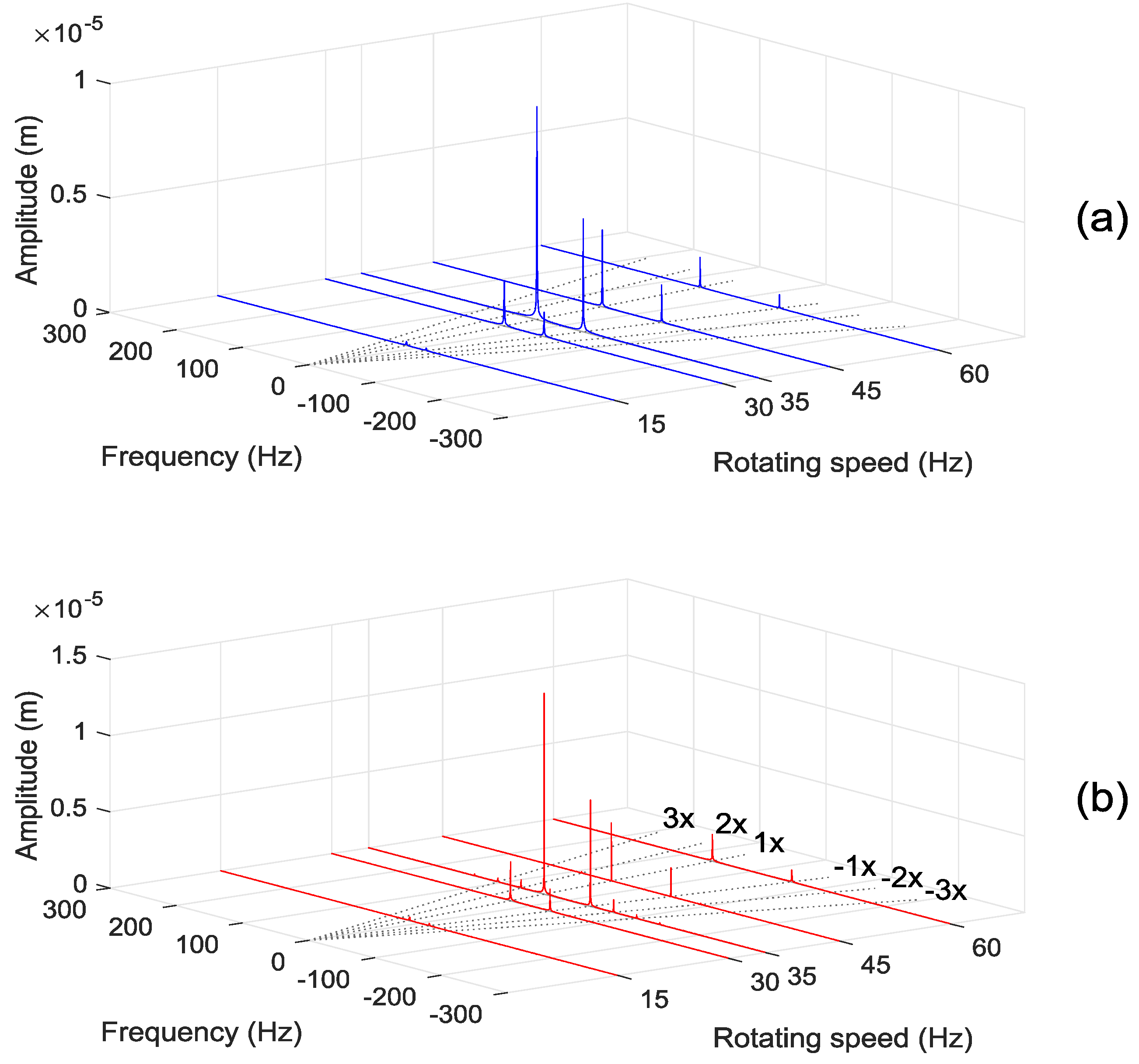
60 Hz	-	-	6.07 × 10−7	1.39 × 10−6	-	-	-	2.06 × 10−8	7.19 × 10−7	1.65 × 10−6	2.30 × 10−8	-

brings a comparison of the magnitudes of the most relevant amplitude peaks for all analyzed cases. The intention is to compare the influence of linear and nonlinear models on the frequency spectrum for the different bearing types.

It is possible to observe the presence of the −1× component in all rotations, for both models, on the left-hand side of the spectrum, i.e., frequency related to backward mode, due to the fact that hydrodynamic bearings inherently introduce some anisotropy into the system. In linear cases, there are only the 1× and −1× components, indicating the purely elliptical shape of the orbit, as can be attested in Figure 5. For nonlinear cases, there are significant values related to high order harmonics, such as 2× and −2×. For 35 Hz, the components −3× and 3× appear, indicating the proximity of the system’s critical speed region, which is an indication that the system is more nonlinear under these conditions. These additional harmonics influences the orbit size and shape, which can again be clearly observed in Figure 5.

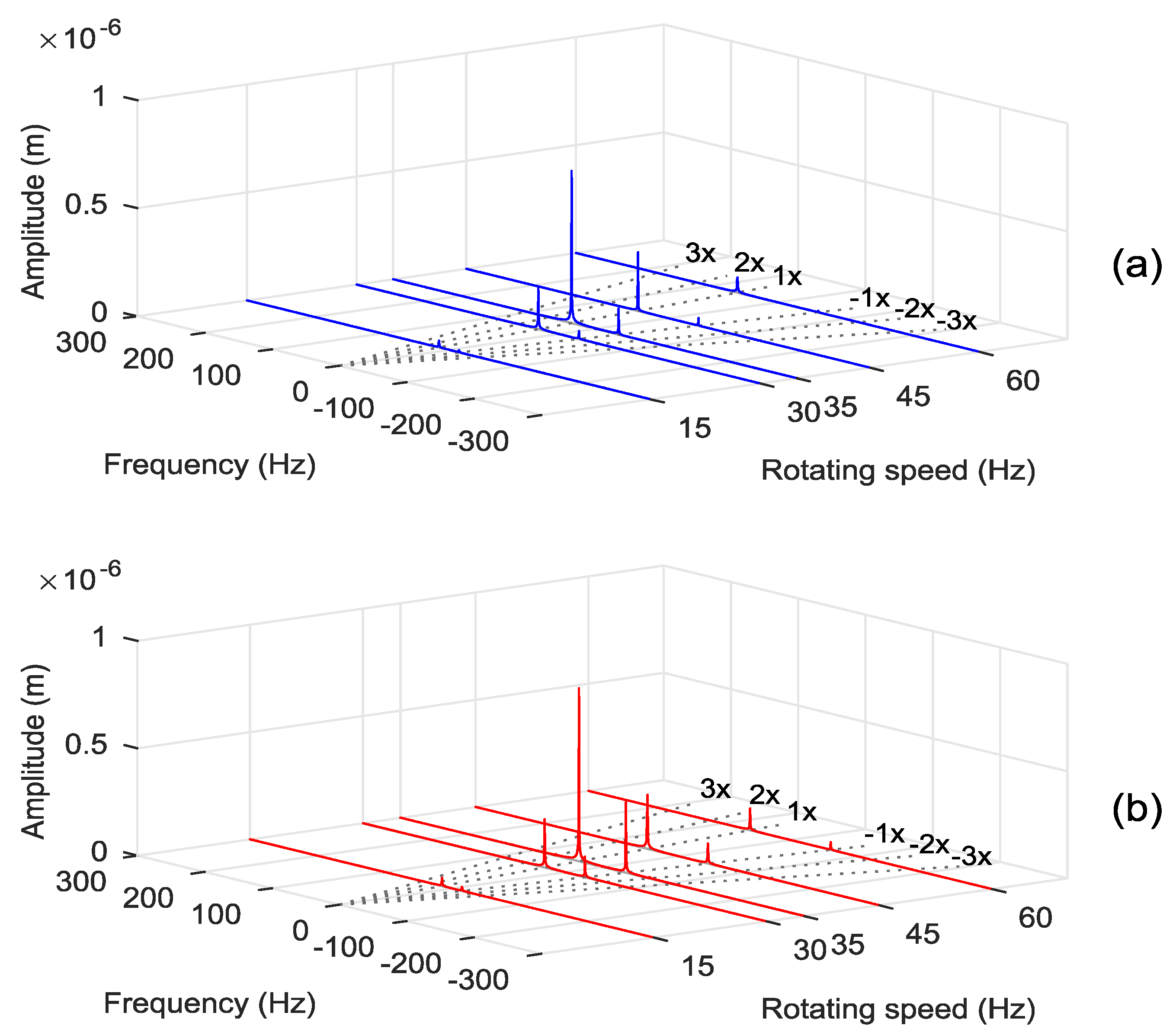
By increasing the preload to 0.8, for the elliptical bearing 1, it is possible to observe similar behavior to the case of smaller preload, as shown in Figure 10 and

Table 2. Magnitudes of the most relevant peaks of Figure 10—elliptical bearing (preload 0.8).

Rot. Speed	Amplitudes (m)
	Linear						Nonlinear
	−3×	−2×	−1×	1×	2×	3×	−3×	−2×	−1×	1×	2×	3×
15 Hz	-	-	5.42 × 10−8	9.07 × 10−8	-	-	-	-	5.46 × 10−8	9.10 × 10−8	-	-
30 Hz	-	-	4.42 × 10−7	7.38 × 10−7	-	-	-	1.00 × 10−8	3.93 × 10−7	6.56 × 10−7	1.34 × 10−8	-
35 Hz	-	-	1.77 × 10−6	2.94 × 10−6	-	-	-	7.58 × 10−8	1.85 × 10−6	3.08 × 10−6	1.25 × 10−7	-
45 Hz	-	-	6.28 × 10−7	1.05 × 10−6	-	-	-	7.08 × 10−9	6.32 × 10−7	1.06 × 10−6	1.14 × 10−8	-
60 Hz	-	-	1.74 × 10−7	2.89 × 10−7	-	-	-	-	2.53 × 10−7	4.19 × 10−7	-	-

. The amplitudes are at least 1 order of magnitude lower, and there is no presence of −3× and 3× components for the rotation of 35 Hz, due to the smaller orbit originated by the low journal eccentricity.

For the three-lobed bearing 1, with preload 0.25, it is possible to see in Figure 11 and

Table 3. Magnitudes of the most relevant peaks of Figure 11—three-lobed bearing (preload 0.25).

Rot. Speed	Amplitudes (m)
	Linear						Nonlinear
	−3×	−2×	−1×	1×	2×	3×	−3×	−2×	−1×	1×	2×	3×
15 Hz	-	-	1.10 × 10−7	1.74 × 10−7	-	-	-	-	1.42 × 10−7	2.17 × 10−7	-	-
30 Hz	-	-	1.07 × 10−6	1.96 × 10−6	-	-	-	4.12 × 10−8	1.44 × 10−6	2.55 × 10−6	3.97 × 10−8	-
35 Hz	-	-	4.94 × 10−6	9.31 × 10−6	-	-	2.43 × 10−7	8.27 × 10−7	6.97 × 10−6	4.32 × 10−5	5.23 × 10−7	2.54 × 10−7
45 Hz	-	-	1.64 × 10−6	3.36 × 10−6	-	-	-	8.38 × 10−8	1.87 × 10−6	3.80 × 10−6	7.54 × 10−8	-
60 Hz	-	-	5.83 × 10−7	1.31 × 10−6	-	-	-	-	7.84 × 10−7	1.73 × 10−6	-	-

that amplitudes 1× and −1× are greater for the nonlinear case (mainly the forward component 1×). Higher vibration orbits are more prone to nonlinearities coming from the hydrodynamic bearings. So, it is possible to state that the three-lobed bearing is more susceptible to present nonlinear behavior, as can also be seen by the presence of additional harmonics in the signal. Comparing Table 1 and Table 3, it is perceivable that these differences are higher for the three-lobed bearing. Regarding the other harmonic components for all rotations, they have similar behavior to those observed for the elliptical bearing cases.

Finally, Figure 12 and

Table 4. Magnitudes of the most relevant peaks of Figure 12—three-lobed bearing (preload 0.8).

Rot. Speed	Amplitudes (m)
	Linear						Nonlinear
	−3×	−2×	−1×	1×	2×	3×	−3×	−2×	−1×	1×	2×	3×
15 Hz	-	-	9.82 × 10−9	3.08 × 10−8	-	-	-	-	1.96 × 10−8	3.84 × 10−8	-	-
30 Hz	-	-	3.73 × 10−8	1.95 × 10−7	-	-	-	-	9.50 × 10−8	2.24 × 10−7	-	-
35 Hz	-	-	1.20 × 10−7	7.04 × 10−7	-	-	-	-	3.29 × 10−7	8.06 × 10−7	-	-
45 Hz	-	-	3.57 × 10−8	2.71 × 10−7	-	-	-	-	9.36 × 10−8	2.52 × 10−7	-	-
60 Hz	-	-	6.83 × 10−9	6.99 × 10−8	-	-	-	-	3.56 × 10−8	1.02 × 10−7	-	-

show the results for the three-lobed bearing 1 with preload 0.8. This case has somewhat different behavior. The only frequency components observed are 1× and −1×, indicating a purely elliptical shape of the orbit for both linear and nonlinear models, even though the orbits obtained with the two models are quite different, as shown in Figure 8. By observing the rotating speeds and comparing the models, it can be seen that the 1× amplitudes have very close values, with just slight differences. However, the nonlinear −1× amplitudes have higher values when compared to the linear ones, indicating the deformations in the orbits (Figure 8), which means more anisotropy in the system, since in this case, the backward component is greater.

Analyzing the decomposition of the signals by DFTs, it is possible to conclude that, for low preloaded bearings, for both elliptical and three-lobed cases, the nonlinearities are more detectable through the appearance of higher order harmonics, such as 2×, 3× (forward) and −2×, −3× (backward). On the other hand, for the case of three-lobed bearings with high preload, the nonlinearities are evidenced by the increased growth in the backward component −1×.

4. Conclusions

The paper presents comparative results of linear and nonlinear models for elliptical and three-lobe hydrodynamic bearings, operating under severe loading conditions. The analysis included the comparison of the orbits (by the numerical integration of the system in time-domain) and signal amplitudes in the frequency domain (by DFT full spectrum).

Regarding the presented orbits, the results showed that for elliptical bearings, the situations with the greatest presence of nonlinearities occur with high vibration amplitudes, near the critical speed region, whereas for three-lobed bearings, the nonlinearities have greater influence even in smaller vibration amplitude situations.

An important point was seen in the analysis of the full spectrum, which showed that nonlinearities are not always evidenced by the appearance of higher order harmonic components but can also be presented through a significant increase in the −1× component.

Finally, the combined analyses presented here are of great importance for mapping the influence of nonlinearities in different types of multi-lobed hydrodynamic bearings with fixed geometry. As the number of lobes, and/or the preload value, increases, the vibration levels decrease, generally pointing to a more linear bearing. Consequently, the traditional linear analysis could be employed without major drawbacks. This study is important for monitoring and fault diagnosis, mainly those that are model based since representative mathematical models are mandatory for a reliable diagnosis.