Article

Predictive Maintenance for Remanufacturing Based on Hybrid-Driven Remaining Useful Life Prediction

1
College of Engineering and Physical Sciences, Aston University, Birmingham B4 7ET, UK
2
Harms & Wende GmbH & Co. KG, 21079 Hamburg, Germany
3
Information Technologies Institute, Center for Research and Technology Hellas, 57001 Thessaloniki, Greece
*
Authors to whom correspondence should be addressed.
Appl. Sci. 2022, 12(7), 3218; https://doi.org/10.3390/app12073218
Submission received: 23 February 2022 / Revised: 20 March 2022 / Accepted: 20 March 2022 / Published: 22 March 2022
(This article belongs to the Special Issue Manufacturing Sustainability in a Circular Economy)

Abstract

:
Remanufacturing is an activity of the circular economy model whose purpose is to keep the high value of products and materials. As opposed to the currently employed linear economic model, remanufacturing targets the extension of products and reduces the unnecessary and wasteful use of resources. Remanufacturing, along with health status monitoring, constitutes a key element for lifetime extension and reuse of large industrial equipment. The major challenge is to determine if a machine is worth remanufacturing and when is the optimal time to perform remanufacturing. The present work proposes a new predictive maintenance framework for the remanufacturing process based on a combination of remaining useful life prediction and condition monitoring methods. A hybrid-driven approach was used to combine the advantages of the knowledge model and historical data. The proposed method has been verified on the realistic run-to-failure rolling bearing degradation dataset. The experimental results combined with visualization analysis have proven the effectiveness of the proposed method.

1. Introduction

Modern manufacturing is the critical component in the circular economy (CS). However, the unsustainable development methods of modern manufacturing are continually causing environmental problems [1]. In recent years, carbon neutrality has been proposed as a common interest of the world. As one of the biggest carbon emitters, the manufacturing industry should eagerly transfer the current operating mode to more sustainable processes [2,3]. Although production decisions and carbon regulations have been studied, more actions are needed to implement sustainable manufacturing [4]. As an alternative to the traditional linear economy, the circular economy has obtained more attention from industry partners. Nowadays, policy makers and scholars are focused on waste prevention and the improvement of resource efficiency, which aims to decrease waste by reducing the use of new raw materials [5,6,7].
Remanufacturing is a sustainability option of the material circular economy [8]. Compared to traditional strategies in the CE, such as recycling, reuse and refurbishment, remanufacturing is an advanced solution. Recycling takes the raw material of wasted products to create new parts. Reuse directly uses the available components in new products. Refurbishment is designed to repair and restore the failed products to a new state, which should have a shorter warranty than the new product. This makes the strategy difficult to implement on complex machines [9,10]. Remanufacturing is a life-extension method that would use a combination of reused and repaired components to rebuild the as-good-as-new conditioned manufactured product. The main process includes disassembly, cleaning, inspection, repairing and replacing parts and reassembly. It not only saves the cost of manufacturing, but also reduces the consumption of energy and materials. Remanufacturing could save up to 80% of the cost and 85% of the energy of using new components [11,12]. Although remanufactured products have been used in several industrial sectors, when and how remanufacturing should be conducted is still a challenge facing manufacturers [13].
For remanufacturing, there is an ideal high remanufacturability zone that has the optimal remanufacturability and its cost [14]. The remanufacturability is a criterion for the component of future remanufacturing [15,16]. It considers the following factors: the quality of the component before remanufacturing, the importance of the component, the technology used for remanufacturing, and the customer awareness of component remanufacturing. These factors were considered in the proposed method to thoroughly assess the remanufacturability of the component. For a new component, reliability is an important factor for assessing degradation and indicating quality.
As the component deteriorates over time, the remaining useful life becomes shorter while the reliability of the component decreases. If the reliability is below the lower threshold of the ‘high remanufacturability zone’, the remanufacturability of the components will not be sufficient, and the cost of remanufacturing will become too high. As shown in Figure 1, preventive maintenance can help maintain the remaining useful life (RUL) of components within the high remanufacturability zone. In the left figure, the yellow line indicates service time with maintenance. Maintenance actions are carried out according to the level of reliability during this period. Each time after the maintenance, reliability becomes higher than before, and the remanufacturability remains in a high zone. Accordingly, as shown in the right figure, the cost of remanufacturing, the remanufacturability and the value of the equipment are changing along the time dimension. In the ‘high remanufacturability zone’, the remanufacturability is kept high, while the cost of remanufacturing is relatively low, and the value of the equipment is still acceptable. Therefore, it is worth noting that predictive maintenance could support remanufacturing very effectively, allowing experts to make the optimal decision in such a framework.
Predictive maintenance (PdM) is designed for evaluating the state of the in-service machine and generating a plan for when maintenance should be performed [17]. It is considered condition-based maintenance which is based on the estimated performance of degradation of the equipment. Different from traditional preventive maintenance, PdM is capable of dynamically predicting when maintenance will be needed rather than relying on the static average or expected life statistics. Moreover, some studies show that PdM could help improve remanufacturability and reduce the remanufacturing cost [18].
With the development of industrial 4.0, the PdM techniques have been widely applied to many real-world industrial applications combined with historic data, models, and domain knowledge [19]. For complex equipment, condition monitoring (CM) is the most effective way to evaluate performance based on practical data [20]. The traditional CM methods extract the effective features from the original data, then build a health index to identify the condition of the machine [21,22,23]. The intelligent CM methods aim at directly assessing the state of the machine from the data, which have been made available with the rapid development of machine learning techniques [24,25,26,27].
As the most critical part of predictive maintenance, remaining useful life predictions are designed to estimate the future state of a component based on current and historical data [28,29]. Data collection and processing and condition monitoring are the foundation for supporting the PdM. Dynamic maintenance scheduling can only work after acquiring the prediction of future states. Generally, there are three types of methods to carry out RUL prediction, including model-based, data-based, and hybrid-based approaches [30,31,32]. Model-based methods use the physical model of the degradation process, which is extracted from the expert knowledge about the life cycle of a given product. The main algorithms to implement the model-based approaches are particle filtering [33,34] and its variants [35]. However, an accurate knowledge model could barely be derived for complex equipment. In contrast, data-based methods do not rely on knowledge of the degradation process but will learn the model relationship from data. Machine learning methods are used to learn the degradation prediction functions, mainly including general neural network [36], convolution neural network [37] and recurrent neural network [38]. Nevertheless, these approaches do not match the requirement of the dynamic degradation process; when new data have been collected, they need massive time to retrain the model. The principle motivation for this paper is to use the hybrid-based approach, which utilizes both model-based and data-based approaches for developing a predictive maintenance framework for remanufacturability.
The proposed method and detailed specifications are described in Section 2. Section 3 shows detailed experiments and analysis results. The conclusions are included in Section 4.

2. Proposed Methodology

This paper presents an innovative combination of model-based and data-based approaches resulting in an effective predictive maintenance framework for remanufacturability. The proposed PdM framework mainly employs three modules; condition monitoring, remaining useful life prediction, and dynamic maintenance scheduling, as shown in Figure 2, to keep the equipment well-functioning, increase its availability, and support the expert to make the right decision regarding the optimal period to move the machine or the critical component to remanufacturing. A detailed description of the PdM framework is presented next.

2.1. Condition Monitoring

Condition monitoring is regarded as a pivotal component of the proposed predictive maintenance framework. It aims to inspect and evaluate the current state of a machine or its components through the original real-time data collected from different types of sensors (e.g., vibration, noise, temperature, etc.) connected to the machine [39]. The advanced predictive maintenance framework is built on the condition monitoring system, then integrates effective prognostic approaches that can estimate the future condition [40,41]. In this work, the CM module consists of the following two tasks: feature extraction and performance assessment.

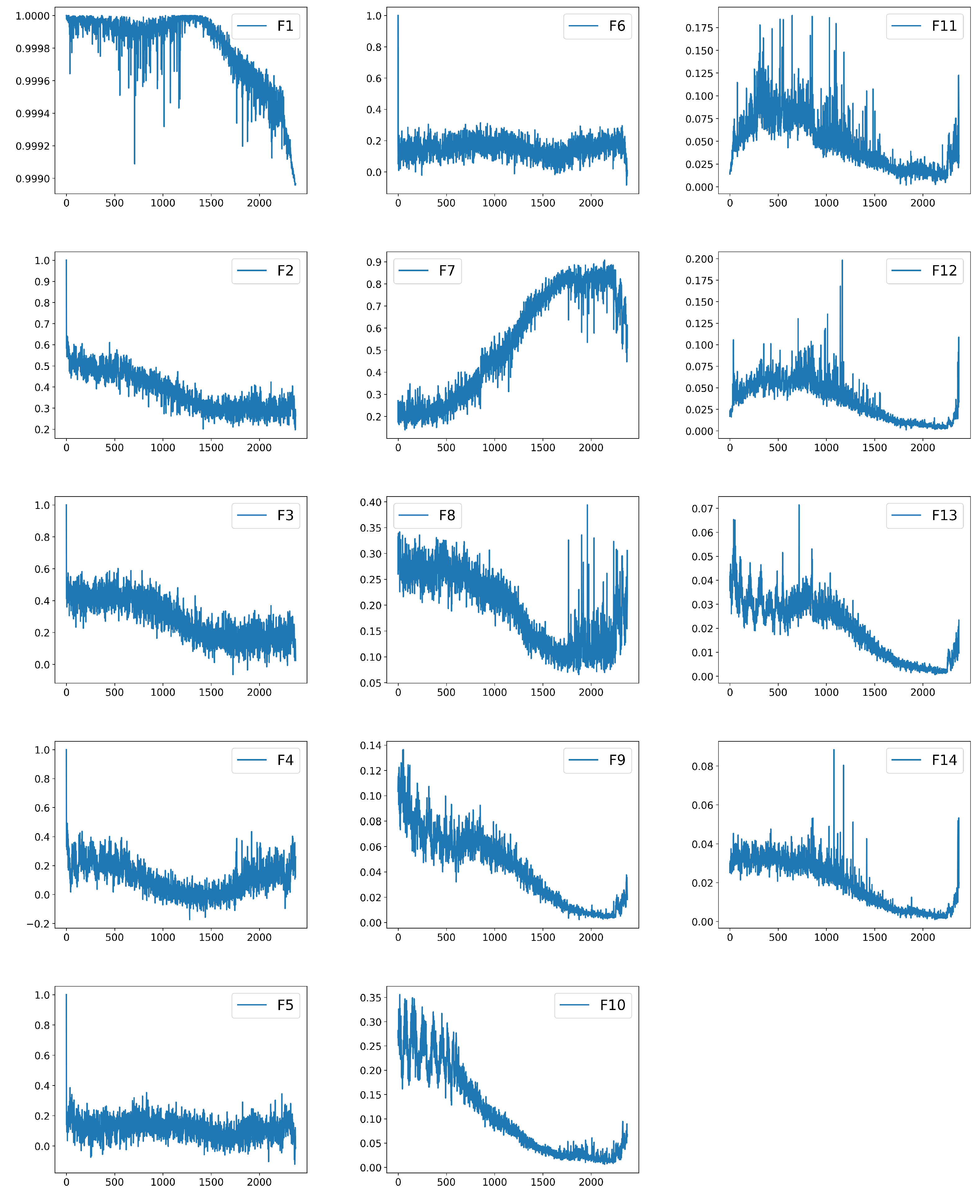
2.1.1. Feature Extraction

The purpose of feature extraction is to acquire more reasonable feature information that could improve the accuracy of performance assessment compared with the original signal. In this work, the vibration signal is used as the original information; then we select the feature extraction method based on the research [38]. These features are studied and proven to be monotonically related to the whole degradation procedure. The details of the features set is shown in Table 1.
As shown in Table 1, there are 14 features, six of them are related-similarity (RS) features including one time-domain RS feature and five frequency-domain RS features. The RS feature represents the similarity between the current features and the benchmark data, which are expressed as follows:
R S t = | i = 1 k ( f 0 i f ¯ 0 ) ( f t i f ¯ t ) | i = 1 k ( f 0 i f ¯ 0 ) 2 i = 1 k ( f t i f ¯ t ) 2
where f t is the features of current data, f 0 is the feature from the initial time, k is the number of features, f ¯ 0 and f ¯ t are the mean value of their features, respectively.
For the first time-domain RS feature, there are 11 traditional features, including mean, RMS, kurtosis, skewness, peak-to-peak, variance, entropy, crest factor, wave factor, impulse factor, and margin factor. The frequency-domain features are extracted from the FFT (fast Fourier transform) spectrum so that the features of the whole spectrum and four subset spectrum are produced. F7 to F14 are time-frequency-domain features, which are extracted from the outcome of WP (wavelet package) transform at the three-level decomposition.

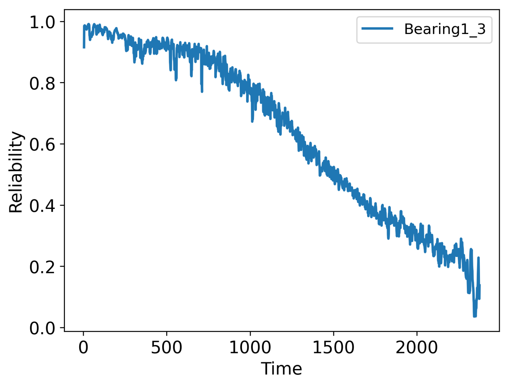
2.1.2. Performance Assessment

Although the feature extraction has already obtained very useful information, the expert may not be able to understand the real-time condition because many features still need to be known at each time step. Therefore, the performance assessment task is designed to combine the features into a single health index that represents the condition of the equipment. In order to assess the condition of the whole run-to-failure degradation process, the Pearson correlation coefficient (PCC) was selected to compute degradation performance. It has been verified as a reasonable evaluation method for vibration data [42]. Generally, the PCC is decreasing with the state degradation. Details of how PCC is calculated are given below:
  • The first step is normalizaing the extracted features:
    x t = x t x m i n x m a x X m i n
    where x t is the feature at the time t, which will be normalize into [0, 1].
  • The second step is to calculate the PCC with the obtained features between normal state and the real-time state:
    PCC ( x , y ) = i = 1 n ( x i x ¯ ) ( y i y ¯ ) i = 1 M ( x i x ¯ ) 2 i = 1 n ( y i y ¯ )
    where x and y are two different feature vectors and n is the length of a feature vector.

2.2. Prognositc Approach: Hybrid-Driven Remaining Useful Life Prediciton

The prognostic module is designed to estimate the future state based on current state and historical data. This is calculated through predicting the remaining useful lifetime using both the knowledge-based degradation model and the data-driven optimization approach. Such a hybrid-driven approach enables predicting the RUL without the need for a large amount of data.

2.2.1. Knowledge-Based Degradation Model

As one of the most popularly used lifetime degradation distribution models, the Weibull distribution has been widely studied in many real-world applications [43,44,45]. It is a versatile distribution with two parameter η and β that could fit the reasonable distribution in reliabilityengineering.
The PDF (probability density function) of Weibull distribution is defined as:
f ( t ) = β η t η β 1 e t η β
The Weibull CDF (cumulative density function) is defined as:
F ( t ) = 1 e ( t η ) β
Based on Equations (4) and (5), the reliability function (also regarded as, survival function) can be defined as below:
R ( t ) = e ( t η ) β
Equation (6) is the predefined degradation model, which is the probability to survive of a component with t denoting usage time of the component and β and η are the Weibull parameters. The shape parameter β is generally considered β 1 , and it describes the aging process of components over time. The case of β = 1 corresponds to process or Weibull degradation where the component never gets old. If such a component survived an arbitrarily long time t its remaining expected lifetime is determined solely by η (independent of t).

2.2.2. Model Parameter Identification

The proposed Weibull distribution model is considered as measuring the reliability of the equipment. Once the two parameters η and β are determined, we can obtain the whole degradation process in terms of the period. A nonlinear least-square method [46] was selected in the proposed predictive maintenance framework to learn the reliability model parameters using both historical data and the current state information obtained from the condition monitoring module. The mathematical formulation for optimizing the reliability model parameters is expressed as follows:
arg min η , β t = 0 T y t e ( t η ) β 2
where y t is the historical reliability at t, T is the current time.

2.2.3. Remaining Useful Lifetime Calculation

The future degradation states could be estimated by the learned reliability function at the inspection time T. The equipment should be shut down when the reliability is close to the specific threshold. Therefore, the RUL can be defined as:
RUL ( T ) = i n f { r : R ( r + T ) ω | R }
where RUL ( T ) is the RUL at T, R ( r + T ) is the estimated reliability at r + T , and ω is the failure threshold.

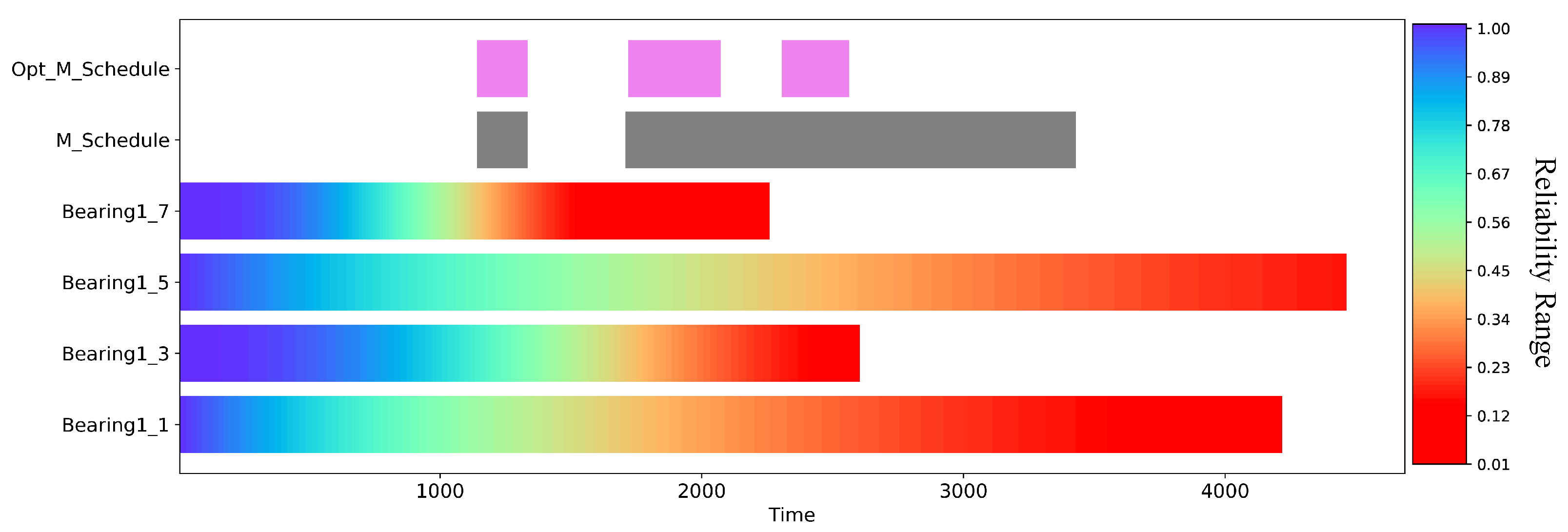
2.3. Dynamic Maintenance Scheduling

Dynamic maintenance scheduling (DMS) provides the company with the optimized period to conduct maintenance strategies, which could implement dynamic searching for the optimal maintenance duration with the help of prognostic approaches [47]. This will provide the stakeholder more of a chance to benefit by increasing the availability of the machine while it continues to well-function. Meanwhile, the machine and its key component could be replaced at the optimal time to be remanufactured so that its life cycle is extended. The overall workflow of the proposed framework is shown in Figure 3, which obviously displays the relationship between the DMS, CM, and RUL module. The experts could make comprehensive decisions following the optimal maintenance period so that the company will obtain more business benefits.

3. Experiment and Result

The proposed PdM method has been tested on the run-to-failure rolling bearing degradation dataset, which come from the IEEE PHM Challenge [48]. The data have been collected on the PRONOSTIA testbed, and accelerated degradation experiments have been carried out.

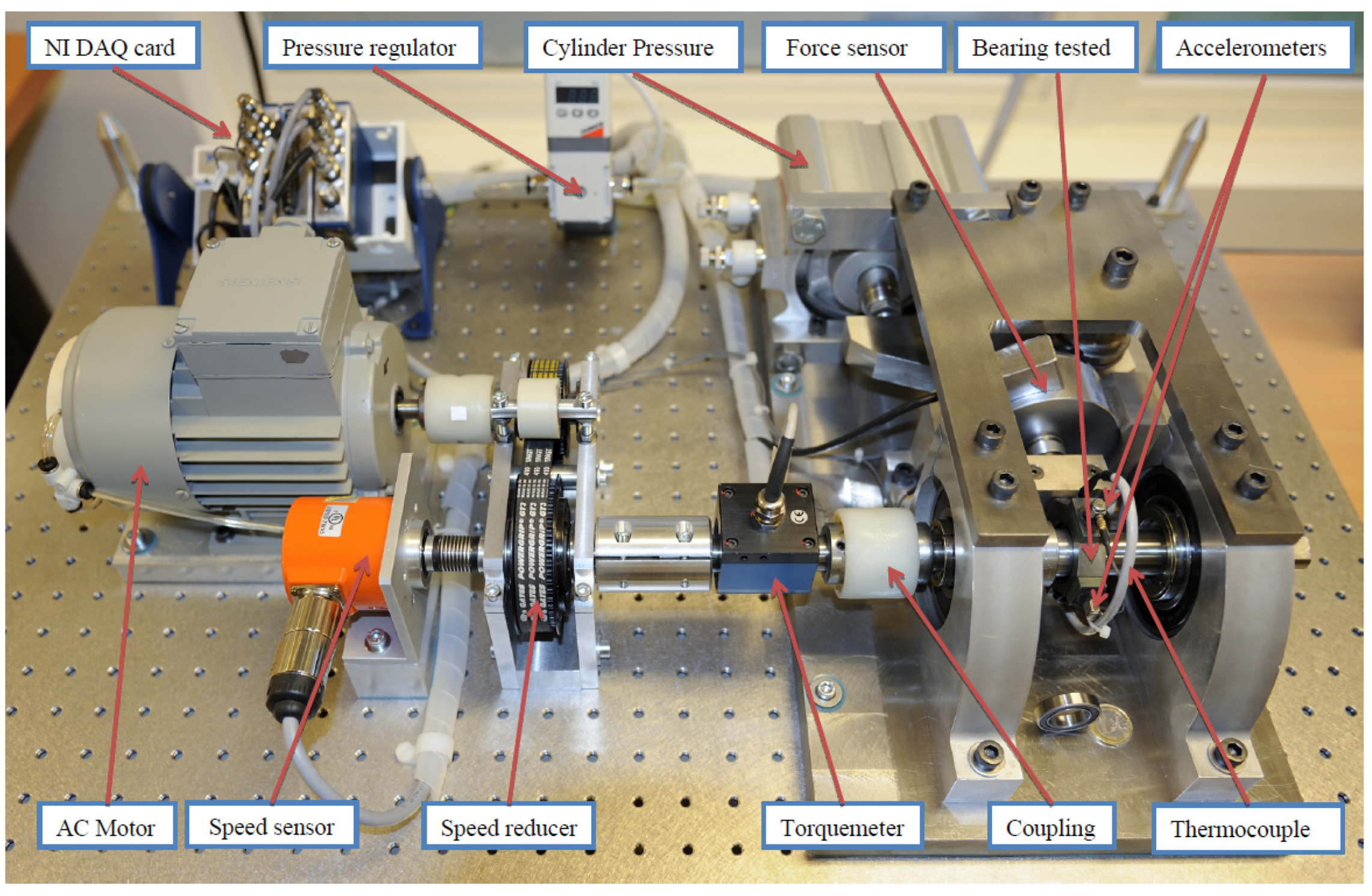
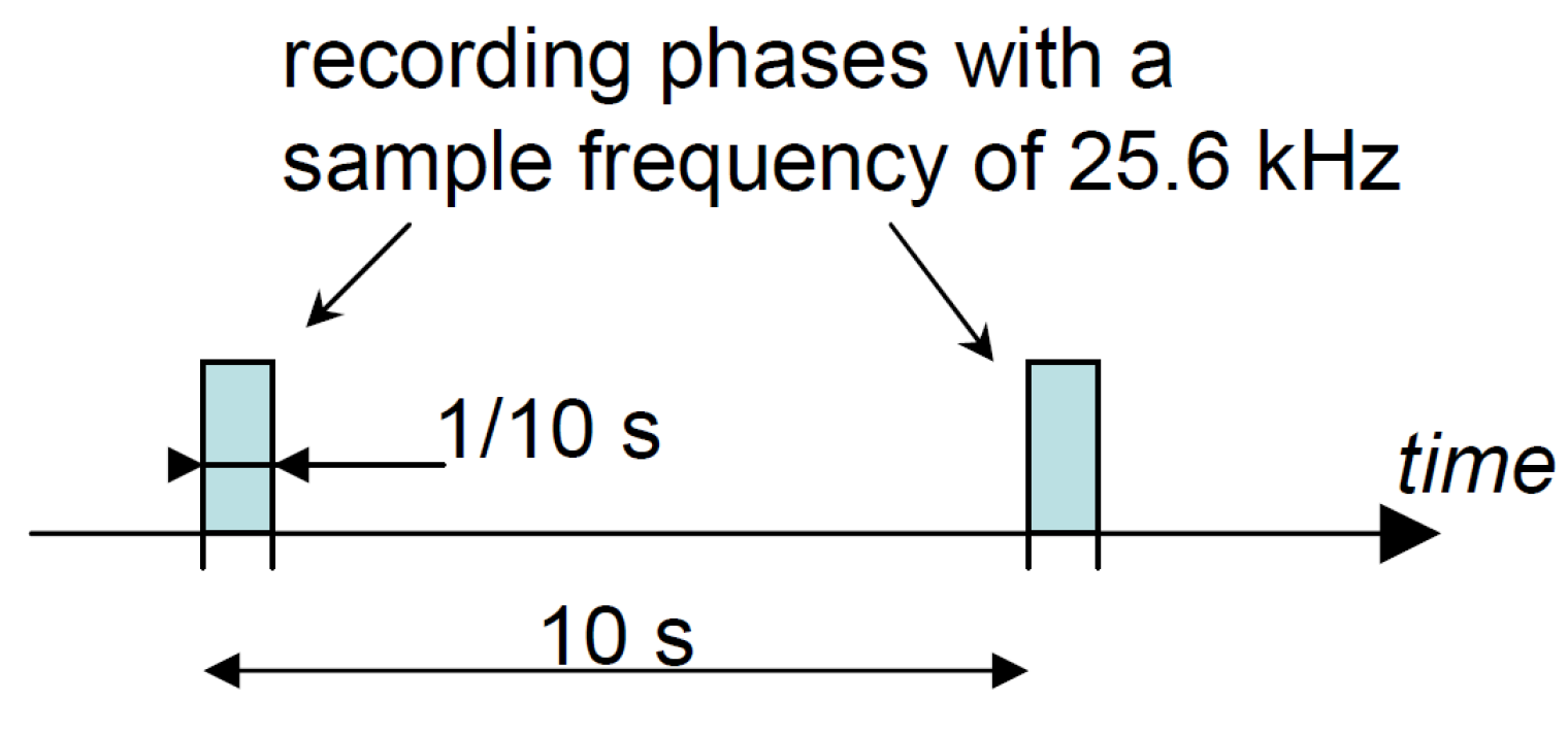
3.1. Testbed Preparation

As shown in Figure 4, the PRONOSTIA platform consist of a rotating part, a loading part, and a measurements part. The rotating part has an asynchronous motor with a speed reducer and two shafts. The power of the motor is 250 W, and the speed can reach 2830 rpm. After the transmission, the speed of the secondary shaft will work under 2000 rpm. The loading part is the key part of the whole system which is used to accelerate damage to the bearing. The radial force, acting on the bearing, could reach values up to 5000 N, which will significantly reduce this bearing’s life duration. The measurements part is responsible for collecting original data. There are two kinds of sensors in the system including vibration and temperature. The vibration sensors are located on the vertical axis and horizontal axis, respectively. The temperature sensor (PT100) is attached to the outer ring of the bearing. The vibration signal is sampled at 25.6 kHz, while the temperature is sampled at 10 Hz.
Figure 5 shows the vibration signal gathered during the overall run-to-failure experiment. The testbed was shut down when the amplitude of the vibration reached 20 g, which is the general ending criterion for all the bearing experiments. It is worth noting that the vibration signal is not continuously sampled during the experiment period. As shown in Figure 6, a vibration sample is collected after each specific time interval. The length of the sample is 2560 points, and the time interval is 10 s in each experiment.

3.2. Test Setting Details

In this work, we verified every part in the proposed predictive maintenance framework using the degradation vibration signal of rolling bearings. We selected the signal of B e a r i n g 1 _ 3 as the example to test the condition monitoring module. Two cases from different conditions including B e a r i n g 1 _ 3 and B e a r i n g 2 _ 6 were used to analyze the prognostic module. For the dynamic maintenance scheduling module, we assumed four bearings from the same condition including B e a r i n g 1 _ 1 , B e a r i n g 1 _ 3 , B e a r i n g 1 _ 5 , and B e a r i n g 1 _ 7 were working simultaneously. Meanwhile, B e a r i n g 1 _ 1 , B e a r i n g 1 _ 3 , B e a r i n g 1 _ 5 , and B e a r i n g 1 _ 7 were collected under the condition of the motor’s rotation speed was 1800 r/min and the load was 4000 N, and B e a r i n g 2 _ 6 were collected under the condition of the motor speed of 1650 r/min and the load of 4200 N. All the experiments had been tested on the computer with GPU of Nvidia GeForce GTX 2060 6 GB and CPU of Intel Core i7-10750H of 2.60 GHz.

3.3. Results and Analysis

3.3.1. Condition Monitoring Analysis

As the first step of our proposed method, the original vibration signal needed to be translated to more reasonable features based on the feature extraction method in Table 1. The extracted features are shown in Figure 7. F1–F6 are the RS features, and F7–F14 are the time-frequency domain features. It is obvious that most of the features are monotonous as time goes on, which means they either decrease or increase.
As explained in the condition monitoring section, it is really difficult to identify the performance of the equipment based on so many features shown in Figure 7. Therefore, we calculated the health index which is considered as reliable, combined with the extracted features. One example is shown in Figure 8, which is the reliability of the whole degradation process. The expert could easily make comprehensive decisions based on such an index.

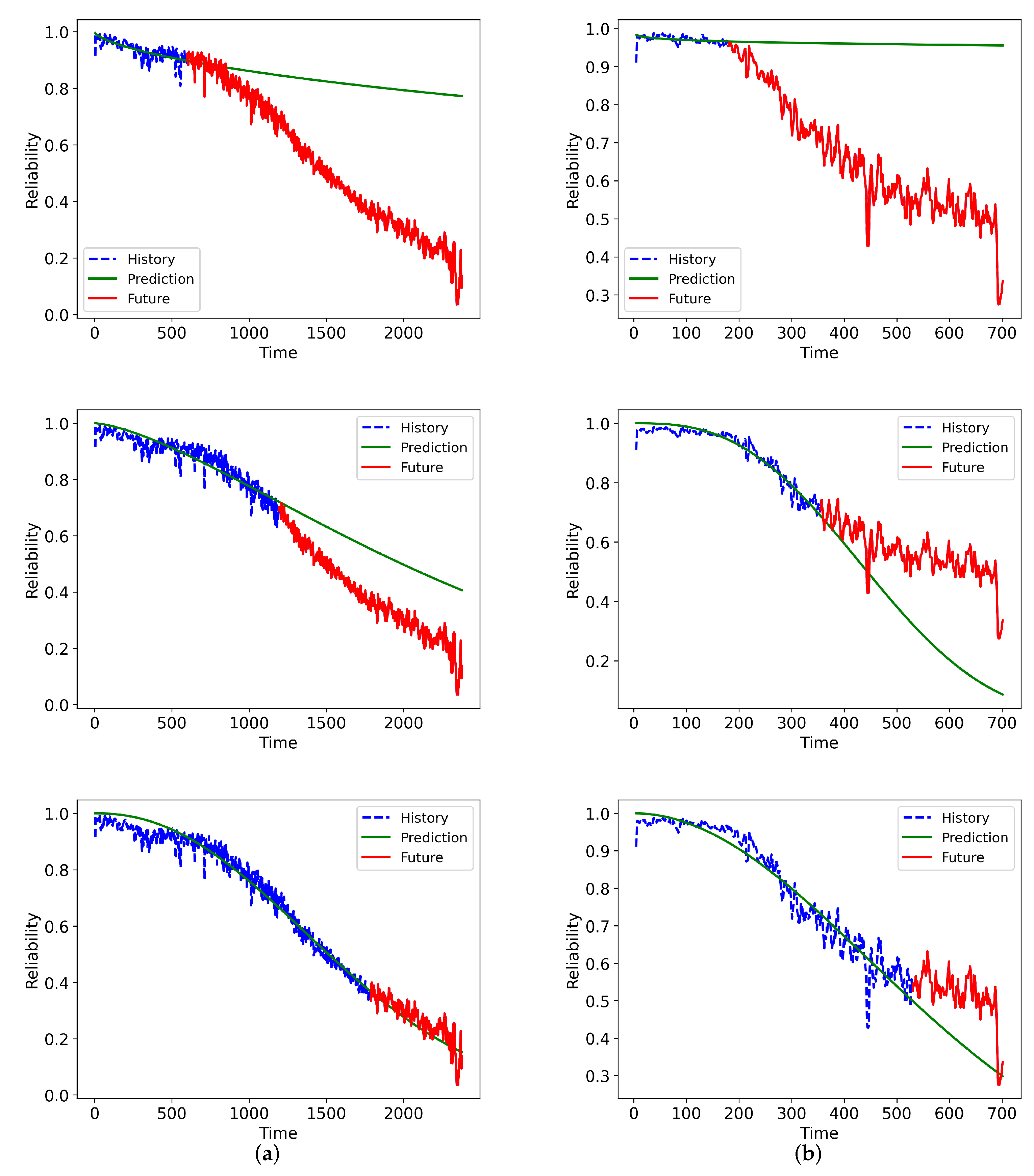
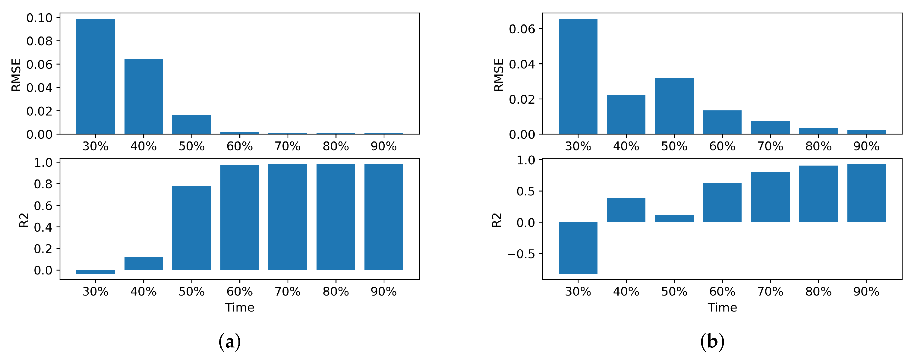
3.3.2. Prognositc Approach Analysis

Following the proposed framework, the analysis of the prognostic approach should be conducted once the degradation performance has been evaluated. As shown in Figure 9, the green line represents the learned reliability function, the blue line is the historical states, and the red line is the actual future state. It is obvious that the green line is close to the red line with the increase of the historical data ( 25 % , 50 % , and 75 % ). This means that the accuracy of the reliability increases as time progresses
For quantitative comparison of prognostic outcomes, two metrics including root mean square error (RMSE) and R2 are selected, which are defined as follows:
RMSE = 1 N i = 1 N ( r ^ i r i ) 2
R 2 = 1 i = 1 N ( r ^ i r i ) 2 i = 1 N ( r ^ i r ¯ ) 2
As shown in Figure 10, the RMSE is very large and the R2 is close to zero when the machine starts working after a while. In this period, the machine is operating under normal conditions, and the reliability should be close to 1. As degradation continues, the RMSE will decrease to zero, and the R2 will increase to 1. The results show that the reliability function will be highly accurate after accumulating a certain period of historical data. Based on the analysis of the results, it is obvious that the reliability function is dynamically changing where model parameters will be quickly updated once new data becomes available.
When the reliability function has been learned, the RUL could be predicted according to Equation (8). The prediction error E r t at each time step t is designed as:
E r t = A c t R U L t P r e d R U L t A c t R U L t
where A c t R U L t and P r e d R U L t are actual and predicted RUL value, respectively. As shown in Table 2, the RUL prediction values at different time steps are calculated. It is obvious that the errors ranging from 50 % to 80 % are closer to zero which means the RUL prediction results have a higher level of credibility.
To further analyze the proposed hybrid-based RUL module, we compared it with the two effective methods [36,38] experiment on the PRONOSTIA platform. As shown in Table 3, the results indicate that the proposed method performs better than other methods for B e a r i n g 1 _ 3 , while the performance under B e a r i n g 2 _ 6 is not as good as other methods.

3.3.3. Dynamic Maintenance Scheduling

The maintenance schedule is the outcome of the proposed predictive maintenance framework. Each bearing has its own reliability function, the manager could decide the maintenance time period based on the separate reliability functions. We assume that there are four bearings on a machine, then we could obtain all overall reliability as shown in Figure 11. Considering the suitable cost of remanufacturing, the threshold period of reliability is set to [ 0.25 , 0.4 ] . Then the separate maintenance period can be calculated as shown in Table 4. Based on the separate maintenance period, we could obtain the optimized period which could reduce the planned downtime frequency from four times to three times. Compared with the optimized results, the second strategy is better because the B e a r i n g 1 _ 1 could work more time.

4. Discussion and Conclusions

In the framework of the circular economy, industrial equipment is an important element in the manufacturing chain. The challenge facing managers in manufacturing sectors is to keep such equipment well-functioning because failure can result in a significant impact on productivity. Therefore, a reliable and dynamic predictive maintenance program is required to allow managers to make the right decision regarding remanufacturing of the equipment at the right time.
In this context, this paper proposed and presented a predictive maintenance framework for remanufacturing and explored the relationship between the PdM and remanufacturing. The dynamic maintenance scheduling has been proposed based on specific hybrid-based remaining useful lifetime prediction. The hybrid-based RUL prediction algorithm reaches the same level as other advanced prediction methods through the comparison and analysis of the rolling bearing degradation experiment. With the support of the presented prognostic approach, the dynamic maintenance framework enables fast real-time determination of the suitable time period for the equipment/components to be maintained or remanufactured so that machines are kept well-functioning and highly available in the production line.
The proposed framework will be implemented within RECLAIM (remanufacturing and refurbishment large industrial equipment) European-funded project [49]. RECLAIM seeks to establish solutions for the sake of helping European industry improve productivity and performance by addressing failure problem of aging equipment. The project aims to provide the foundation and tools that enable manufacturers to monitor the health conditions of machines and implement the appropriate remanufacturing strategy.
Future extensions that may be beneficial to the proposed framework include the following:
  • For the condition monitoring part, the more advanced algorithms can be investigated to improve the generalization of performance assessment and obtain more accurate reliability under different working conditions.
  • Based on the detailed analysis, the current algorithm used in the prognostic module could not work well when the machine working at the initial operation period has limited data. Therefore, prior knowledge of experts can be introduced to support the data limitation stage in future work.

Author Contributions

Conceptualization, M.Z. and Y.X.; methodology, M.Z. and N.A.; formal analysis, M.Z. and N.A.; investigation, M.Z.; writing—original draft preparation, M.Z. and Z.W.; writing—review and editing, N.A., Y.X. and A.M.; supervision, Y.X.; project administration, M.P.; funding acquisition, Y.X., M.P. and D.T. All authors have read and agreed to the published version of the manuscript.

Funding

This research was funded by RECLAIM project “Remanufacturing and Refurbishment Large Industrial Equipment” and received funding from the European Commission Horizon 2020 research and innovation programme under grant agreement No 869884.

Data Availability Statement

Data available in a publicly accessible repository that does not issue DOIs Publicly available datasets were analyzed in this study. This data can be found here: https://ti.arc.nasa.gov/tech/dash/groups/pcoe/prognostic-data-repository/ (accessed on 17 March 2022).

Conflicts of Interest

The authors declare no conflict of interest.

References

  1. U.S. Global Change Research Program. Global Climate Change Impacts in the United States; Technical Report; Cambridge University Press: Cambridge, UK, 2015. [Google Scholar]
  2. Dolge, K.; Blumberga, D. Key Factors Influencing the Achievement of Climate Neutrality Targets in the Manufacturing Industry: LMDI Decomposition Analysis. Energies 2021, 14, 8006. [Google Scholar] [CrossRef]
  3. Lin, Y.; Yang, H.; Ma, L.; Li, Z.; Ni, W. Low-Carbon Development for the Iron and Steel Industry in China and the World: Status Quo, Future Vision, and Key Actions. Sustainability 2021, 13, 12548. [Google Scholar] [CrossRef]
  4. Hu, X.; Yang, Z.; Sun, J.; Zhang, Y. Carbon tax or cap-and-trade: Which is more viable for Chinese remanufacturing industry? J. Clean. Prod. 2020, 243, 118606. [Google Scholar] [CrossRef] [Green Version]
  5. European Environment Agency. Circular Economy in Europe- Developing the Knowledge Base; Technical Report; Publications Office of the European Union: Luxembourg, 2015.
  6. Esposito, M.; Tse, T.; Soufani, K. Introducing a circular economy: New thinking with new managerial and policy implications. Calif. Manag. Rev. 2018, 60, 5–19. [Google Scholar] [CrossRef]
  7. D’Adamo, I. Adopting a circular economy: Current practices and future perspectives. Soc. Sci. 2019, 8, 328. [Google Scholar] [CrossRef] [Green Version]
  8. Zacharaki, A.; Vafeiadis, T.; Kolokas, N.; Vaxevani, A.; Xu, Y.; Peschl, M.; Ioannidis, D.; Tzovaras, D. RECLAIM: Toward a new era of refurbishment and remanufacturing of industrial equipment. Front. Artif. Intell. 2021, 3, 101. [Google Scholar] [CrossRef]
  9. Nußholz, J.L. Circular business models: Defining a concept and framing an emerging research field. Sustainability 2017, 9, 1810. [Google Scholar] [CrossRef] [Green Version]
  10. Charnley, F.; Tiwari, D.; Hutabarat, W.; Moreno, M.; Okorie, O.; Tiwari, A. Simulation to enable a data-driven circular economy. Sustainability 2019, 11, 3379. [Google Scholar] [CrossRef] [Green Version]
  11. Lee, C.M.; Woo, W.S.; Roh, Y.H. Remanufacturing: Trends and issues. Int. J. Precis. Eng.-Manuf.-Green Technol. 2017, 4, 113–125. [Google Scholar] [CrossRef]
  12. Siddiqi, M.U.; Ijomah, W.L.; Dobie, G.I.; Hafeez, M.; Pierce, S.G.; Ion, W.; Mineo, C.; MacLeod, C.N. Low cost three-dimensional virtual model construction for remanufacturing industry. J. Remanuf. 2019, 9, 129–139. [Google Scholar] [CrossRef] [Green Version]
  13. Diallo, C.; Venkatadri, U.; Khatab, A.; Bhakthavatchalam, S. State of the art review of quality, reliability and maintenance issues in closed-loop supply chains with remanufacturing. Int. J. Prod. Res. 2017, 55, 1277–1296. [Google Scholar] [CrossRef]
  14. Chen, L.; Wang, X.; Zhang, H.; Zhang, X.; Dan, B. Timing decision-making method of engine blades for predecisional remanufacturing based on reliability analysis. Front. Mech. Eng. 2019, 14, 412–421. [Google Scholar] [CrossRef]
  15. Lund, R.T.; Hauser, W.M. Remanufacturing-an American perspective. In Proceedings of the 5th International Conference on Responsive Manufacturing–Green Manufacturing (ICRM 2010), Ningbo, China, 11–13 January 2010. [Google Scholar]
  16. Du, Y.; Cao, H.; Liu, F.; Li, C.; Chen, X. An integrated method for evaluating the remanufacturability of used machine tool. J. Clean. Prod. 2012, 20, 82–91. [Google Scholar] [CrossRef]
  17. Selcuk, S. Predictive maintenance, its implementation and latest trends. Proc. Inst. Mech. Eng. Part J. Eng. Manuf. 2017, 231, 1670–1679. [Google Scholar] [CrossRef]
  18. Ortegon, K.; Nies, L.F.; Sutherland, J.W. The impact of maintenance and technology change on remanufacturing as a recovery alternative for used wind turbines. Procedia CIRP 2014, 15, 182–188. [Google Scholar] [CrossRef] [Green Version]
  19. Zonta, T.; da Costa, C.A.; da Rosa Righi, R.; de Lima, M.J.; da Trindade, E.S.; Li, G.P. Predictive maintenance in the Industry 4.0: A systematic literature review. Comput. Ind. Eng. 2020, 150, 106889. [Google Scholar] [CrossRef]
  20. Caggiano, A.; Segreto, T.; Teti, R. Cloud manufacturing framework for smart monitoring of machining. Procedia Cirp 2016, 55, 248–253. [Google Scholar] [CrossRef]
  21. Yan, R.; Gao, R.X.; Chen, X. Wavelets for fault diagnosis of rotary machines: A review with applications. Signal Process 2014, 96, 1–15. [Google Scholar] [CrossRef]
  22. Lei, Y.; Lin, J.; He, Z.; Zuo, M.J. A review on empirical mode decomposition in fault diagnosis of rotating machinery. Mech. Syst. Signal Process. 2013, 35, 108–126. [Google Scholar] [CrossRef]
  23. Zhang, M.; Jiang, Z.; Feng, K. Research on variational mode decomposition in rolling bearings fault diagnosis of the multistage centrifugal pump. Mech. Syst. Signal Process. 2017, 93, 460–493. [Google Scholar] [CrossRef] [Green Version]
  24. Zhao, R.; Yan, R.; Chen, Z.; Mao, K.; Wang, P.; Gao, R.X. Deep learning and its applications to machine health monitoring. Mech. Syst. Signal Process. 2019, 115, 213–237. [Google Scholar] [CrossRef]
  25. Zhang, M.; Wang, D.; Lu, W.; Yang, J.; Li, Z.; Liang, B. A deep transfer model with wasserstein distance guided multi-adversarial networks for bearing fault diagnosis under different working conditions. IEEE Access 2019, 7, 65303–65318. [Google Scholar] [CrossRef]
  26. Wang, D.; Zhang, M.; Xu, Y.; Lu, W.; Yang, J.; Zhang, T. Metric-based meta-learning model for few-shot fault diagnosis under multiple limited data conditions. Mech. Syst. Signal Process. 2021, 155, 107510. [Google Scholar] [CrossRef]
  27. Shin, J.H.; Cho, Y.H. Machine-Learning-Based Coefficient of Performance Prediction Model for Heat Pump Systems. Appl. Sci. 2022, 12, 362. [Google Scholar] [CrossRef]
  28. Si, X.S.; Wang, W.; Hu, C.H.; Zhou, D.H. Remaining useful life estimation–a review on the statistical data driven approaches. Eur. J. Oper. Res. 2011, 213, 1–14. [Google Scholar] [CrossRef]
  29. Lei, Y.; Li, N.; Guo, L.; Li, N.; Yan, T.; Lin, J. Machinery health prognostics: A systematic review from data acquisition to RUL prediction. Mech. Syst. Signal Process. 2018, 104, 799–834. [Google Scholar] [CrossRef]
  30. Zhang, Z.; Si, X.; Hu, C.; Lei, Y. Degradation data analysis and remaining useful life estimation: A review on Wiener-process-based methods. Eur. J. Oper. Res. 2018, 271, 775–796. [Google Scholar] [CrossRef]
  31. Wang, C.; Jiang, W.; Yang, X.; Zhang, S. RUL Prediction of Rolling Bearings Based on a DCAE and CNN. Appl. Sci. 2021, 11, 11516. [Google Scholar] [CrossRef]
  32. Wang, B.; Lei, Y.; Li, N.; Li, N. A hybrid prognostics approach for estimating remaining useful life of rolling element bearings. IEEE Trans. Reliab. 2018, 69, 401–412. [Google Scholar] [CrossRef]
  33. Lei, Y.; Li, N.; Gontarz, S.; Lin, J.; Radkowski, S.; Dybala, J. A model-based method for remaining useful life prediction of machinery. IEEE Trans. Reliab. 2016, 65, 1314–1326. [Google Scholar] [CrossRef]
  34. Li, N.; Lei, Y.; Lin, J.; Ding, S.X. An improved exponential model for predicting remaining useful life of rolling element bearings. IEEE Trans. Ind. Electron. 2015, 62, 7762–7773. [Google Scholar] [CrossRef]
  35. Qian, Y.; Yan, R. Remaining useful life prediction of rolling bearings using an enhanced particle filter. IEEE Trans. Instrum. Meas. 2015, 64, 2696–2707. [Google Scholar] [CrossRef]
  36. Hong, S.; Zhou, Z.; Zio, E.; Hong, K. Condition assessment for the performance degradation of bearing based on a combinatorial feature extraction method. Digit. Signal Process. 2014, 27, 159–166. [Google Scholar] [CrossRef]
  37. Ren, L.; Sun, Y.; Wang, H.; Zhang, L. Prediction of bearing remaining useful life with deep convolution neural network. IEEE Access 2018, 6, 13041–13049. [Google Scholar] [CrossRef]
  38. Guo, L.; Li, N.; Jia, F.; Lei, Y.; Lin, J. A recurrent neural network based health indicator for remaining useful life prediction of bearings. Neurocomputing 2017, 240, 98–109. [Google Scholar] [CrossRef]
  39. Wang, Z.; Xu, Y.; Ma, X.; Thomson, G. Towards smart remanufacturing and maintenance of machinery-review of automated inspection, condition monitoring and production optimisation. In Proceedings of the 2020 25th IEEE International Conference on Emerging Technologies and Factory Automation (ETFA), Vienna, Austria, 8–11 September 2020; Volume 1, pp. 1731–1738. [Google Scholar]
  40. Schmidt, B.; Wang, L. Cloud-enhanced predictive maintenance. Int. J. Adv. Manuf. Technol. 2018, 99, 5–13. [Google Scholar] [CrossRef]
  41. Calabrese, F.; Regattieri, A.; Botti, L.; Mora, C.; Galizia, F.G. Unsupervised fault detection and prediction of remaining useful life for online prognostic health management of mechanical systems. Appl. Sci. 2020, 10, 4120. [Google Scholar] [CrossRef]
  42. Mao, W.; He, J.; Zuo, M.J. Predicting remaining useful life of rolling bearings based on deep feature representation and transfer learning. IEEE Trans. Instrum. Meas. 2019, 69, 1594–1608. [Google Scholar] [CrossRef]
  43. Jin, X.; Ma, E.W.; Chow, T.W.; Pecht, M. An investigation into fan reliability. In Proceedings of the IEEE 2012 Prognostics and System Health Management Conference (PHM-2012 Beijing), Beijing, China, 23–25 May 2012; pp. 1–7. [Google Scholar]
  44. Jia, P.; Liu, H.; Zhu, C.; Wu, W.; Lu, G. Contact fatigue life prediction of a bevel gear under spectrum loading. Front. Mech. Eng. 2020, 15, 123–132. [Google Scholar] [CrossRef] [Green Version]
  45. Li, Y.; Zhu, C.; Chen, X.; Tan, J. Fatigue Reliability Analysis of Wind Turbine Drivetrain Considering Strength Degradation and Load Sharing Using Survival Signature and FTA. Energies 2020, 13, 2108. [Google Scholar] [CrossRef]
  46. Nocedal, J.; Wright, S.J. Numerical Optimization; Springer: Berlin/Heidelberg, Germany, 1999. [Google Scholar]
  47. Durazo-Cardenas, I.; Starr, A.; Turner, C.J.; Tiwari, A.; Kirkwood, L.; Bevilacqua, M.; Tsourdos, A.; Shehab, E.; Baguley, P.; Xu, Y.; et al. An autonomous system for maintenance scheduling data-rich complex infrastructure: Fusing the railways’ condition, planning and cost. Transp. Res. Part Emerg. Technol. 2018, 89, 234–253. [Google Scholar] [CrossRef]
  48. Nectoux, P.; Gouriveau, R.; Medjaher, K.; Ramasso, E.; Chebel-Morello, B.; Zerhouni, N.; Varnier, C. PRONOSTIA: An experimental platform for bearings accelerated degradation tests. In Proceedings of the IEEE International Conference on Prognostics and Health Management, PHM’12, Denver, CO, USA, 18–21 June 2012; pp. 1–8. [Google Scholar]
  49. RECLAIM. RE-manufaCturing and Refurbishment LArge Industrial Equipment. Available online: https://www.reclaim-project.eu/ (accessed on 18 March 2022).
Figure 1. The relationship between remaufacturability and predictive maintenance.
Applsci 12 03218 g001
Figure 2. The overview of proposed predictive maintenance architecture.
Applsci 12 03218 g002
Figure 3. The workflow of dynamic maintenance scheduling.
Applsci 12 03218 g003
Figure 4. The testbed of bearing degradation experiment.
Applsci 12 03218 g004
Figure 5. Vibration signal from normal to the degraded condition in an experiment.
Applsci 12 03218 g005
Figure 6. Sampling interval description of vibration signals.
Applsci 12 03218 g006
Figure 7. Extracted features of B e a r i n g 1 _ 3 with whole degradation process.
Applsci 12 03218 g007
Figure 8. Degradation performance assessment of B e a r i n g 1 _ 3 .
Applsci 12 03218 g008
Figure 9. Learned reliability function from the historical data of 25 % , 50 % , and 75 % during the whole degradation period: (a) B e a r i n g 1 _ 3 ; (b) B e a r i n g 2 _ 6 .
Applsci 12 03218 g009
Figure 10. The quantitative comparison results of learned reliability function under different historical data percentages: (a) B e a r i n g 1 _ 3 ; (b) B e a r i n g 2 _ 6 .
Applsci 12 03218 g010
Figure 11. Gantt chart of maintenance scheduling results.
Applsci 12 03218 g011
Table 1. Detailed features description.
RS FeaturesEnergy Ratio Features
Time-DomainFrequency-DomainTime-Frequency-Domain
F1RS of 11 classicalF2RS of [0, 12.8 kHz]F7Energy ratio of (3, 0)
time-domainF3RS of [0, 3.2 kHz]F8Energy ratio of (3, 1)
featuresF4RS of [3.2 kHz, 6.4 kHz]F9Energy ratio of (3, 2)
F5RS of [6.4 kHz, 9.6 kHz]F10Energy ratio of (3, 3)
F6RS of [9.6 kHz, 12.8 kHz]F11Energy ratio of (3, 4)
F12Energy ratio of (3, 5)
F13Energy ratio of (3, 6)
F14Energy ratio of (3, 7)
Table 2. RUL prediction results under different historical data percentages.
Bearing 1 _ 3 Bearing 2 _ 6
Time ProportionActual RUL (s)Predicted RUL (s)Er (%)Actual RUL (s)Predicted RUL (s)Er (%)
30 % 16,590483,400−2813.804870472,840−9609.24
40 % 14,210100,030−603.944170357014.38
50 % 11,84023,430−97.883470249028.24
60 % 94609960−5.28277027201.80
70 % 7090578018.4720702710−30.91
80 % 4710319032.2713703140−129.19
90 % 2340121048.296703510−423.88
Table 3. RUL prediction results compared with other methods.
Current Time (s)Actual RUL (s)Predicted RUL (s)Er (%)Er of [36] (%)Er of [38] (%)
B e a r i n g 1 _ 3 18,0105730410028.44−31.7643.28
B e a r i n g 2 _ 6 571012903170−145.73−51.94−13.95
Table 4. Detailed results of Maintenance scheduling.
Maintenance PeriodOptimized Maintenance Period
Orignal12
B e a r i n g 1 _ 1 [1708, 2563][1719, 2071][2305, 2563]
B e a r i n g 1 _ 3 [1719, 2071][1719, 2071][1719, 2071]
B e a r i n g 1 _ 5 [2305, 3429][2305, 3429][2305, 2563]
B e a r i n g 1 _ 7 [1142, 1334][1142, 1334][1142, 1334]
Publisher’s Note: MDPI stays neutral with regard to jurisdictional claims in published maps and institutional affiliations.

