Identification and Reconstruction of Impact Load for Lightweight Design of Production Equipment

Abstract

This paper proposes a method for determining externally applied impact loads on complex structures using strain analysis. An impact load transducer was developed to determine impact loads. Using this transducer (which incorporates strain gauges), the relationship between the measured strains and applied impact load was studied, and a model for conversion from strain analysis to impact load was developed. The reconstructed impact curve that characterizes the impact peak force, impact duration, and load in the steady state after impact was employed as an input load curve in finite element analysis. The reconstructed impact load was validated by comparing the structural strain measured on the specimen in the experiments and the strain calculated by the simulations. The results show that the maximum difference between experimentally and numerically determined structural peak strains is 3.2 με. Moreover, the method was validated by predicting the impact load of a descending vehicle chassis on the production equipment in an automotive production line. It demonstrated high efficiency and accuracy. The reconstructed load curve obtained using the developed method provides high efficiency in addition to high accuracy. Furthermore, it circumvents the complexities of modeling dynamic impact simulation, including complex impactor shape, interface, and friction conditions. Thus, the developed method provides scholars with an efficient approach for an extensive study of the responses of complex structures in various fields such as stress strain analysis, fatigue analysis, and topology optimization for lightweight design of production equipment.

1. Introduction

The external impact load on production equipment such as jigs and fixtures makes them vulnerable to various types of structural failure including structural deformation, fatigue failure, and joint loosening, which reduce their load-carrying capabilities. The use of lightweight materials [1,2] and optimization of structures in industries such as automotive and aerospace [3,4] have reduced the impact load on production equipment, thus reducing damage of contacting structures at impact. Under these circumstances, production equipment should also be optimized to reduce operational energy consumption while maintaining the manufacturing quality. To achieve this, the capability to predict an externally applied impact load is required for a sophisticated investigation of the structural behavior under impact during manufacturing.

During the past decades, research on impact events has been carried out by employing numerical simulations. Numerical simulations have been performed to investigate the behavior of equipment under impact without accurately identifying the impact during manufacturing. Zhao et al. [5] investigated the impact and post-impact behavior of H-shaped steel members by modeling a simplified impact hammer. Ince et al. [6] constructed an FE model of an ice drop test to determine the crashworthiness in the event of a ship colliding with an ice-ridge. Khan and Sonawane [7] presented FE simulations of impact loading on a construction safety helmet by a striker to improve the ventilation slot profile in helmet design. Kishi et al. [8] also established an FE simulation of falling-weight impact events to analyze the dynamic response of a reinforced concrete beam. However, these numerical studies require the modeling of a contact interface subjected to a dynamic impact, which is impractical [9]. In addition, the shapes of the impactors used in the studies mentioned above were either of simplified types or early elementary designs, which were dissimilar to the complex shapes of products. Yao et al. [10] observed that the structural behavior under impact depends strongly on the shape of the impactor. However, in industrial production lines, it is unfeasible to simplify the shape of objects that apply load, such as vehicle chassis, because of the complexity involved. Meanwhile, the development of a complete model of an impactor requires a substantial amount of time for modeling the detailed specifications and is computationally expensive. Moreover, it is noteworthy that several production equipment holding objects that apply load generally contains deviations in specification. This causes the production equipment in a real production line to be loaded unequally. Thus, a practical and accurate method for identifying complex impactor-induced structural responses is required.

Reconstruction of impact load based on measurable system behavior [11,12,13,14] (e.g., acceleration, strain, and displacement) also enables us to investigate the dynamic response of structures. Previous works aimed to reconstruct impact load by solving mathematical models that were developed from the elasticity theory or modal analysis [11,15,16]. Because mathematical models are generally derived from the linear behavior of systems, the mathematical analysis is restricted to linear structures such as a beams or plates. In addition, the proposed methods showed varying levels of accuracy with solution instability and ill-posedness. To overcome this problem, researchers introduced Tikhonov regularization methods [17] and singular value decomposition (SVD) methods [18]. However, these methods are computationally inefficient while addressing large-scale inverse problems. Other regularization methods including the function expansion method [12,19] and Levenberg–Marquardt regularization method [20] were also introduced. Although the basis function expansion method resolves the problem of large-scale inverse problems, the critical problem of selecting the type and number of basis functions remains. The technique using the Levenberg–Marquardt method also involves the intricate problem of selecting the correct regularization parameter. A probabilistic method using Kalman filtering [21] was also proposed to stabilize the solution. Although the instability problem was mostly resolved, the reconstructed force quality appeared to degrade with the increase in system noise. In addition to regularization and probabilistic methods, Simone et al. [22] proposed a method to use the experimentally measured response of a composite structure to calibrate the transfer function between the acquired response and the impact load. However, the proposed method requires the calibration of the transfer function from an exceptionally large amount of training data for a single structure. Recently, neural networks were employed to predict the impact loads acting on a simple nonlinear system [23,24,25]. Although studies using neural networks succeeded in predicting the impact force applied on simple nonlinear structures such as composite plates, the results showed variation in responses according to the material properties and geometry. Large amounts of training data must be accumulated for effective practical applications of neural networks. Thus, the reconstruction of the impact load applied to complex production equipment (which is generally assembled with various parts made of different types of material) continues to be a challenging task.

This paper presents a method for identifying an unknown impact load through strain analysis with a newly designed transducer. We designed the transducer with strain gauges and reconstructed the impact load by developing a conversion model based on strain analysis. The reconstructed impact load was employed as an input load curve in the finite element analysis. Furthermore, it was validated by comparing the strain measured on an experimental specimen and that calculated by the simulations. Finally, the developed method was validated by reconstructing the impact load by a vehicle chassis on the engineering jig structure in the vehicle production line of Hyundai Motors, for the design of lightweight production equipment.

2. Methodology for Identifying Unknown Impact Load

2.1. Identification of Impact Load

The method used to identify the external impact load acting on production equipment (jig structure) is outlined in Figure 1. First, the external impact load is obtained by measuring a time-domain strain signal acquired using a newly designed transducer incorporated with strain gauges, i.e., an impact load transducer. Next, the strain signal is converted to load data. These are subsequently utilized to reconstruct the external impact load from the input data, in the FE analysis of the engineering structure.

2.2. Impact Load Reconstruction through Strain–Load Conversion

A direct measurement of the impact force is not feasible in the general condition of manufacturing processes. Considering this, a small transducer was manufactured to accurately determine an arbitrary unknown impact load from strain signals. To measure the compressive strain signals, the axis of the strain gauges is aligned in the direction of the applied load. KFG-02-120-C1-11 uniaxial strain gauges of 120 Ω from KYOWA are used in this study (Figure 1b). As shown in Figure 1b, the impact load transducer was calibrated under uniaxial compression conditions using a universal testing machine (UTM). The tests were performed at a testing rate of 10 mm/s. Five sets of loads were applied in the axial direction, and five points were recorded for each set. The specimen was loaded to 3 kN, and the force from the UTM and the output signals from the four strain gauges were recorded. A digital meter (System 7000 Strain Smart Data Acquisition System from Vishay Micro-Measurements) was used to record the resistance change of the strain gauge with a sampling rate of 2000 Hz. The average of the four strain gauge signals (με) was calibrated with the load data, as shown in Figure 1b. The developed converting model shows good agreement with the actual applied load (Figure 1c) and an R² value of 0.9945. Thus, the average of the strain values can be converted to a load as expressed in Equation (1):

$$\mathrm{Load}=6.82·\mathrm{Average} \mathrm{Strain}+20.51$$

(1)

3. Validation with Specimen Experiments

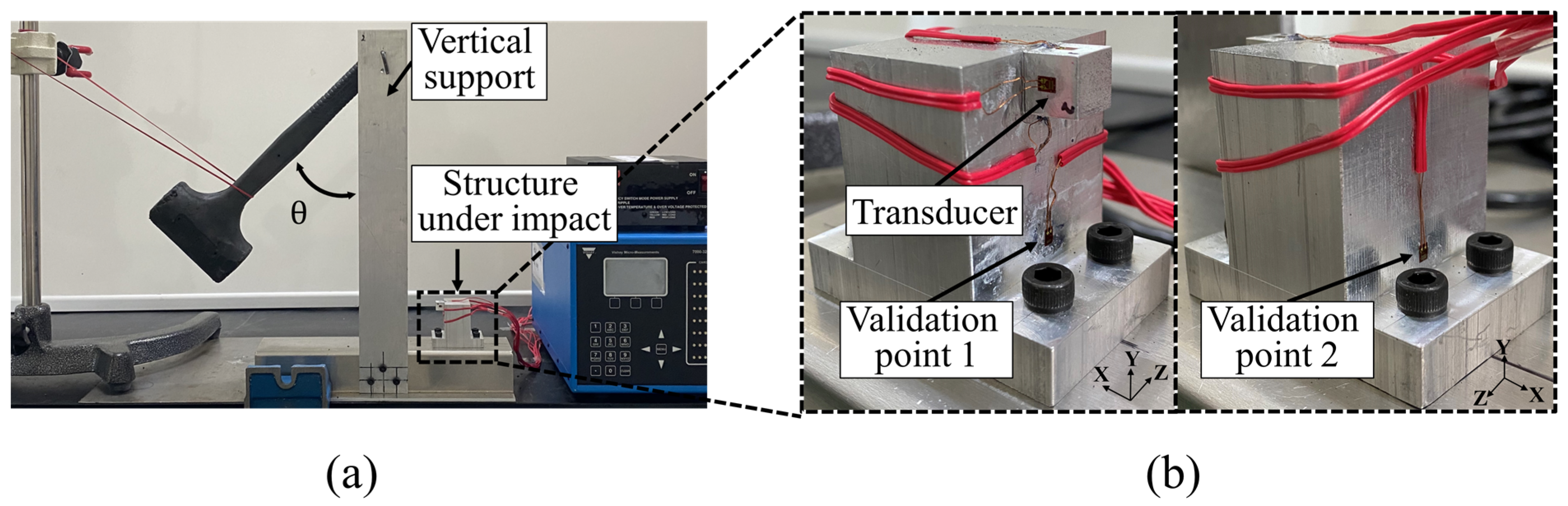
3.1. Experimental Set-Up

The impact-testing apparatus is designed to obtain strain signals of the transducer when it is subjected to external impact, as shown in Figure 2a. The impact load transducer is fixed at a static point of a structure where the impact is applied. It collects the impact-induced time-domain strain signal. Its impact energy is adjusted by the angle between the impactor arm and vertical supports. In this study, the impactor angle was set as 32°, 47°, and 65° for each experiment. Two strain gauges are attached to the front and back surfaces of the structure to directly measure the transient strain signals of the structure during external impact, as shown in Figure 2b.

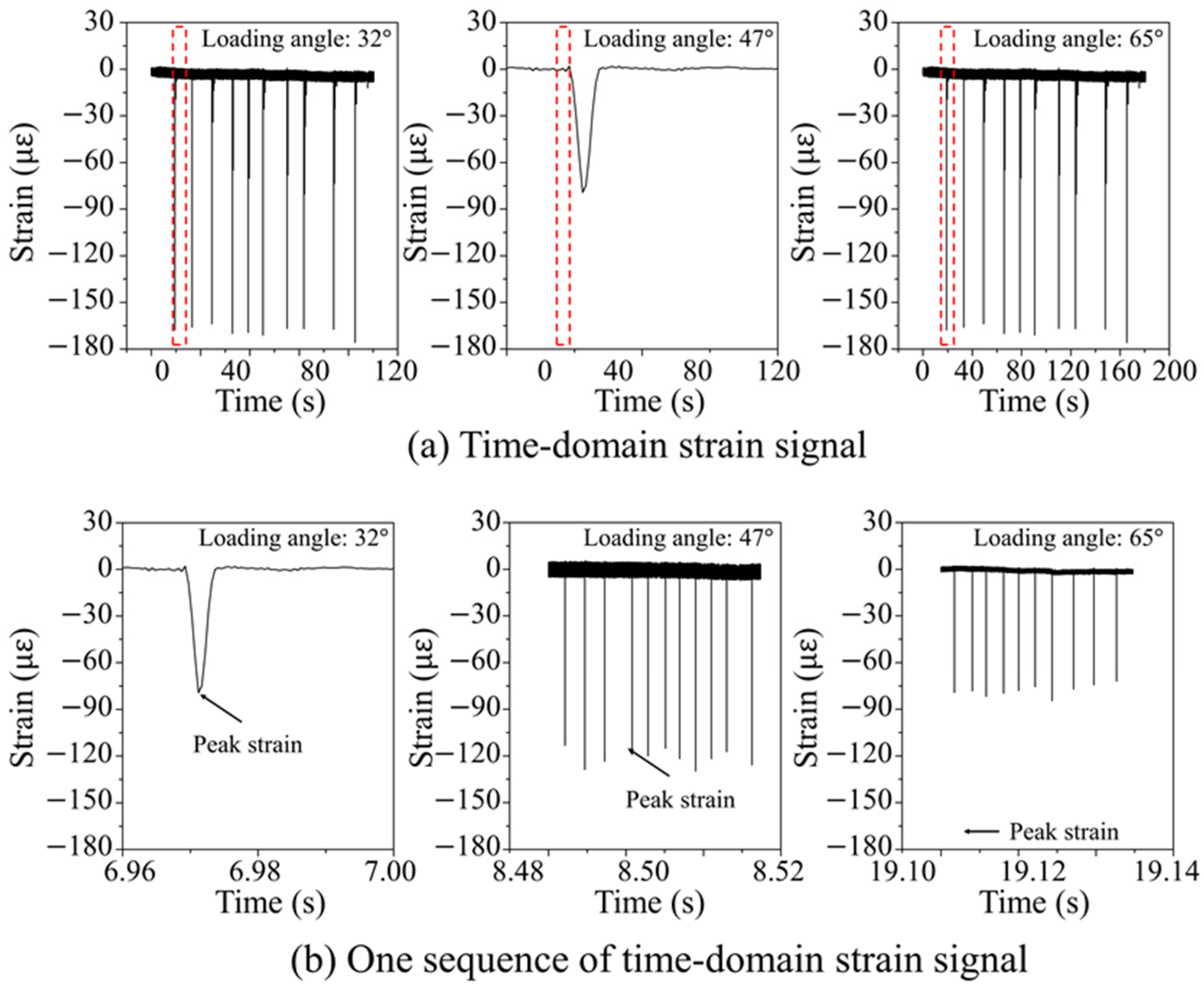
3.2. Experimental Results

The structure is subject to three impact loads. The time-domain strain signal is recorded by the transducer for 10 consecutive impacts, as shown in Figure 3a. An inspection of a sequence of the strain signal reveals that the peak strain of the impact increases with an increase in the impactor angle. The increase in impactor angle results in a higher impact energy, which, in turn, causes an increase in strain. The peak strains and impact durations for all the experiments are listed in

Table 1. Strain data measured with impact load transducer in impact experiments.

	Loading Angle: 32°		Loading Angle: 47°		Loading Angle: 65°
Set	Peak Strain $\left(\mathit{\mu }\right)$	Impact Duration (s)	Peak Strain $\left(\mathit{\mu }\right)$	Impact Duration (s)	Peak Strain $\left(\mathit{\mu }\right)$	Impact Duration (s)
1.	−79.25	0.0044	−113.25	0.0044	−167.75	0.0044
2.	−78.25	0.0044	−128.75	0.0048	−166.00	0.0044
3.	−81.75	0.0044	−123.50	0.0048	−163.75	0.0044
4.	−79.75	0.0044	−119.25	0.0049	−170.00	0.0044
5.	−78.00	0.0044	−120.00	0.0044	−169.25	0.0044
6.	−75.50	0.0044	−115.00	0.0049	−171.00	0.0049
7.	−84.50	0.0044	−129.75	0.0044	−166.75	0.0044
8.	−77.00	0.0044	−121.75	0.0040	−167.00	0.0044
9.	−74.25	0.0049	−116.00	0.0049	−167.25	0.0044
10.	−72.00	0.0044	−125.75	0.0044	−175.25	0.0044
Standard deviation	3.63	0.0002	5.68	0.0003	3.18	0.0002
Average	−79.25	0.0045	−121.30	0.0046	−168.40	0.0045

. The experiments with the impactor loading angles of 32°, 47°, and 65° show average peak strains of −79.25, −121.30, and 168.40 με, respectively, and standard deviations of 3.63, 5.68, and 3.18 με, respectively. All the strain responses returned to their original state after the peak strain. The impact duration is determined by the duration of the high strain rate region before and after the peak strain. The three experiments had nearly identical average impact durations.

3.3. Reconstruction of Impact Load

The impact-induced strain acquired from the impact load transducer can be utilized to determine the impact load for FE analysis. The important parameters that characterize an impact are the impact peak force, impact duration, and load in the steady state after impact. Although certain studies have converted dynamic loads into equivalent static loads, a static load cannot represent dynamic effects, particularly peak loads that result from dynamic impact. Investigations of the peak load magnitude and timing of a beam structure under impulse loads of triangular, sinusoidal, and trapezoidal shapes showed that simulations using the triangular load curves display the highest agreement with the results of the actual impact [26]. The results of our specimen experiments also illustrate that the time-domain strain signal measured by the transducer can be characterized by peak strain and impact duration. This demonstrates the validity of the adoption of a triangular load curve. In all the three experiments, the impact duration was divided uniformly by the peak strain point. Thus, we reconstructed the impact load by adopting a triangular shape, which is defined by the peak load magnitude and impact duration. The average strain value is converted to a load by using the developed model, as shown in Equation (1). The load curves for the three laboratory impact experiments with different loading angles are reconstructed based on the average strain data of 10 consecutive impacts (Figure 4).

3.4. Validation of Reconstructed Impact Load with Structural Strain

The accuracy of our method is examined by investigating whether the FE simulation model applied with the reconstructed impact load generates maximum strain responses similar to those of the actual dynamic impact experiments, as shown in Figure 2b. The measured strains induced by impact at two validation points of the structure are compared with the corresponding strains from the numerical simulations. The strain measured at Validation points 1 and 2 are the y-axis strain, as shown in Figure 2b and Figure 5. The y-axis strains of Validation points 1 and 2 are caused mainly by the bending force induced by the impact load. Figure 5a,b shows the contour representations of the distributions of strains in the y-axis and the elements used for calculating the strains at the validation points. As shown in Figure 5c, a positive strain is caused by the tensile stress at Validation point 1, whereas a negative strain is caused by the compressive stress at Validation point 2. The error bars in the experimental data describe the deviation in the strain data measured in 10 sets of impact experiments. The peak strains at the validation points measured in the experiments are listed in

Table 2. Peak strain data measured at validation points in the lab-scale impact experiments.

	Validation Point 1			Validation Point 2
	65°	47°	32°	65°	47°	32°
Set	$\mathbf{Peak} \mathbf{Strain} \left(\mathit{\mu }\right)$	$\mathbf{Peak} \mathbf{Strain} \left(\mathit{\mu }\right)$	$\mathbf{Peak} \mathbf{Strain} \left(\mathit{\mu }\right)$	$\mathbf{Peak} \mathbf{Strain} \left(\mathit{\mu }\right)$	$\mathbf{Peak} \mathbf{Strain} \left(\mathit{\mu }\right)$	$\mathbf{Peak} \mathbf{Strain} \left(\mathit{\mu }\right)$
1.	78.00	52.00	39.00	−81.00	−51.00	−41.00
2.	76.00	57.00	36.00	−84.00	−60.00	−39.00
3.	76.00	51.00	37.00	−83.00	−62.00	−39.00
4.	74.00	48.00	38.00	−79.00	−64.00	−41.00
5.	74.00	57.00	38.00	−86.00	−60.00	−42.00
6.	71.00	58.00	38.00	−81.00	−55.00	−39.00
7.	78.00	56.00	37.00	−80.00	−58.00	−43.00
8.	73.00	52.00	36.00	−81.00	−53.00	−41.00
9.	76.00	54.00	37.00	−77.00	−51.00	−42.00
10.	78.00	50.00	36.00	−75.00	−56.00	−39.00
Standard deviation	2.37	3.41	1.03	3.23	1.55	1.65
Average	75.40	53.50	37.20	−80.70	−57.00	−40.50

. The error bars in the numerical simulation are presented to illustrate the uncertainty in the position of the validation points in the numerical model. Six elements selected at each validation point are shown in Figure 5a,b. The average peak strain measured at the two validation points for the loading angle of 32° are 37.2 and −80.7 με, respectively, whereas the calculated values are 35.2 and −81.8 με, respectively. The average peak strain measured at the two validation points for the loading angle of 47° are 53.5 and −54.0 με, respectively, whereas the calculated values are 54.4 and −56.7 με, respectively. The average peak strain measured at the two validation points for the loading angle of 65° are 75.4 and −80.7 με, respectively, whereas the calculated values are 78.6 and −81.8 με, respectively. The maximum difference between experimentally measured and numerically calculated peak strain is 3.2 με This is observed at Validation point 1 with the loading angle of 65°, which corresponds to the highest impact. The remarkable agreement indicates that the system developed in this study can determine externally applied impact loads with sufficient accuracy.

4. Validation with Automotive Production Equipment: Jig Structure

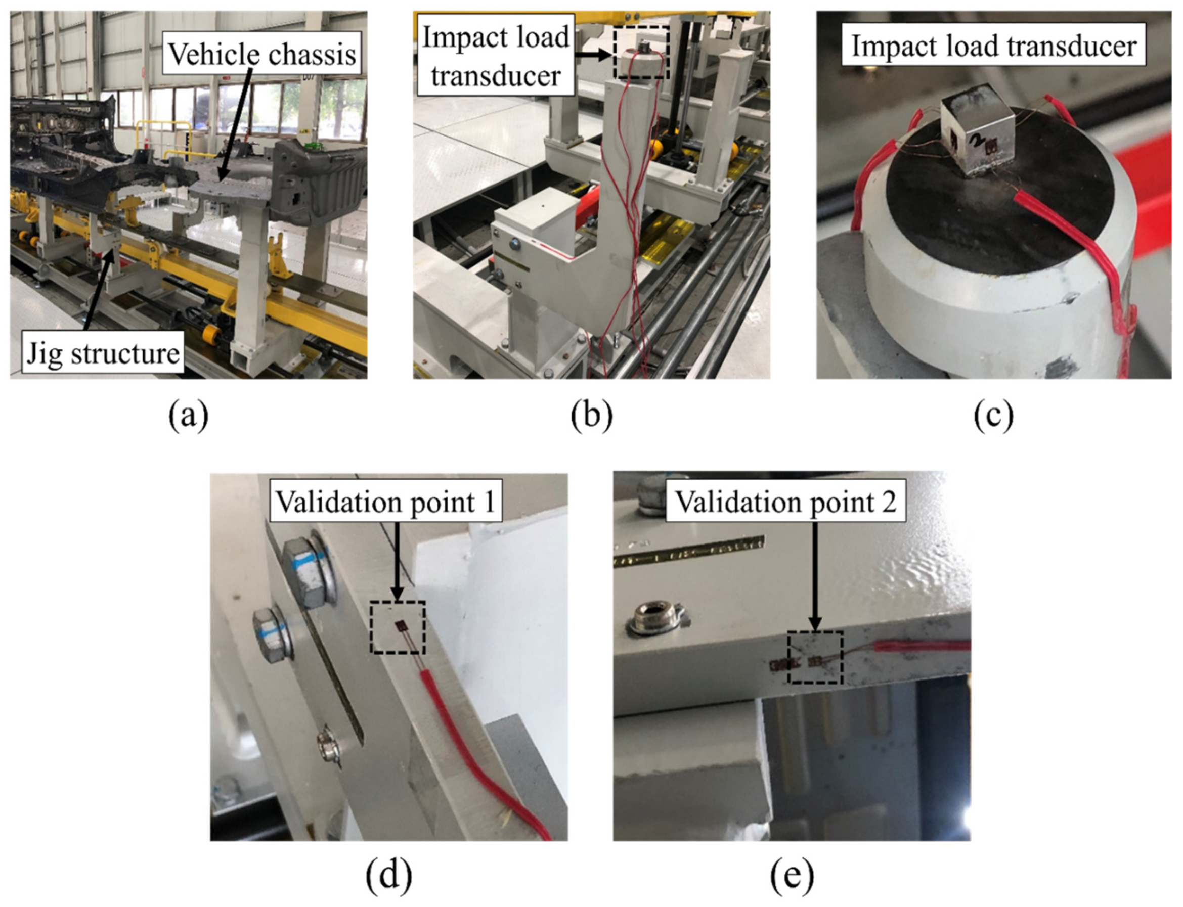
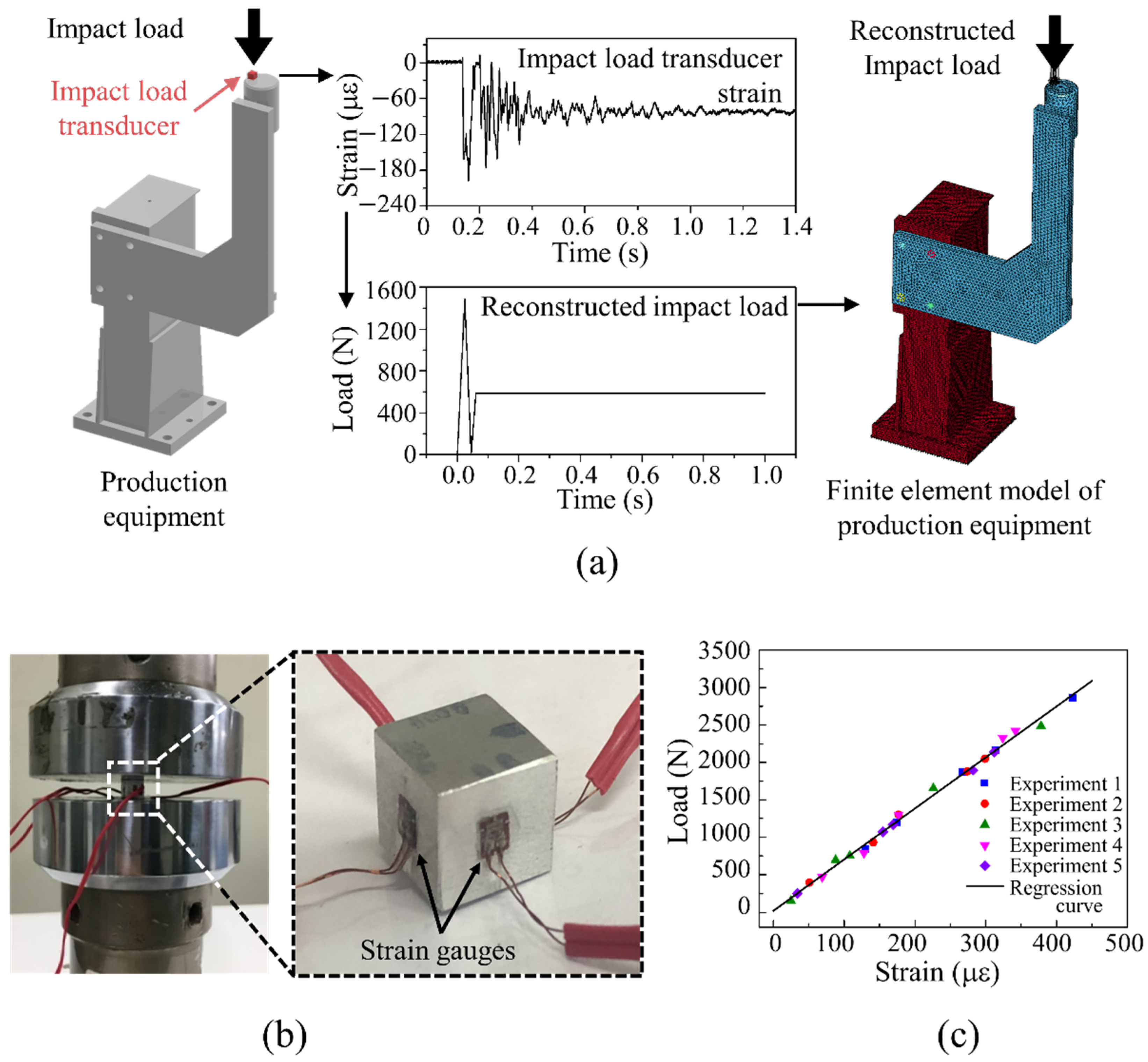
4.1. Experimental Set-Up

The method developed for identifying impact loads was validated at a practical scale. During the vehicle manufacturing process, production equipment such as the jig structure sustain the impact load of descending vehicle chassis. Impact experiments with vehicle chassis were conducted in the Hyundai Motors production line. The loading speeds of the vehicle chassis are controlled by varying the pressure of the hydraulic system. In this experiment, two loading velocities were examined: 246.8 and 287.4 mm/s. To obtain accurate strain data from the impact load transducer, 11 sets of impact experiments were performed for each loading velocity. The production line with jig structures and vehicle chassis is presented in Figure 6a, and an individual jig structure is shown in Figure 6b. To determine the impact load provided by a descending vehicle chassis, the impact load transducer was mounted at the point of contact between the jig structure and vehicle chassis, as shown in Figure 6c. Because the loading position has a circular cavity, the impact load transducer was mounted at a marginal distance from the center of the impact point to ensure complete contact between the impact load transducer and vehicle chassis. To validate the predicted impact load, strain gauges were attached to the jig structures to measure the strain generated in the jig structure by the impact of vehicle chassis. Three regions with high strain were selected as the validation points, as shown in Figure 6d,e. The structural strains measured at the validation points in the experiments were compared with the strains calculated by numerical simulation using the impact load predicted by the method developed for determining impact loads.

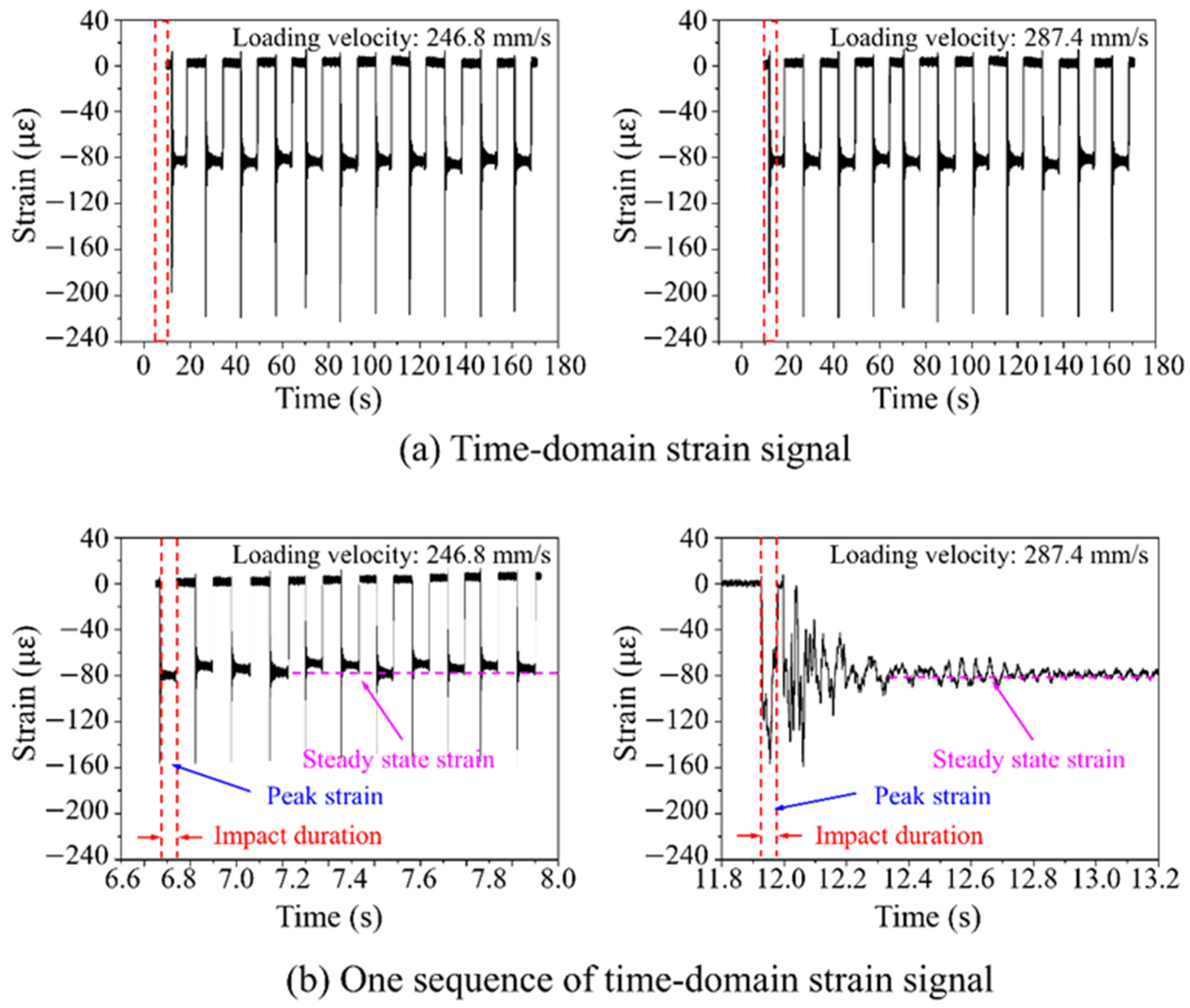
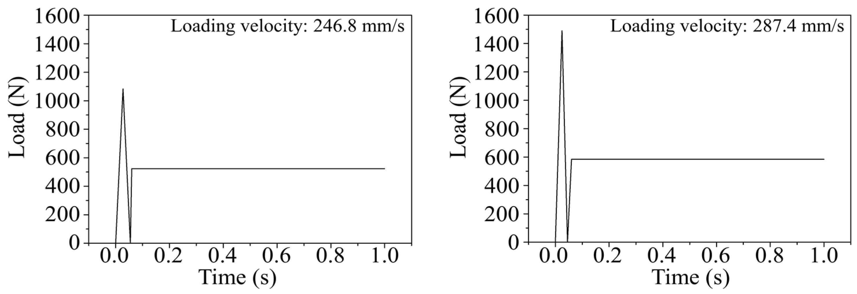
4.2. Reconstruction of Impact Load

The strains measured by the impact load transducer during 11 consecutive impacts under two loading velocities were examined. The time-domain strain signal recorded by the transducer is shown in Figure 7a. Figure 7b shows a sequence of the time-domain strain signals. The important parameters that characterize the measured strain induced by impact are the peak strain, impact duration, and strain in steady state, which is a strain induced by self-weight after impact. In the impact experiment with vehicle chassis, one or two successive peak compressive strain data were obtained because of oscillation. The vibration of a slim and flat vehicle chassis after the first impact causes oscillation of the strain data. The determination method is applied as follows. The peak strain is defined as the first compressive peak strain caused by the impact of the vehicle chassis. The impact duration is defined as the time difference between the two local minimum compressive strain points, which are the points nearest to the first peak compressive strain point. The strain in the steady state is defined by the average strain caused by the vehicle chassis weight after impact. The peak strain, impact duration, and strain in the steady state for the 11 consecutive impacts with two loading velocities are listed in

Table 3. Peak strain, impact duration, and steady state strain measured in 11 sets of experiments for two loading velocities.

	Loading Velocity: 246.8 (mm/s)			Loading Velocity: 287.4 (mm/s)
Set	Peak Strain (με)	Impact Duration (s)	Steady State Strain (με)	Peak Strain (με)	Impact Duration (s)	Steady State Strain (με)
1.	−159.00	0.05378	−79.50	−197.00	0.04953	−81.50
2.	−157.00	0.05566	−74.00	−218.75	0.04213	−82.25
3.	−155.00	0.05664	−77.50	−219.25	0.04259	−83.50
4.	−154.25	0.05518	−70.0	−218.00	0.04200	−80.25
5.	−156.00	0.05810	−71.00	−210.75	0.04199	−82.75
6.	−152.25	0.05469	−78.00	−222.75	0.04249	−84.50
7.	−155.75	0.05615	−70.00	−215.50	0.04248	−82.50
8.	−156.75	0.05811	−74.00	−216.75	0.04199	−82.25
9.	−155.25	0.05420	−71.00	−218.75	0.04200	−85.50
10.	−155.50	0.05469	−71.25	−218.50	0.04199	−81.00
11.	−158.50	0.05468	−74.00	−213.75	0.04248	−83.25
Standard deviation	1.89	0.00148	3.39	6.87	0.00222	1.51
Average	−155.90	0.05630	−73.66	−215.43	0.04288	−82.66

. The average values of the peak strain, impact duration, and strain in the steady state with the loading velocity of 246.8 mm/s are −155.90 με, 0.05630 s, and −73.66 με, respectively, and their standard deviations are 1.89 με, 0.00148 s, and 3.39 με, respectively. Similarly, the average peak strain, impact duration, and strain in the steady state for the experiment with the loading velocity of 287.4 mm/s are −215.43 με, 0.04288 s, and −82.66 με, respectively, and their standard deviations are 6.87 με, 0.00222 s, and 1.51 με, respectively. Thus, the measured values of peak strain, impact duration, and strain in the steady state in each set of experiments are consistent enough to demonstrate the reliability of the impact load transducer.

From the experimental results, we observe that the increased loading velocity results in an increased compressive strain of the impact load transducer, whereas the impact duration is shortened. In addition, there is a difference in strain in the steady state of 9 με between the two loading velocities.

Load curves were reconstructed from the average strain data (the peak compressive strain, impact duration, and strain in the steady state) using our method. The reconstructed impact loads for different loading velocities are shown in Figure 8. According to the reconstructed load curves, the peak load, impact duration, and load in the steady state at the two loading velocities are 1083.90 N/0.05630 s/522.95 N and 1489.95 N/0.04288 s/584.33 N, respectively. The reconstructed impact loads were employed as external forces in the numerical simulations.

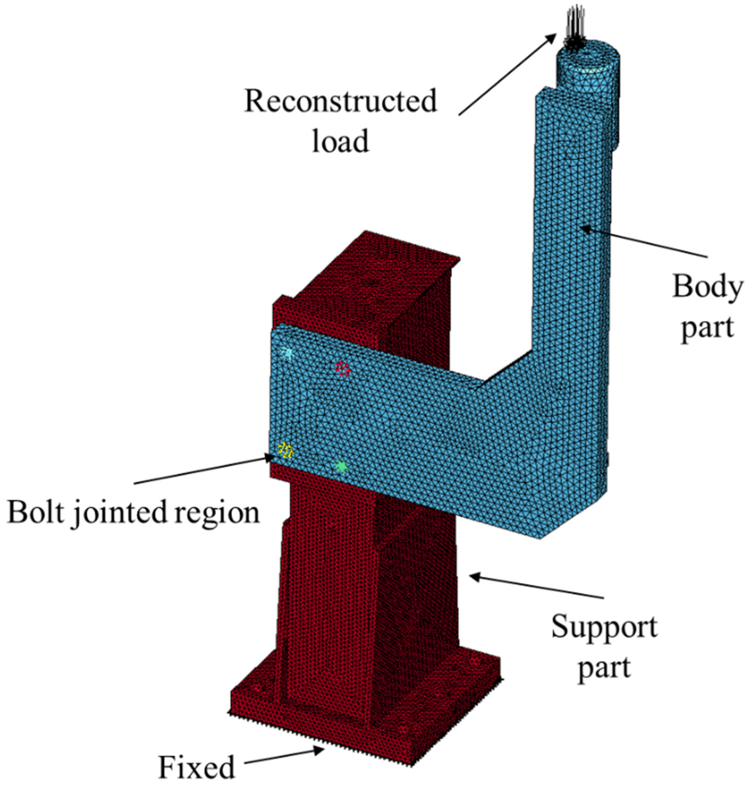
4.3. Numerical Model

The numerical model of the jig structure is presented in Figure 9. Complex features such as round edges and tightening bolts are simplified to enhance the modeling and calculation efficiency. The boundary conditions for the finite element analysis are modeled based on the analysis of the jig structures and vehicle chassis in the production line of Hyundai Motors. A fixed constraint is applied at the bottom of the jig structure, and the bolt-jointed part of the jig structure is modeled as a node-set rigid body. This technique is commonly used as connections between structural parts (particularly in bolt-jointed and welded parts) for efficient simulations. In order to prevent penetration of two body parts during numerical analysis, surface to surface contact is applied on both body and support parts. The reconstructed impact load was applied as a nodal force. The body part and support part of the jig structure, both made of steel, are modeled with an elastic modulus of 210 GPa. Although a simplified model is adopted, the jig structure of the production equipment still displays a complex geometry. A tetrahedron mesh is adopted in this model to incorporate the complex features without compromising on mesh quality.

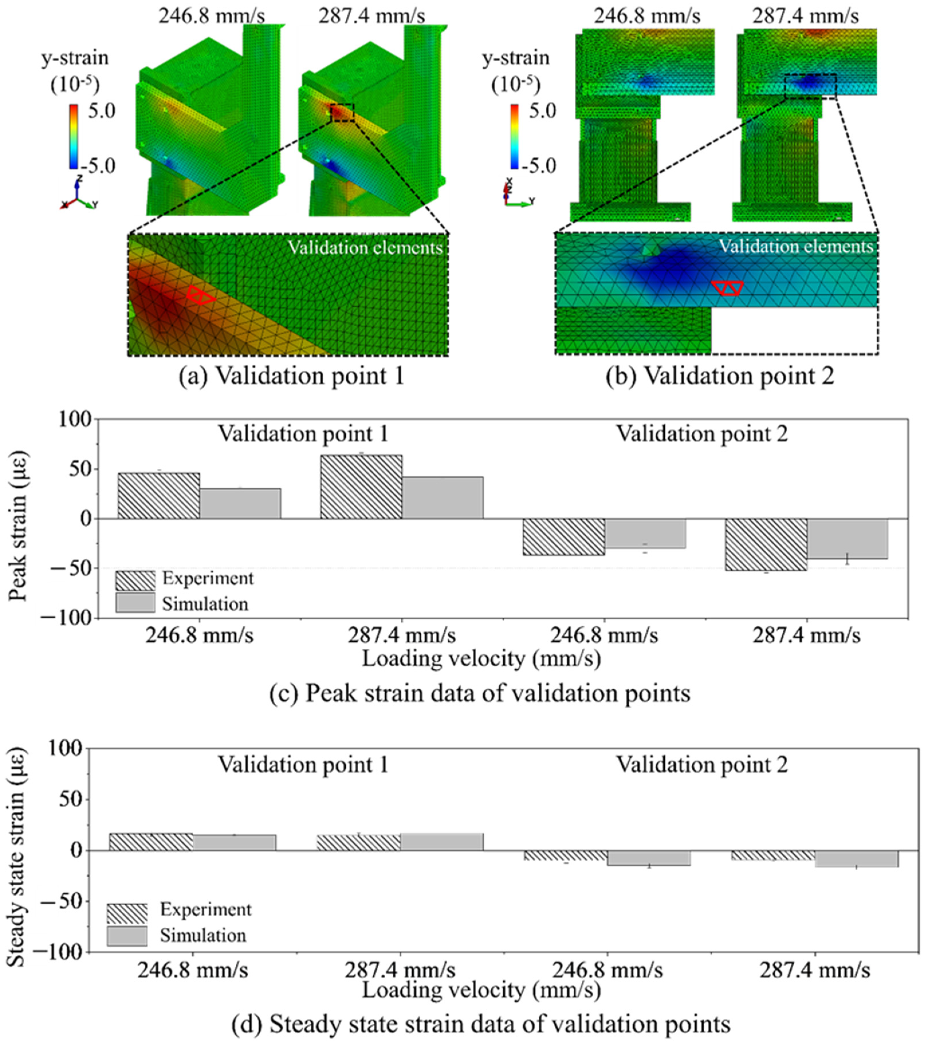
4.4. Validation of Reconstructed Impact Load with Production Equipment

The accuracy of the reconstructed impact load was investigated with the calculated and measured peak strains and the strain in the steady state at the validation points. The impact-induced peak strain and the strain in the steady state were measured at three validation points of the structure in both experiments and numerical simulation, as presented in Figure 10. The strains measured at Validation points 1 and 2 are the y-strain. The y-axis deformation of Validation points 1 and 2 is caused primarily by a bending force induced by the impact. Mainly tension is generated at Validation point 1, whereas compression is generated at Validation point 2. The error bars in the experimental data describe the deviation in the strain data measured during 11 consecutive impacts. The peak strain and the strain in the steady state measured in the experiments are listed in

Table 4. Peak strain of validation points measured in 11 sets of experiments for two loading velocities.

	Loading Velocity: 246.8 (mm/s)			Loading Velocity: 287.4 (mm/s)
Set	Validation Point 1 (με)	Validation Point 2 (με)	Validation Point 3 (με)	Validation Point 1 (με)	Validation Point 2 (με)	Validation Point 3 (με)
1.	45.00	−41.00	−153.00	66.00	−54.00	−212.00
2.	44.00	−39.00	−150.00	64.00	−54.00	−215.00
3.	44.00	−38.00	−150.00	65.00	−52.00	−210.00
4.	44.00	−39.00	−150.00	64.00	−53.00	−211.00
5.	45.00	−38.00	−150.00	62.00	−55.00	−210.00
6.	45.00	−38.00	−149.00	65.00	−51.00	−208.00
7.	46.00	−38.00	−148.00	66.00	−50.00	−207.00
8.	45.00	−36.00	−148.00	64.00	−52.00	−209.00
9.	49.00	−34.00	−145.00	63.00	−52.00	−210.00
10.	49.00	−32.00	−143.00	62.00	−50.00	−208.00
11.	49.00	−32.00	−146.00	62.00	−52.00	−206.00
Standard deviation	2.07	2.96	2.80	1.51	1.62	2.50
Average	45.91	−36.82	−148.36	63.91	−52.27	−209.64

and

Table 5. Steady state strain of validation points measured in 11 sets of experiments for two loading velocities.

	Loading Velocity: 246.8 (mm/s)			Loading Velocity: 287.4 (mm/s)
Set	Validation Point 1 (με)	Validation Point 2 (με)	Validation Point 3 (με)	Validation Point 1 (με)	Validation Point 2 (με)	Validation Point 3 (με)
1.	15.00	−12.00	−47.00	17.00	−11.00	−46.00
2.	14.00	−11.00	−45.00	16.00	−10.00	−43.00
3.	15.00	−11.00	−45.00	15.00	−10.00	−43.00
4.	15.00	−11.00	−45.00	15.00	−10.00	−42.00
5.	15.00	−10.00	−43.00	15.00	−9.00	−42.00
6.	16.00	−10.00	−44.00	15.00	−9.00	−42.00
7.	17.00	−11.00	−45.00	14.00	−9.00	−41.00
8.	18.00	−9.00	−41.00	15.00	−8.00	−40.00
9.	19.00	−8.00	−42.00	14.00	−8.00	−42.00
10.	18.00	−7.00	−40.00	13.00	−9.00	−41.00
11.	19.00	−7.00	−41.00	13.00	−8.00	−41.00
Standard deviation	1.81	1.74	2.21	1.19	0.98	1.58
Average	16.45	−9.73	−43.45	14.73	−9.18	−42.09

. The error bars in the numerical simulation are presented to illustrate the uncertainty of the validation positions with respect to those in the experiments. Three elements selected at each validation point are shown in Figure 10a,b. The average peak strain and the strain in the steady state at each validation point are shown in Figure 10c. The average peak strain measured at each validation point for the loading velocity of 246.8 mm/s are 45.09 and −36.82 με, respectively whereas the calculated values are 30.47 and −30.00 με, respectively. The average peak strain measured at each validation point for the loading velocity of 287.4 mm/s are 63.91, −52.27, and −209.63 με, respectively, whereas the calculated values are 41.97, −40.27, and −151.33 με, respectively. The maximum difference between experimentally measured and numerically calculated peak strain is 21.94 με which is at Validation point 1 for the loading velocity of 287.4 mm/s. The distribution of peak strains calculated for the validation points is consistent with those measured in the experiments. Although reasonable, the difference in magnitude of peak strain can be reduced by a more sophisticated simulation model of the jig structure with refined tightening bolts and complex features (these had been simplified in this study for computational efficiency).

The average strain in the steady state measured at each validation point for the loading velocity of 246.8 mm/s are 16.46 and −9.73 με, respectively, whereas the calculated values are 15.07 and −14.97 με, respectively. The average strain in the steady state measured at each validation point for the loading velocity of 287.4 mm/s are 14.73 and −9.18 με, respectively whereas the calculated values are 16.67 and −16.57 με, respectively. The strain in the steady state is caused mainly by the vehicle chassis weight and is consistent regardless of the loading velocity.

The unknown external impact was determined and validated through experiments on the production equipment. Impact-induced structural strains were predicted with good accuracy by applying the reconstructed impact load in the numerical simulation. These results reveal that the proposed method for determining impact loads can be applied to predict the impact response of production equipment in various fields.

5. Conclusions

The outcome of this study verifies the accuracy of the proposed method in determining externally applied impact loads on complex production equipment. The peak strain, impact duration, and strain in steady state were accurately measured by a newly designed transducer incorporating strain gauges. The measured strain gauge signals were converted by the developed conversion model to the impact load curve that characterizes impact peak force, impact duration, and load in the steady state after impact. To validate the method for determining impact load, the reconstructed impact loads were employed in numerical simulations, and the numerically calculated structural strains were compared with those measured in the experiments. The maximum difference in structural peak strain at the validation points for the lab-scale impact experiments and production line impact experiments are 3.2 and 21.94 με respectively, even with the simplified model of the jig structure. The results indicate that the proposed method can determine externally applied impact loads with sufficient accuracy. Furthermore, the reconstructed load curve obtained using the developed method provides high efficiency in addition to high accuracy without the complexities of modeling dynamic impact simulation (including complex impactor shape, interface, and friction conditions). Therefore, this research provides a convenient method to predict externally applied impact loads and enables the further study of structural behavior in various fields such as stress–strain analysis, fatigue analysis, and topology optimization for lightweight design of production equipment.

References

1. Fan, J.; Njuguna, J. An introduction to lightweight composite materials and their use in transport structures. In Lightweight Composite Structures in Transport; Njuguna, J., Ed.; Woodhead Publishing: Amsterdam, The Netherlands, 2016; pp. 3–34. [Google Scholar]
2. Batista, M.D.R.; Drzal, L.T.; Kiziltas, A.; Mielewski, D. Hybrid cellulose-inorganic reinforcement polypropylene composites: Lightweight materials for automotive applications. Polym. Compos. 2020, 41, 1074–1089. [Google Scholar] [CrossRef]
3. Peng, X.; Sui, Y. Lightweight topology optimization with consideration of the fail-safe design principle for continuum structures. Eng. Optim. 2021, 53, 32–48. [Google Scholar] [CrossRef]
4. Li, J.; Wang, D. Study on application of MSOT method for lightweight design of automobile body structure. Adv. Mech. Eng. 2020, 12, 1687814020965049. [Google Scholar]
5. Zhao, H.; Wang, R.; Li, Q.M.; Wu, H.; Hou, C.-C.; An, G. Experimental and numerical investigation on impact and post-impact behaviours of H-shaped steel members. Eng. Struct. 2020, 216, 110750. [Google Scholar] [CrossRef]
6. Ince, S.T.; Kumar, A.; Park, D.K.; Paik, J.K. An advanced technology for structural crashworthiness analysis of a ship colliding with an ice-ridge: Numerical modelling and experiments. Int. J. Impact Eng. 2017, 110, 112–122. [Google Scholar] [CrossRef]
7. Khan, M.R.; Sonawane, A. Prediction of impact response in construction safety helmet using FEA. J. Eng. Des. Technol. 2019, 18, 557–566. [Google Scholar] [CrossRef]
8. Kishi, N.; Ohno, T.; Konno, H.; Bhatti, A.Q. Dynamic Response Analysis for a Large-scale RC Girder Under a Falling-weight Impact Loading. Adv. Eng. Struct. Mech. Const. 2006, 140, 99–109. [Google Scholar]
9. Gilardi, G.; Sharf, I. Literature survey of contact dynamics modelling. Mech. Mach. Theory 2002, 37, 1213–1239. [Google Scholar] [CrossRef]
10. Kurşun, A.; Şenel, M.; Enginsoy, H.M.; Bayraktar, E. Effect of impactor shapes on the low velocity impact damage of sandwich composite plate: Experimental study and modelling. Compos. B Eng. 2016, 86, 143–151. [Google Scholar] [CrossRef]
11. Jacquelin, E.; Hamelin, P. Force recovered from three recorded strains. Int. J. Solids Struct. 2003, 40, 73–88. [Google Scholar] [CrossRef]
12. Hu, N.; Fukunaga, H.; Matsumoto, S.; Yan, B.; Peng, X.H. An efficient approach for identifying impact force using embedded piezoelectric sensors. Int. J. Impact Eng. 2007, 34, 1258–1271. [Google Scholar] [CrossRef]
13. Qiao, B.; Zhang, X.; Gao, J.; Chen, X. Impact-force sparse reconstruction from highly incomplete and inaccurate measurements. J. Sound Vib. 2016, 376, 72–94. [Google Scholar] [CrossRef]
14. Sun, L.; Li, Y.; Zhu, W.; Zhang, W. Structural response reconstruction in physical coordinate from deficient measurements. Eng. Struct. 2020, 212, 110484. [Google Scholar] [CrossRef]
15. Law, S.S.; Chan, T.H.T.; Zeng, Q.H. Moving Force Identification: A Time Domain Method. J. Sound Vib. 1997, 201, 1–22. [Google Scholar] [CrossRef]
16. Vyas, N.S.; Wicks, A.L. Reconstruction of turbine blade forces from response data. Mech. Mach. Theory 2001, 36, 177–188. [Google Scholar] [CrossRef]
17. Jacquelin, E.; Bennani, A.; Hamelin, P. Force reconstruction: Analysis and regularization of a deconvolution problem. J. Sound Vib. 2003, 265, 81–107. [Google Scholar] [CrossRef]
18. Kim, S.J.; Lee, S.W. Experimental identification for inverse problem of a mechanical system with a non-minimum phase based on singular value decomposition. J. Mech. Sci. Technol. 2008, 22, 1504–1509. [Google Scholar] [CrossRef]
19. Qiao, B.; Chen, X.; Xue, X.; Luo, X.; Liu, R. The application of cubic B-spline collocation method in impact force identification. Mech. Syst. Signal Process. 2015, 64, 413–427. [Google Scholar] [CrossRef]
20. Gunawan, F.E. Levenberg–Marquardt iterative regularization for the pulse-type impact-force reconstruction. J. Sound Vib. 2012, 331, 5424–5434. [Google Scholar] [CrossRef]
21. Ma, C.-K.; Chang, J.-M.; Lin, D.-C. Input Forces Estimation of Beam Structures by an Inverse Method. J. Sound Vib. 2003, 259, 387–407. [Google Scholar] [CrossRef]
22. De Simone, M.E.; Ciampa, F.; Meo, M. A hierarchical method for the impact force reconstruction in composite structures. Smart Mater. Struct. 2019, 28, 085022. [Google Scholar] [CrossRef]
23. Akhavan, F.; Watkins, S.; Chandrashekhara, K. Prediction of Impact Contact Forces of Composite Plates Using Fiber Optic Sensors and Neural Networks. Mech. Adv. Mater. Struct. 2000, 7, 195–205. [Google Scholar] [CrossRef]
24. Yuan, F.-G.; Zargar, S.A.; Chen, Q.; Wang, S. Machine learning for structural health monitoring: Challenges and opportunities. In Proceedings of SPIE 11379, Sensors and Smart Structures Technologies for Civil, Mechanical, and Aerospace Systems 2020; SPIE: Bellingham, WA, USA, 2020; p. 1137903. [Google Scholar]
25. Zargar, S.A.; Yuan, F.-G. Impact diagnosis in stiffened structural panels using a deep learning approach. Struct. Health Monit. 2021, 20, 681–691. [Google Scholar] [CrossRef]
26. Ganeshan, V.; Dattakumar, S.S. Converting Dynamic Impact Events to Equivalent Static Loads in Vehicle Chassis. Master’s Thesis, Chalmers University of Technology, Gothenburg, Sweden, 2017. [Google Scholar]
Figure 1. Illustration of method to identify the external impact load acting on production equipment. (a) Schematic of process for determining impact load and application of reconstructed impact load; (b) procedure for calibrating impact load transducer using uniaxial compression test; (c) model for conversion from strain signal to impact load.
Applsci 12 02870 g001
Figure 2. Experimental set-up. (a) Experimental set-up for measuring transducer and structural strain due to impact; (b) structure installed with impact load transducer and strain gauges (y-axis) for validation.
Applsci 12 02870 g002
Figure 3. Results of impact experiments. (a) Time-domain strain signal of impact load transducer with 10 consecutive impacts; (b) a sequence of time-domain strain signal.
Applsci 12 02870 g003
Figure 4. Reconstructed impact loads.
Applsci 12 02870 g004
Figure 5. Validation of reconstructed impact load. (a) Contour representations of y-axis strain distribution with validation elements of Validation point 1; (b) contour representations of y-axis strain distribution with validation elements of Validation point 2; (c) comparison of experimentally measured and numerically calculated peak strain values.
Applsci 12 02870 g005
Figure 6. Illustration of impact experiment in Hyundai Motors production line. (a) Jig structures and vehicle chassis; (b) jig structure installed with impact load transducer and strain gauges; (c) impact load transducer mounted on impact point; (d,e) strain gauges attached to the stress concentration region for validating FE simulation.
Applsci 12 02870 g006
Figure 7. Results of impact experiments. (a) Time-domain strain signal measured by impact load transducer during 11 consecutive impacts; (b) a sequence of time-domain strain signal.
Applsci 12 02870 g007
Figure 8. Reconstructed load curves.
Applsci 12 02870 g008
Figure 9. Finite element model of production equipment.
Applsci 12 02870 g009
Figure 10. Validation of reconstructed impact load with production equipment. (a) Contour representations of y-axis strain distribution with validation elements of Validation point 1; (b) contour representations of y-axis strain distribution with validation elements of Validation point 2; (c) comparison of experimentally measured and numerically calculated peak strain; (d) comparison of experimentally measured and numerically calculated strain in steady state.
Applsci 12 02870 g010