
Design and Validation of a Low-Cost Structural Health Monitoring System for Dynamic Characterization of Structures


Abstract
:1. Introduction
2. Background
2.1. Structural Health Monitoring
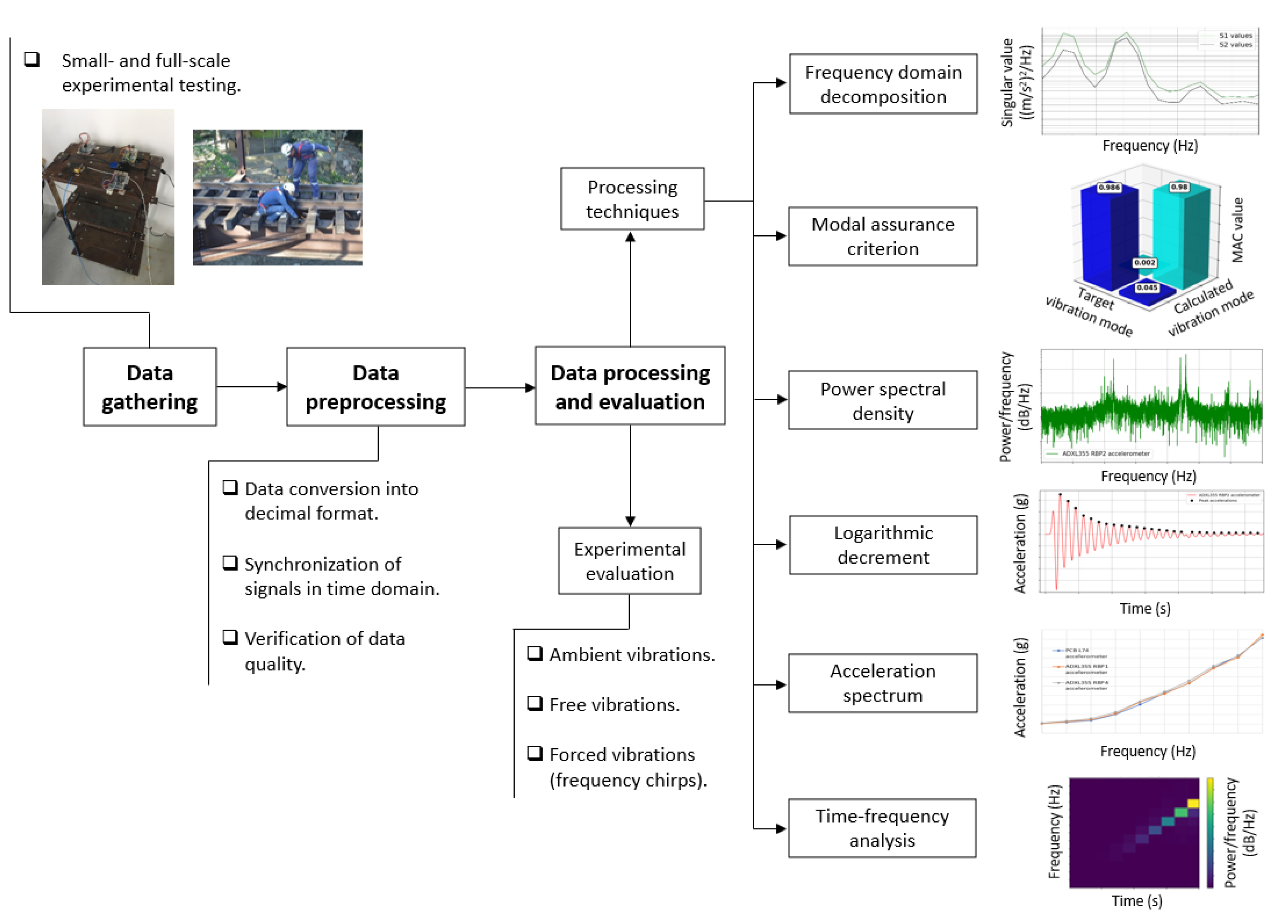
2.2. Dynamic Characterization and Processing Techniques
3. Methodology
3.1. Structural Health Monitoring Systems
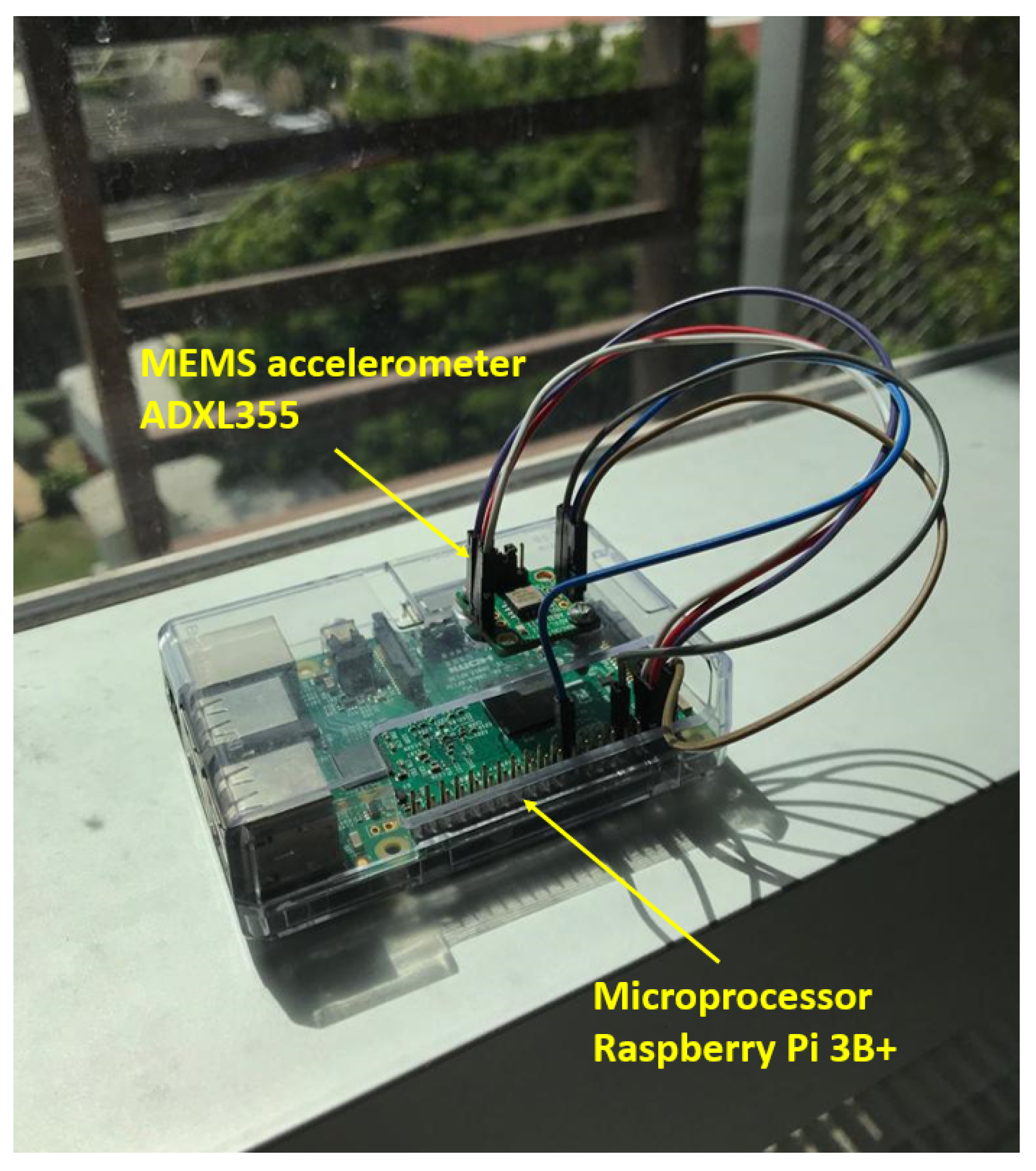
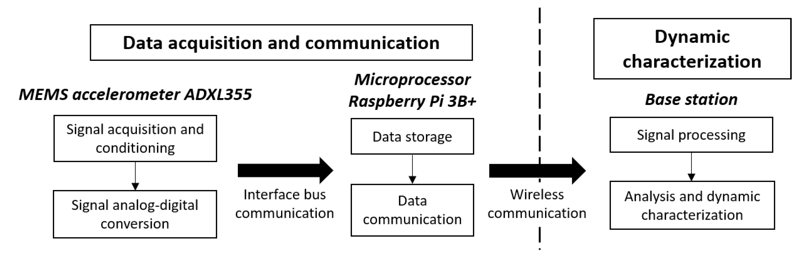
3.1.1. Low-Cost Structural Health Monitoring System
3.1.2. Reference Structural Health Monitoring System
3.2. Descriptions of the Tests
3.2.1. Small-Scale Testing
- –
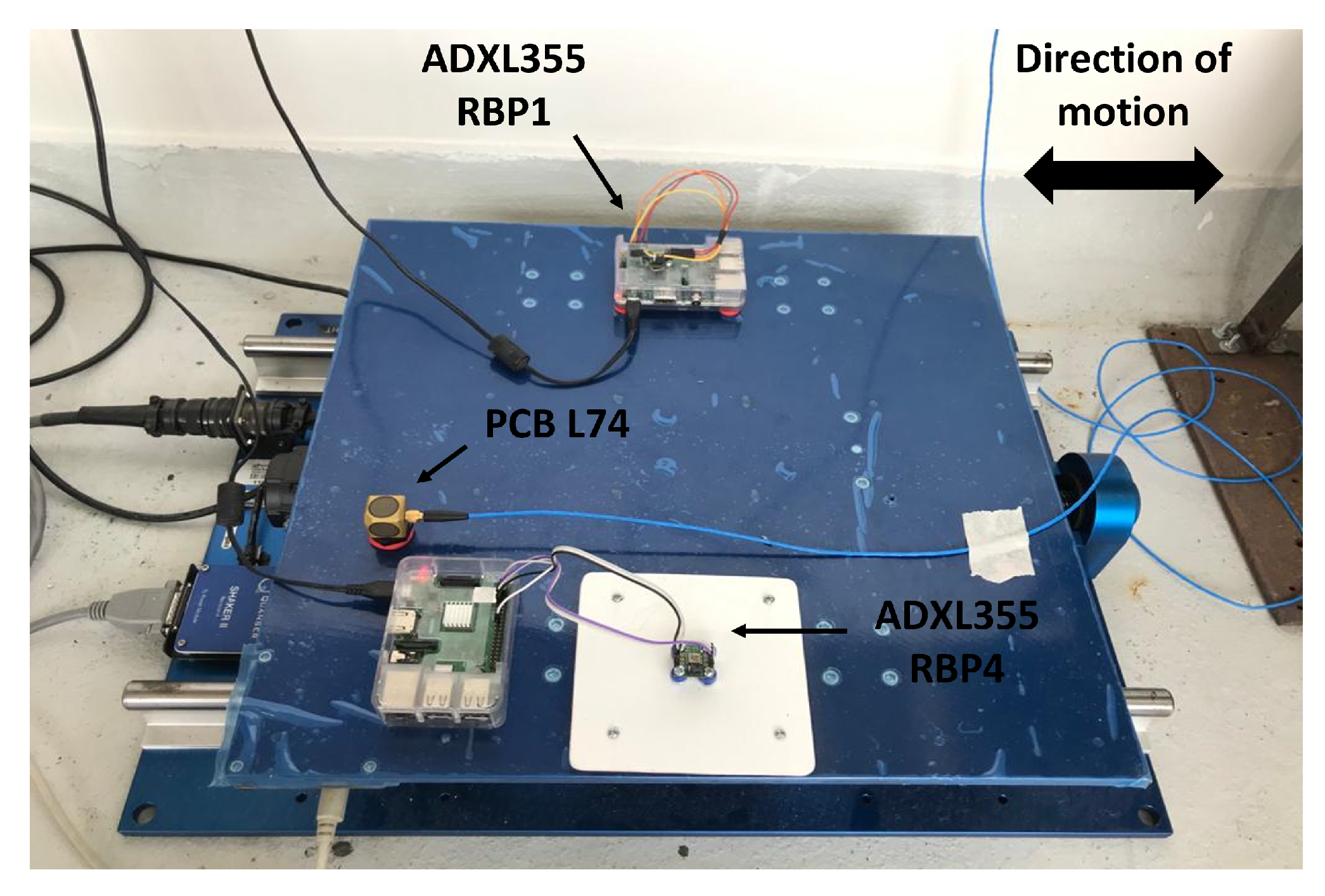
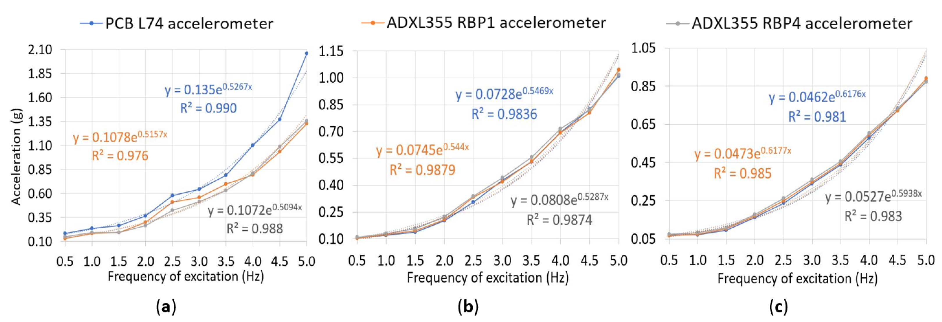
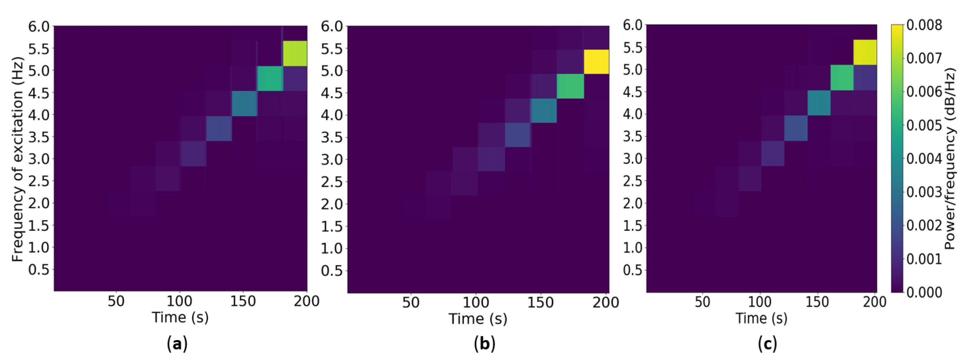
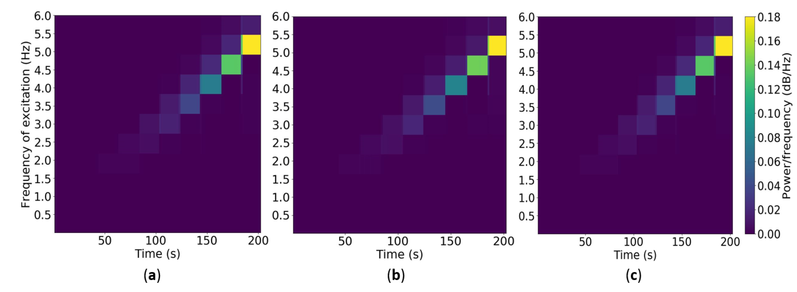
- Shaking Table Tests: The Quanser Shake Table II is a single-axis motion simulator operated with open architecture software. The shaking table can reproduce sinusoidal and frequency chirp motions and pre-loaded accelerograms of real earthquakes employing a plan dimension platform of 61 × 46 cm with a total height of 13 cm. The simulator allows an operational weight of 7.5 kg for an acceleration of 2.5 g [32]. This test ensued in the analysis of data vibrations recorded from frequency chirps performed by the shaking table with different displacements according to distinct frequencies from 0.5 to 5.0 Hz, 0.5 Hz increments, using a sinusoidal excitation. For the frequency chirps, 0.10 cm, 0.25 cm, 0.50 cm, and 0.75 cm displacements were considered. Two wireless measuring nodes and one piezoelectric accelerometer were used to deploy the low-cost and reference SHM systems during testing. The accelerometer arrangement over the Shake Table II platform is presented in Figure 4.
- –
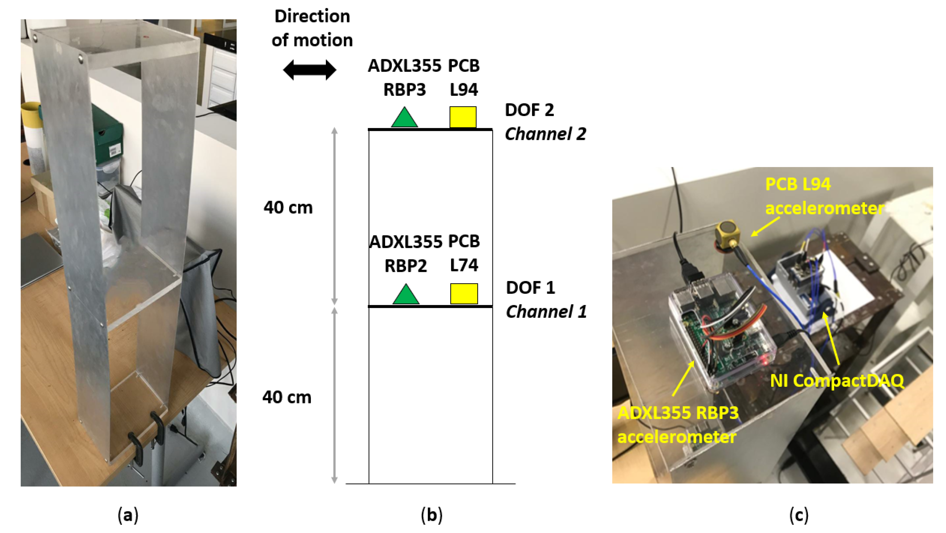
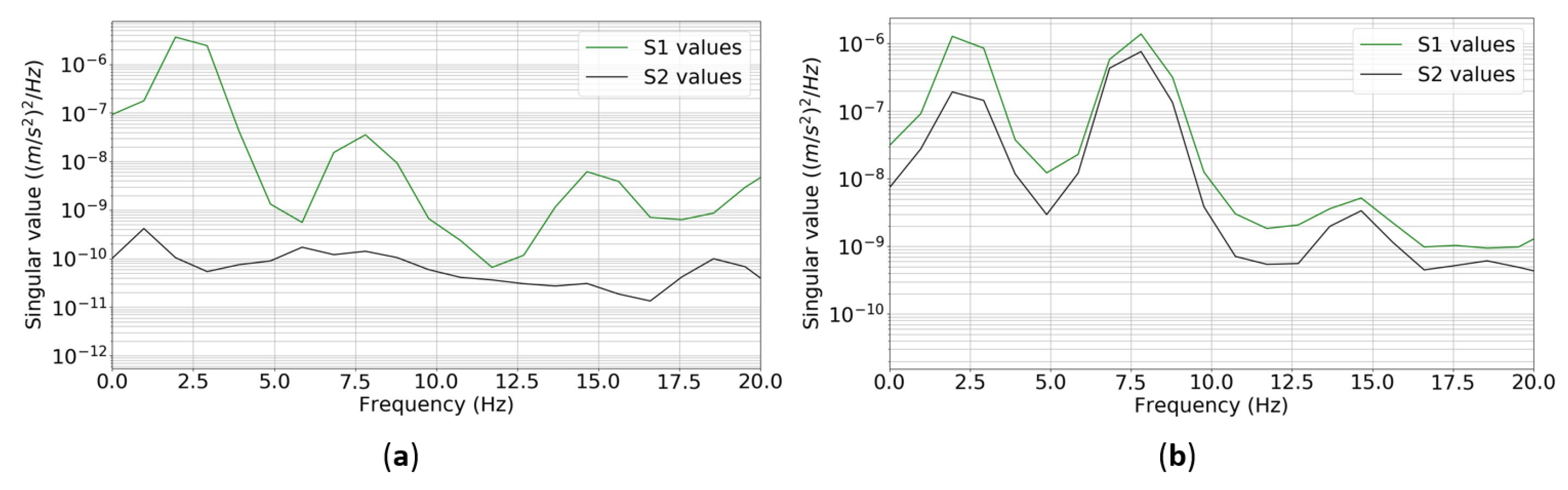
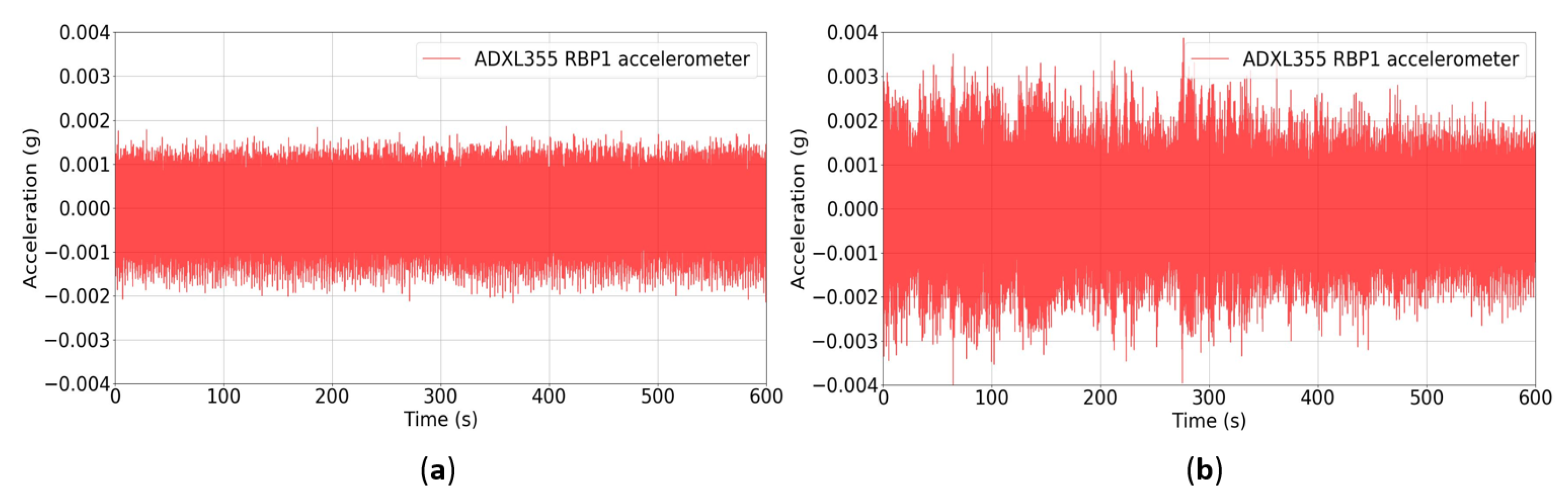
- Flexible Structure Monitoring: The tested two-story structure consists of 15 × 10 cm acrylic plates as floor systems and 80-cm aluminum leaves as lateral support elements. The story height is 40 cm, and the structure was constrained at the bottom above a stiff desk by clamps. The flexible structure was represented as a two-degree-of-freedom (2-DOF) shear frame for the testing. The dynamic characterization of the structure was carried out through ambient and free-vibration records from the structural response, excited by random displacements on the highest DOF. The experimental setup involved a measurement channel on every DOF, and every measurement channel had a measuring unit for each SHM system. Figure 5 shows the aluminum structure, the experimental scheme of the testing, and the sensor array on DOF 2 of the flexible structure.
3.2.2. Full-Scale Testing
- –
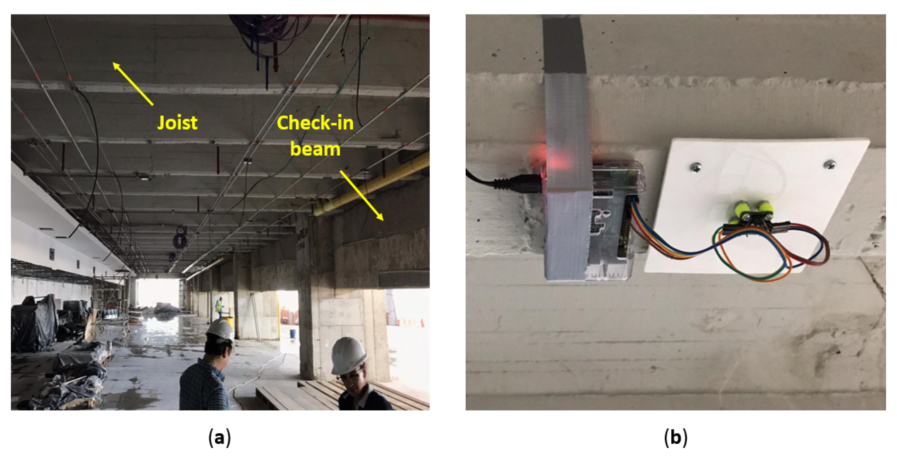
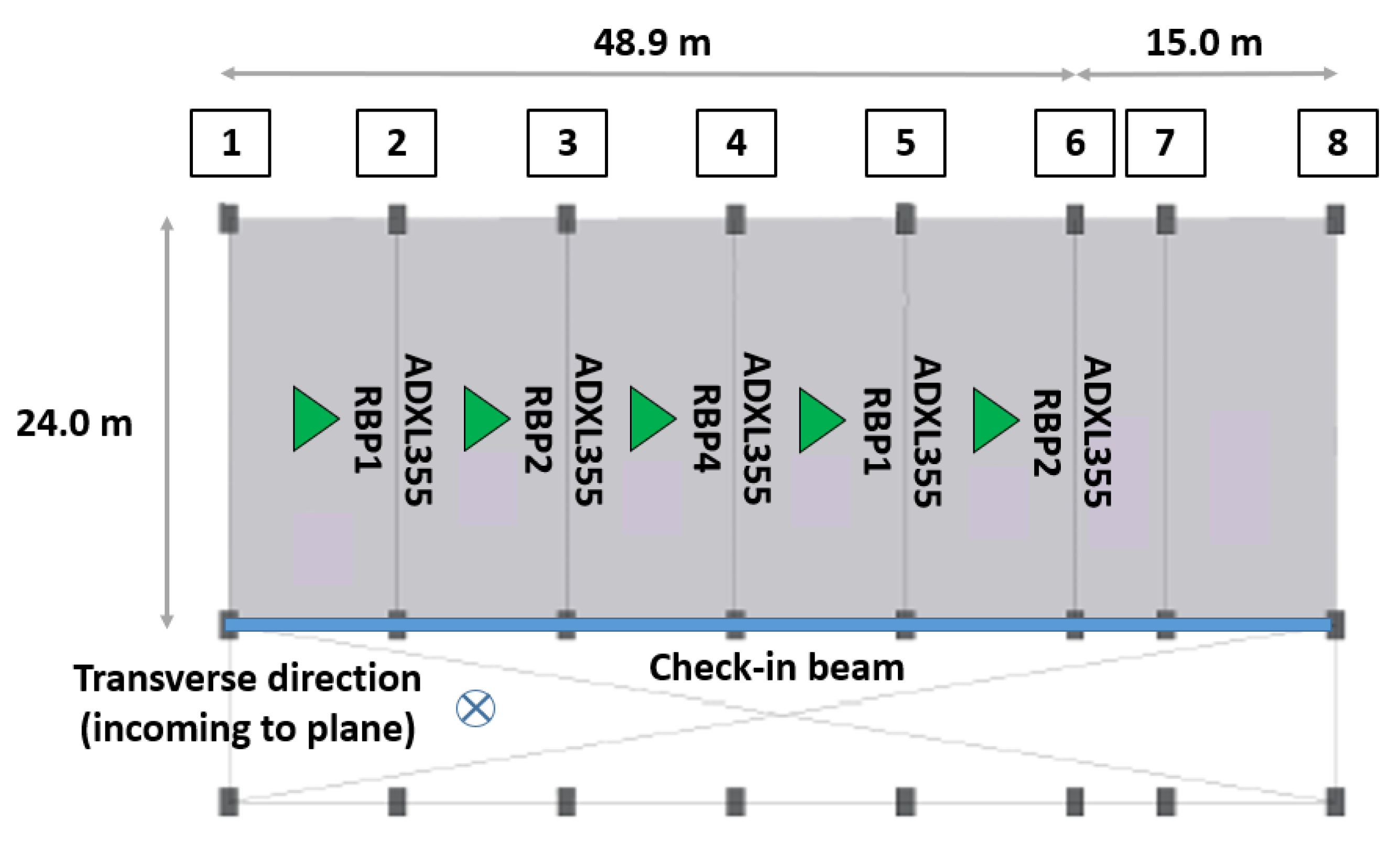
- Beam Demolition Monitoring: The reinforced concrete (RC) beam (later demolished), or so-called check-in beam, was a lateral support element of a lightweight RC slab. The prestressed concrete slab has five primary spans of 24-m joists placed in the lightweight RC slab transverse direction. The 49-m check-in beam supported 30 prestressed concrete joists. Prior to the demolition work, an RC girder was constructed to resist the lightweight RC slab laterally and replace the check-in beam. The prestressed concrete slab was monitored to evaluate whether the vibrations of the demolition would produce significant disturbances to the current service zone of the airport, and thus identify the stiffness changes that may compromise the stability of the structure. The SHM strategy was carried out on the central joist, for each span, through ambient and forced vibration records during the TE 1500-AVR Hilti demolition hammer operation, whose impact frequency was 1620 impacts/minute (27.0 Hz) [33]. A measuring node was installed at the base of the central joist mid-length to every span (Figure 6). The demolition work and structural monitoring were completed at once, span by span, as pointed in Figure 7. Thus, the base station moved continuously throughout the check-in beam demolition.
- –
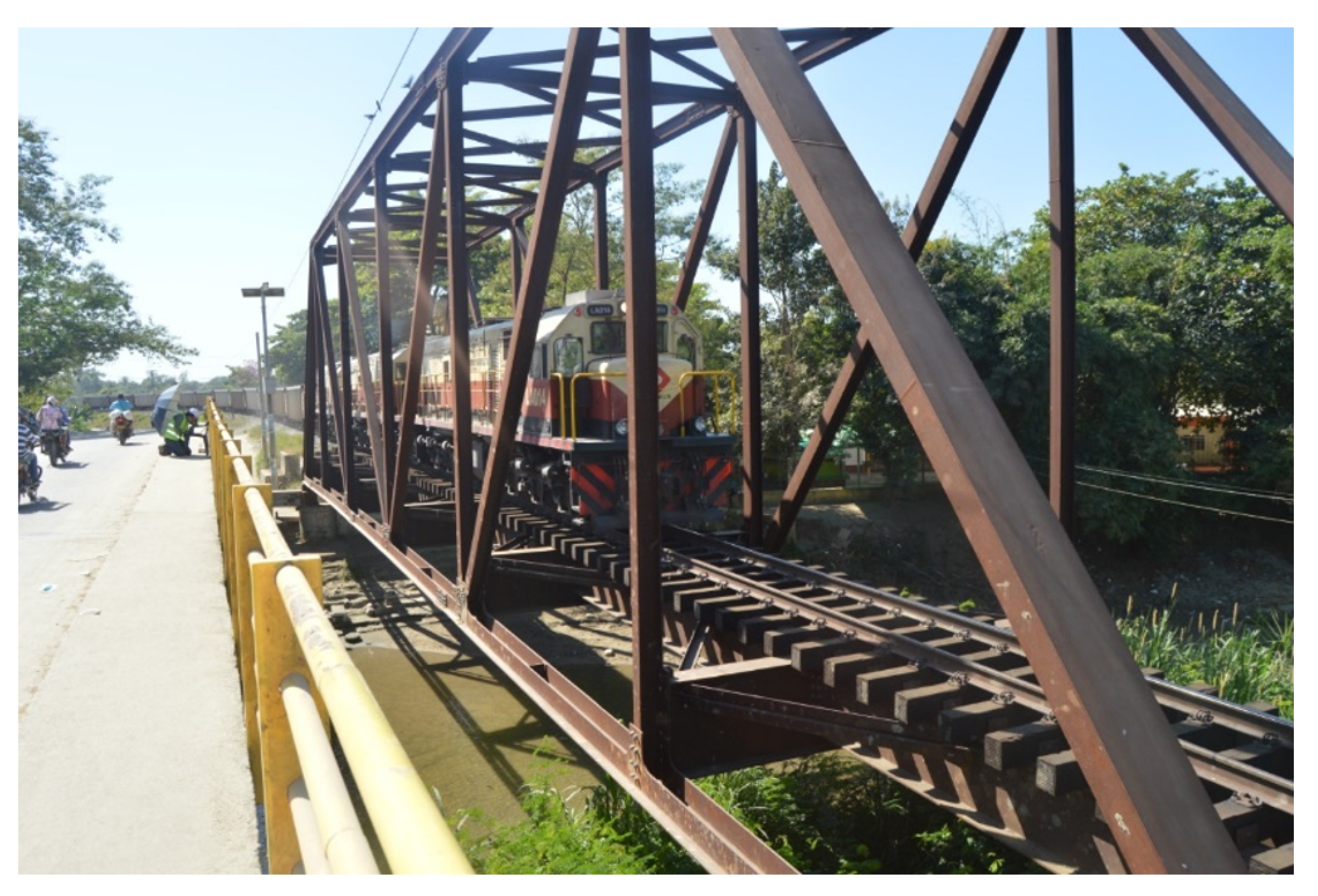
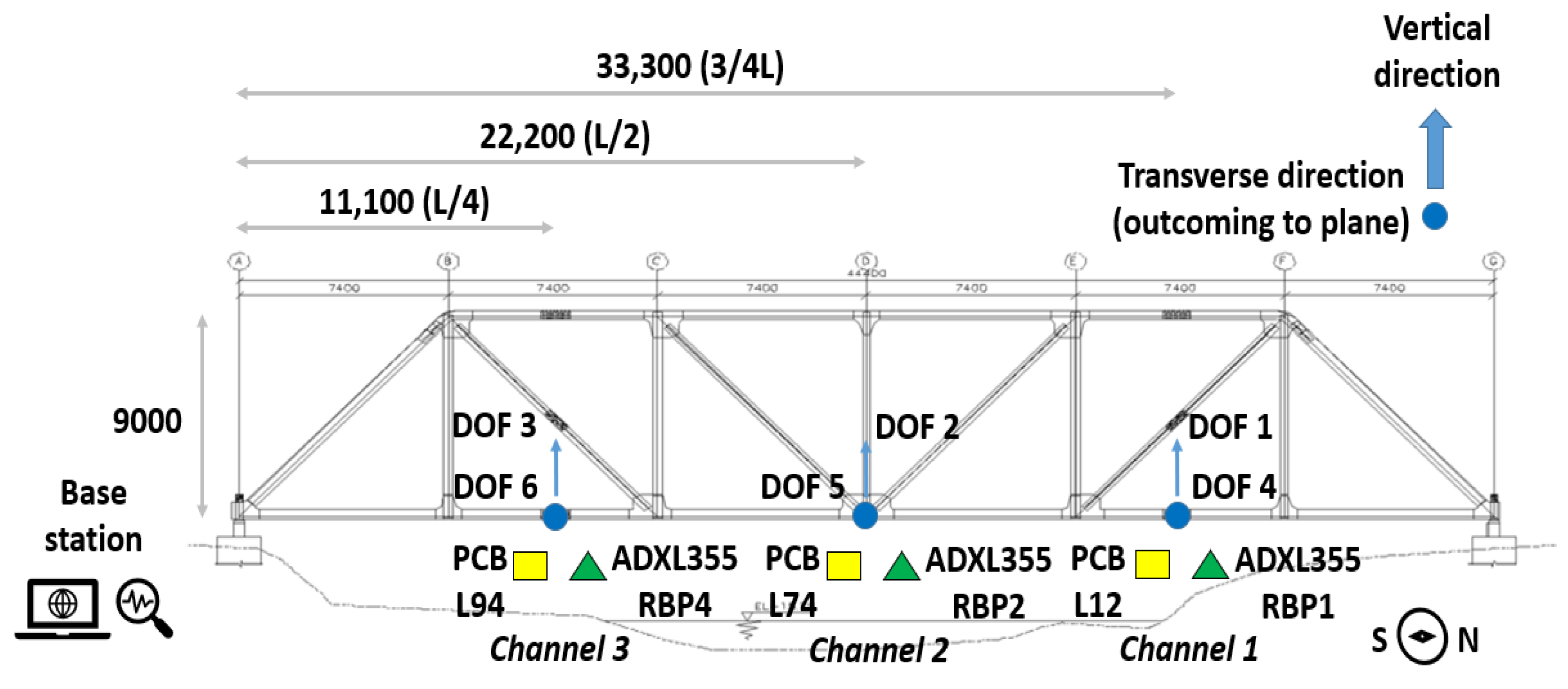
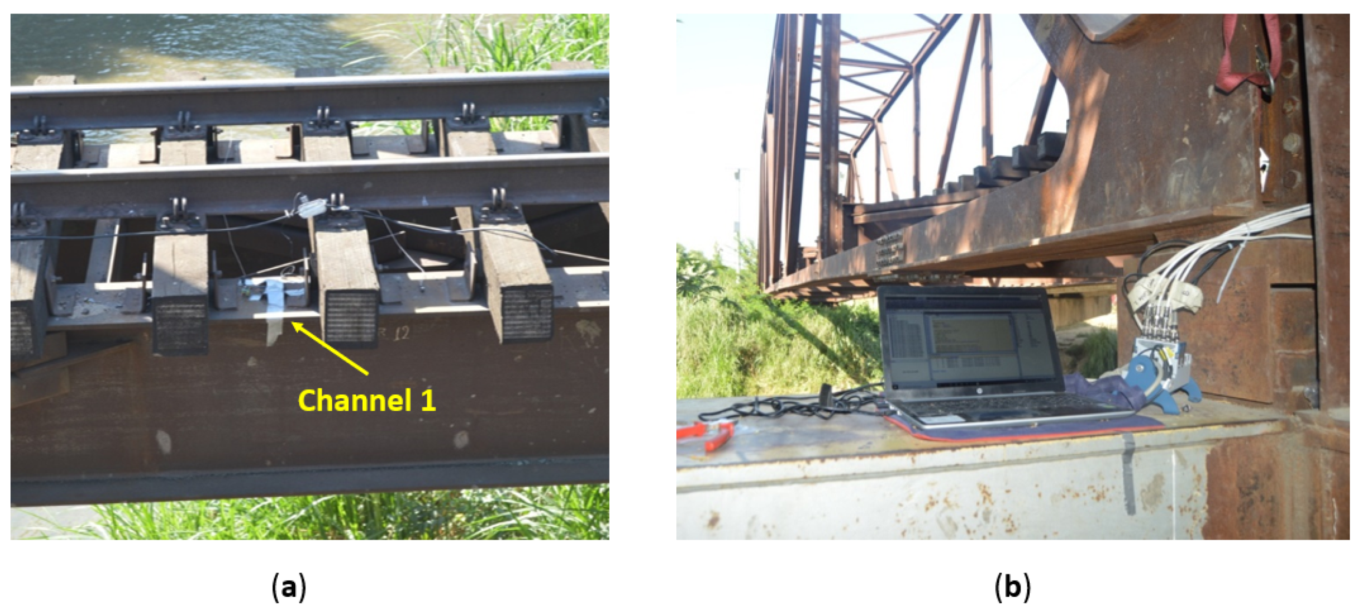
- Railway Bridge Monitoring: The test bridge is a single-span steel structure composed of a tridimensional truss, connected along the top seam by a latticework and along the bottom seam by structural steel members. The steel structure has one 44.0-m span in the longitudinal direction, a deck width of 5.3 m, and a height of 9.0 m. Figure 8 presents a perspective image of the steel structure.
4. Results and Validation
4.1. Small-Scale Testing
4.1.1. Shaking Table Tests
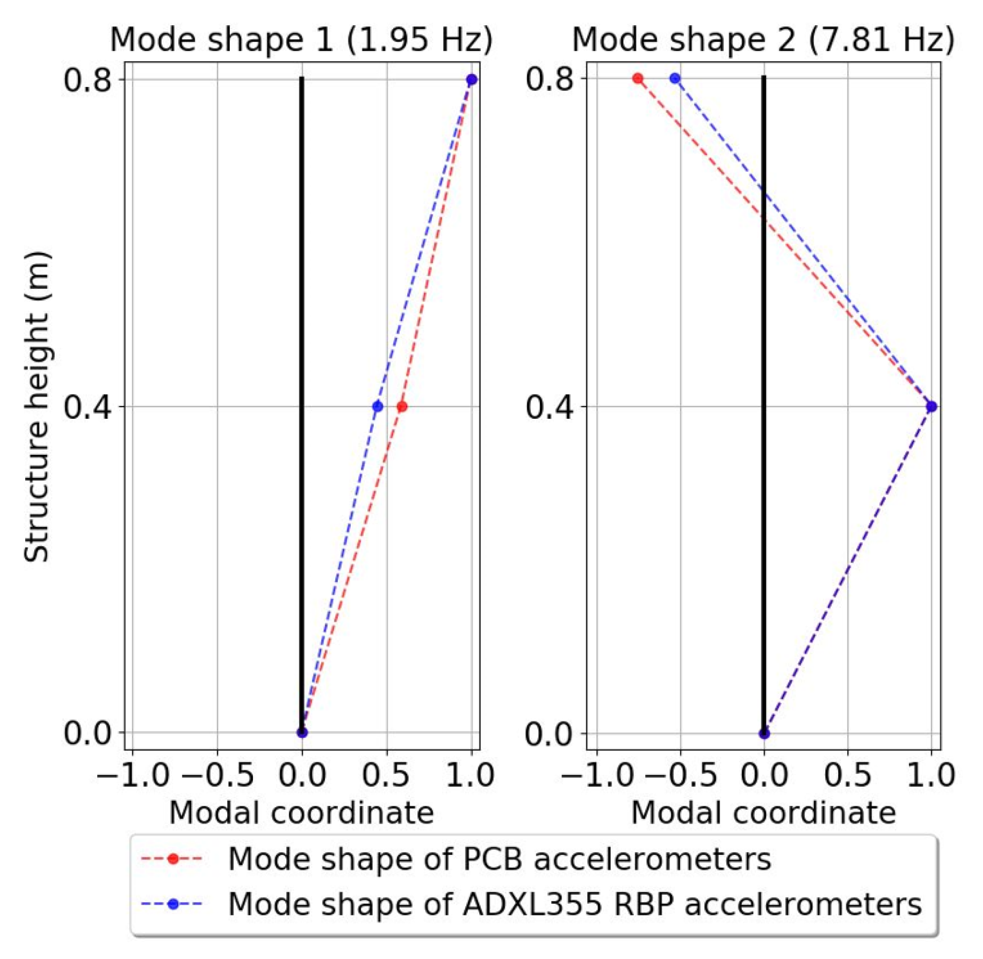
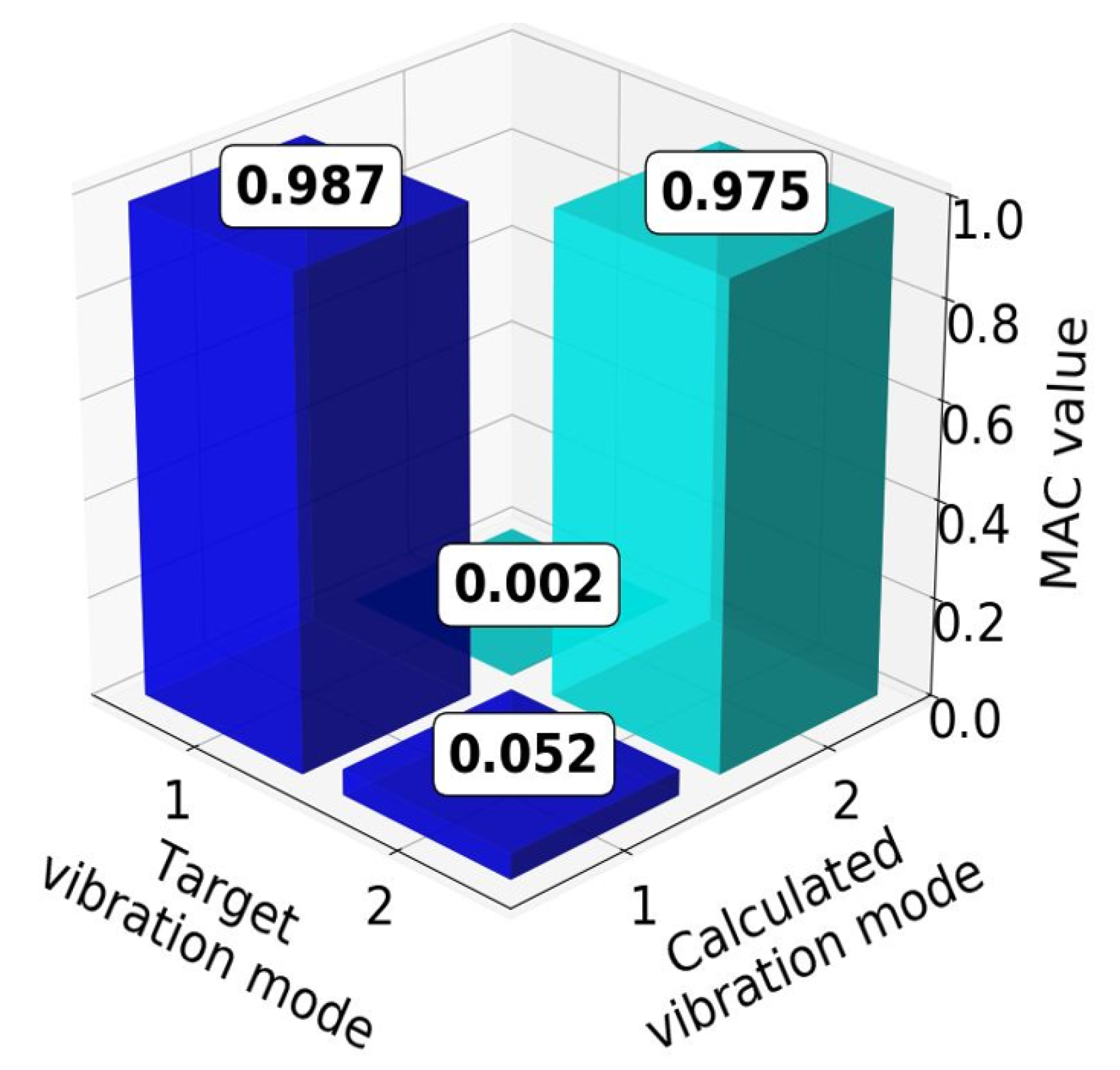
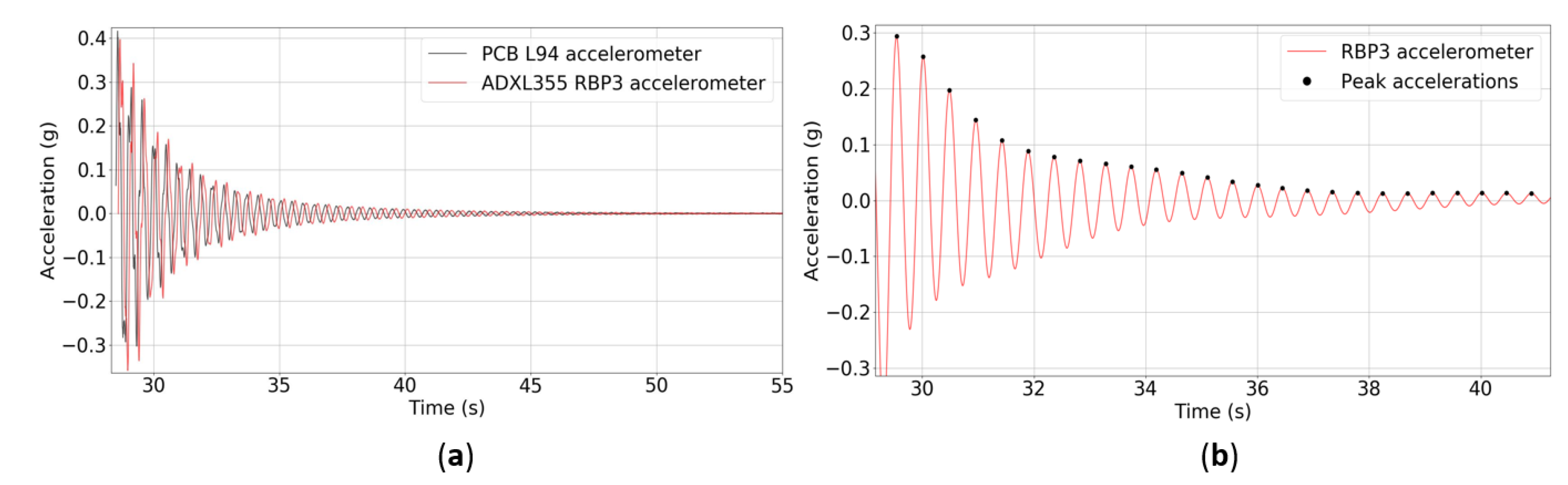
4.1.2. Flexible Structure Monitoring
4.2. Full-Scale Testing
4.2.1. Beam Demolition Monitoring
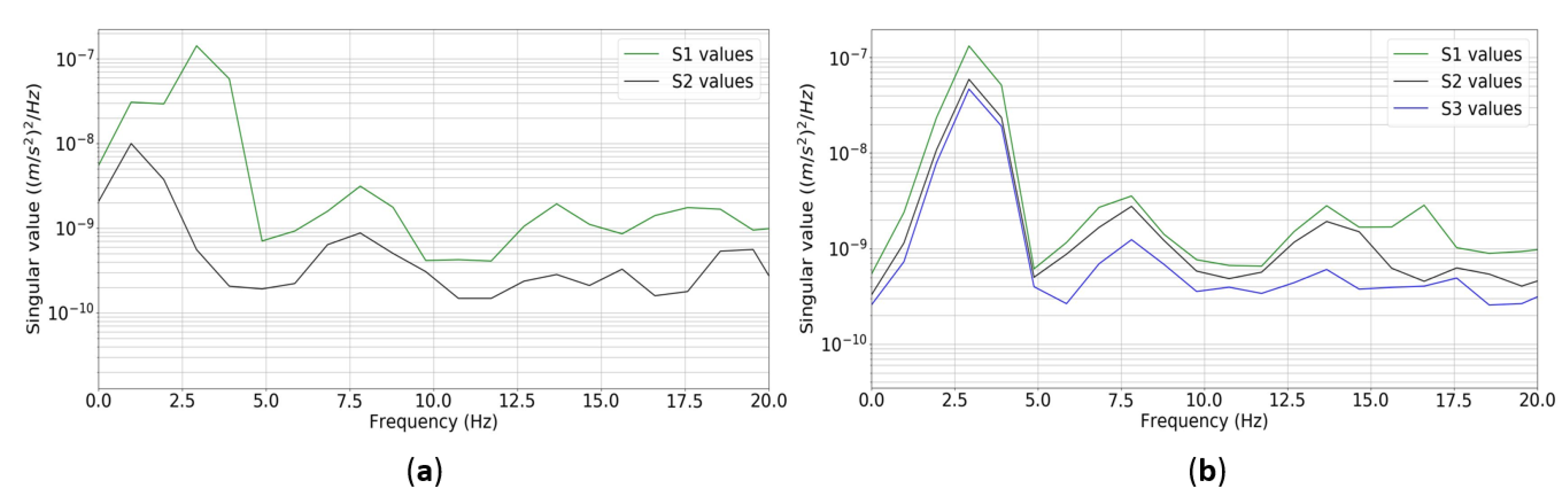
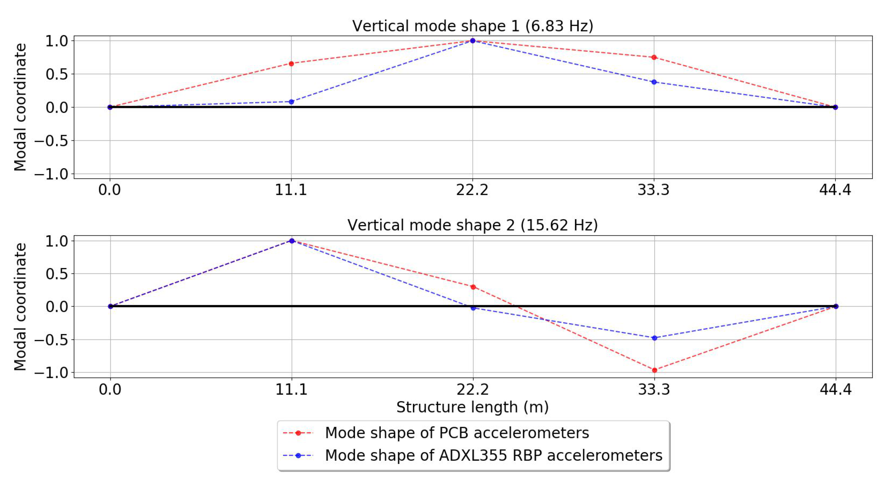
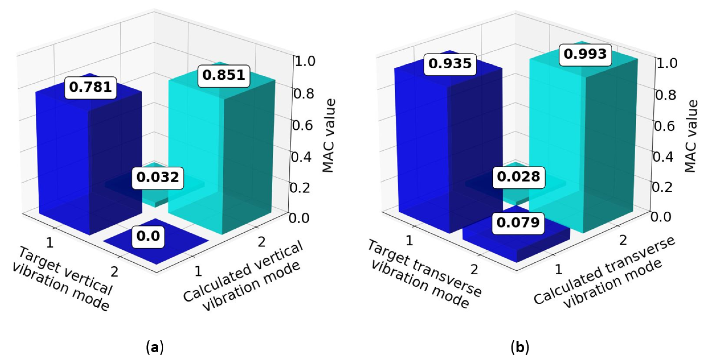
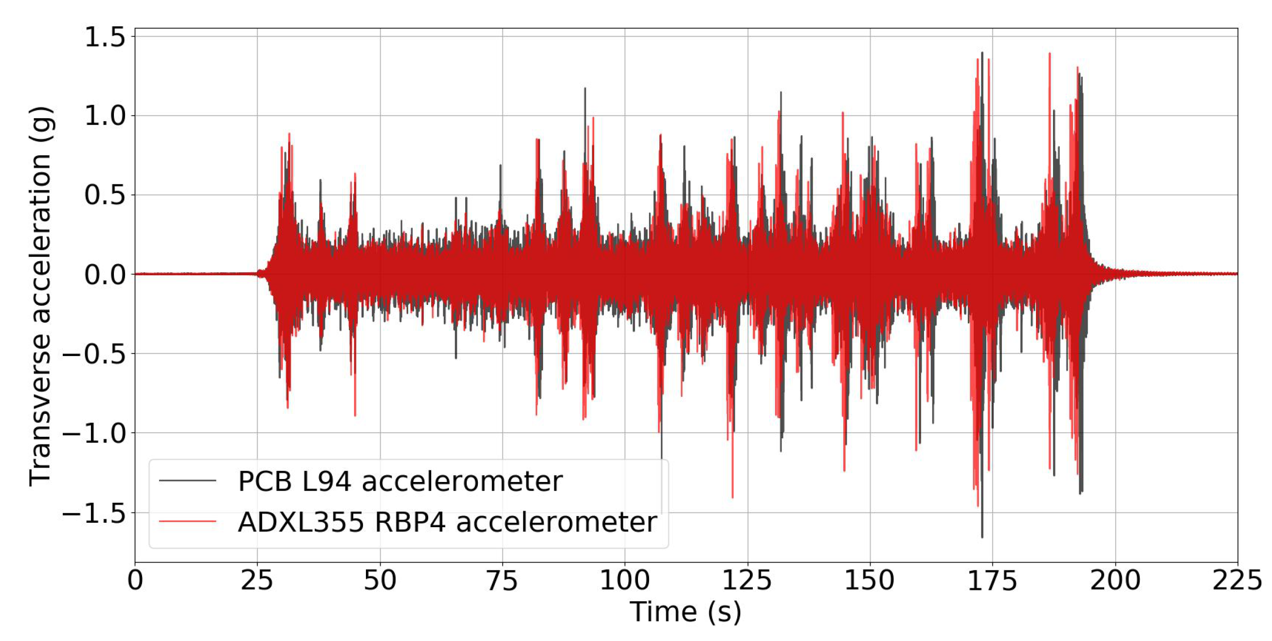
4.2.2. Railway Bridge Monitoring
5. Conclusions
Author Contributions
Funding
Institutional Review Board Statement
Informed Consent Statement
Data Availability Statement
Acknowledgments
Conflicts of Interest
References
- Farrar, C.R.; Worden, K. An introduction to structural health monitoring. Philos. Trans. R. Soc. A Math. Phys. Eng. Sci. 2007, 365, 303–315. [Google Scholar] [CrossRef] [PubMed]
- Yuen, K.V.; Au, S.K.; Beck, J.L. Two-stage structural health monitoring approach for phase I benchmark studies. J. Eng. Mech. 2004, 130, 16–33. [Google Scholar] [CrossRef]
- Chen, H.P.; Ni, Y.Q. Structural Health Monitoring of Large Civil Engineering Structures; Wiley Online Library: Hoboken, NJ, USA, 2018. [Google Scholar]
- Nunez, T.; Boroschek, R.; Larrain, A. Validation of a construction process using a structural health monitoring network. J. Perform. Constr. Facil. 2013, 27, 270–282. [Google Scholar] [CrossRef]
- Rice, J.A.; Spencer, B.F., Jr. Flexible Smart Sensor Framework for Autonomous Full-Scale Structural Health Monitoring; Technical Report; Newmark Structural Engineering Laboratory, University of Illinois at Urbana-Champaign: Urbana, IL, USA, 2009. [Google Scholar]
- Cho, S.; Yun, C.B.; Lynch, J.P.; Zimmerman, A.T.; Spencer, B.F., Jr.; Nagayama, T. Smart wireless sensor technology for structural health monitoring of civil structures. Steel Struct. 2008, 8, 267–275. [Google Scholar]
- Cao, J.; Liu, X. Wireless Sensor Networks for Structural Health Monitoring; Springer: Berlin/Heidelberg, Germany, 2016. [Google Scholar]
- Moreu, F.; Li, X.; Li, S.; Zhang, D. Technical specifications of structural health monitoring for highway bridges: New Chinese structural health monitoring code. Front. Built Environ. 2018, 4, 10. [Google Scholar] [CrossRef] [Green Version]
- Lynch, J.P.; Loh, K.J. A summary review of wireless sensors and sensor networks for structural health monitoring. Shock Vib. Dig. 2006, 38, 91–130. [Google Scholar] [CrossRef] [Green Version]
- Sohn, H.; Farrar, C.R.; Hemez, F.M.; Shunk, D.D.; Stinemates, D.W.; Nadler, B.R.; Czarnecki, J.J. A Review of Structural Health Monitoring Literature: 1996–2001; Los Alamos National Laboratory: Los Alamos, NM, USA, 2003; Volume 1. [Google Scholar]
- Javadinasab Hormozabad, S.; Gutierrez Soto, M.; Adeli, H. Integrating structural control, health monitoring, and energy harvesting for smart cities. Expert Syst. 2021, 38, e12845. [Google Scholar] [CrossRef]
- Melendez, A.; Caballero-Russi, D.; Gutierrez Soto, M.; Giraldo, L.F. Computational models of community resilience. Nat. Hazards 2021, 1–32. [Google Scholar] [CrossRef]
- Hartnagel, B.A.; O’Connor, J.; Yen, W.H.; Clogston, P.; Çelebi, M. Planning and implementation of a seismic monitoring system for the Bill Emerson Memorial Bridge in Cape Girardeau, MO. In Proceedings of the Structures Congress 2006: Structural Engineering and Public Safety, St. Louis, MO, USA, 18–21 May 2006; pp. 1–8. [Google Scholar]
- Ni, Y.; Xia, H.; Ko, J. Structural performance evaluation of Tsing Ma Bridge deck using long-term monitoring data. Mod. Phys. Lett. B 2008, 22, 875–880. [Google Scholar] [CrossRef]
- Jang, S.; Jo, H.; Cho, S.; Mechitov, K.; Rice, J.A.; Sim, S.H.; Jung, H.J.; Yun, C.B.; Spencer, B.F., Jr.; Agha, G. Structural health monitoring of a cable-stayed bridge using smart sensor technology: Deployment and evaluation. Smart Struct. Syst. 2010, 6, 439–459. [Google Scholar] [CrossRef] [Green Version]
- Zonta, D.; Wu, H.; Pozzi, M.; Zanon, P.; Ceriotti, M.; Mottola, L.; Picco, G.P.; Murphy, A.L.; Guna, S.; Corra, M. Wireless sensor networks for permanent health monitoring of historic buildings. Smart Struct. Syst. 2010, 6, 595–618. [Google Scholar] [CrossRef] [Green Version]
- Kim, S.; Pakzad, S.; Culler, D.; Demmel, J.; Fenves, G.; Glaser, S.; Turon, M. Health monitoring of civil infrastructures using wireless sensor networks. In Proceedings of the 6th International Conference on Information Processing in Sensor Networks, Cambridge, MA, USA, 25–27 April 2007; pp. 254–263. [Google Scholar]
- Chopra, A.K. Dynamics of Structures; Pearson Education: London, UK, 2012. [Google Scholar]
- Brincker, R.; Ventura, C.E.; Andersen, P. Damping estimation by frequency domain decomposition. In Proceedings of the IMAC 19: A Conference on Structural Dynamics, Kissimmee, FL, USA, 5–8 February 2001; Society for Experimental Mechanics: Bethel, CT, USA, 2001; pp. 698–703. [Google Scholar]
- Pioldi, F.; Ferrari, R.; Rizzi, E. A refined FDD algorithm for Operational Modal Analysis of buildings under earthquake loading. In Proceedings of the 26th International Conference on Noise and Vibration Engineering, Leuven, Belgium, 15–17 September 2014; Volume 1, pp. 3353–3368. [Google Scholar]
- Brincker, R.; Zhang, L.; Andersen, P. Modal identification from ambient responses using frequency domain decomposition. In Proceedings of the 18th International Modal Analysis Conference (IMAC), San Antonio, TX, USA, 7–10 February 2000. [Google Scholar]
- Pastor, M.; Binda, M.; Harčarik, T. Modal assurance criterion. Procedia Eng. 2012, 48, 543–548. [Google Scholar] [CrossRef]
- Rainieri, C.; Fabbrocino, G. Operational Modal Analysis of Civil Engineering Structures; Springer: Berlin/Heidelberg, Germany, 2014. [Google Scholar]
- Tischer, H.; Thomson, P.; Marulanda, J. Comparación de tres transformadas para distribuciones tiempo-frecuencia por medio de su aplicación a registros de vibraciones ambientales. Ingeniería Compet. 2007, 9, 21–32. [Google Scholar] [CrossRef]
- Raspberry Pi Foundation. Raspberry Pi 3 Model B+; Technical Report; Raspberry Pi Foundation: Cambridge, UK, 2018. [Google Scholar]
- Allied Electronics & Automation. Raspberry Pi RASPBERRY PI 3 MODEL B+. 2020. Available online: https://en-co.alliedelec.com/product/raspberry-pi/raspberry-pi-3-model-b-/71131895/?src=raspberrypi (accessed on 5 August 2020).
- Analog Devices. Data Sheet ADXL354/ADXL355; Technical Report; Analog Devices Inc.: Norwood, MA, USA, 2018. [Google Scholar]
- Analog Devices. EVAL-ADXL35X. 2020. Available online: https://www.analog.com/en/design-center/evaluation-hardware-and-software/evaluation-boards-kits/EVAL-ADXL35X.html#eb-overview (accessed on 14 May 2020).
- ElectronicWings. RASPBERRY PI I2C. 2019. Available online: https://www.electronicwings.com/raspberry-pi/raspberry-pi-i2c (accessed on 19 December 2019).
- Mills, D.L. Internet time synchronization: The network time protocol. IEEE Trans. Commun. 1991, 39, 1482–1493. [Google Scholar] [CrossRef] [Green Version]
- National Instruments. NI 9234 Datasheet; Technical Report; National Instruments Inc.: Austin, TX, USA, 2015. [Google Scholar]
- Quanser. Shake Table II Datasheet; Technical Report; Quanser Inc.: Markham, ON, Canada, 2019. [Google Scholar]
- Hilti. Manual Martillo Rompedor TE 1000-AVR/TE 1500-AVR; Technical Report; Hilti Corporation: Schaan, Liechtenstein, 2013. [Google Scholar]
- Freire Obregón, C. Implementación y Validación del método Mejorado de Descomposición en el Dominio de la Frecuencia (EFDD) para la Identificación de los Parámetros Modales de Estructuras genéricas Utilizando Ruido Ambiente. Estudio del Rango de Aplicabilidad en función del Modelo Estructural y las Condiciones de uso. Master’s Thesis, Universidad de Las Palmas de Gran Canaria, Las Palmas, Spain, 2011. [Google Scholar]
- Magalhães, F.; Cunha, Á.; Caetano, E.; Brincker, R. Damping estimation using free decays and ambient vibration tests. Mech. Syst. Signal Process. 2010, 24, 1274–1290. [Google Scholar] [CrossRef] [Green Version]
- Caballero, D. Caracterización Dinámica de Estructuras Empleando un Sistema de Monitoreo de Salud Estructural de bajo Costo. Master’s Thesis, Universidad del Norte, Barranquilla, Colombia, 2021. [Google Scholar]


| Monitored Structure (Year) | Type of SHM System | Estimated Cost of SHM System (USD) | Estimated Cost per Node (USD) |
|---|---|---|---|
| Tsing Ma Bridge (1997) | Traditional | $8,000,000 | $26,667 |
| Bill Emerson Memorial Bridge (2005) | Traditional | $1,500,000 | $17,857 |
| Golden Gate Bridge (2006) | Wireless network | $38,400 | $600 |
| Aquila Tower (2008) | Wireless network | $1429 | $89 |
| Jindo Bridge (2009) | Wireless v | $35,000 | $500 |
| Feature | Accelerometers | ||
|---|---|---|---|
| Model | 356B18 | 356B18 | 333B50 |
| Measurement axes | Triaxial | Triaxial | Uniaxial |
| Reference name | PCB L94 | PCB L74 | PCB L12 |
| Sensitivity (mV/g) | 1000 | 1000 | 1000 |
| Measurement range (V) | ±5.0 | ±5.0 | ±5.0 |
| Frequency range ±5.0% (Hz) | 0.5–3000 | 0.5–3000 | 0.5–3000 |
| Cost (USD) | $1764 | $1764 | $598.5 |
| Acceleration Spectrum | Accelerometer | Accelerations Range (g) | R2 | RMS Error (g) |
|---|---|---|---|---|
| Original sampling frequency | PCB L74 | 0.10–0.21 | 0.784 | - |
| ADXL355 RBP1 | 0.11–0.20 | 0.848 | 0.010 | |
| ADXL355 RBP4 | 0.088–0.21 | 0.873 | 0.012 | |
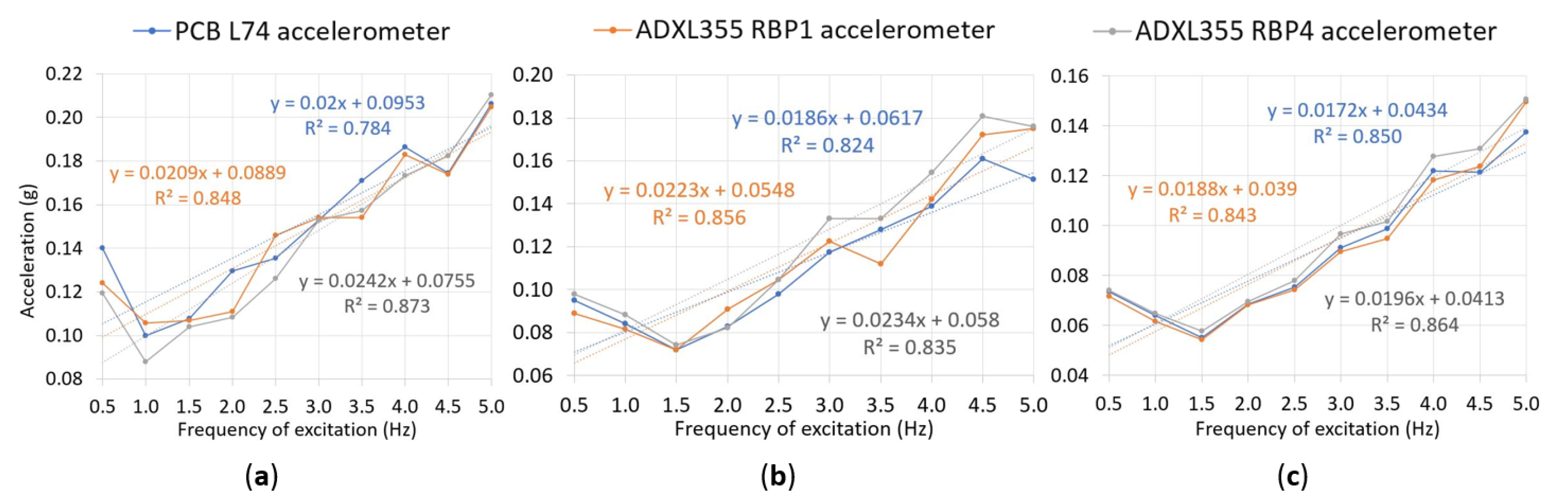
| 100 Hz resampling frequency | PCB L74 | 0.072–0.16 | 0.824 | - |
| ADXL355 RBP1 | 0.072–0.18 | 0.856 | 0.011 | |
| ADXL355 RBP4 | 0.074–0.18 | 0.835 | 0.013 | |
| Highest 100 acceleration peaks mean | PCB L74 | 0.055–0.14 | 0.850 | - |
| ADXL355 RBP1 | 0.054–0.15 | 0.843 | 0.0043 | |
| ADXL355 RBP4 | 0.058–0.15 | 0.835 | 0.0059 |
| Acceleration Spectrum | Accelerometer | Accelerations Range (g) | R2 | RMS Error (g) |
|---|---|---|---|---|
| Original sampling frequency | PCB L74 | 0.11–0.47 | 0.940 | - |
| ADXL355 RBP1 | 0.10–0.44 | 0.975 | 0.020 | |
| ADXL355 RBP4 | 0.11–0.49 | 0.917 | 0.030 | |
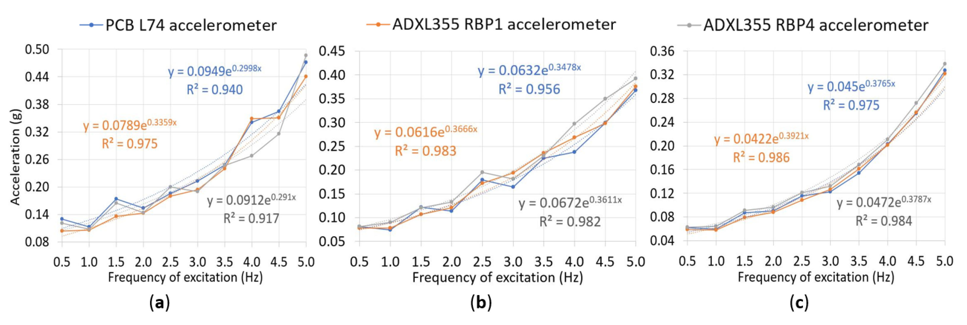
| 100 Hz resampling frequency | PCB L74 | 0.074–0.37 | 0.956 | - |
| ADXL355 RBP1 | 0.078–0.38 | 0.983 | 0.015 | |
| ADXL355 RBP4 | 0.081–0.39 | 0.982 | 0.028 | |
| Highest 100 acceleration peaks mean | PCB L74 | 0.059–0.33 | 0.975 | - |
| ADXL355 RBP1 | 0.058–0.32 | 0.986 | 0.0049 | |
| ADXL355 RBP4 | 0.063–0.34 | 0.984 | 0.0093 |
| Acceleration Spectrum | Accelerometer | Accelerations Range (g) | R2 | RMS Error (g) |
|---|---|---|---|---|
| Original sampling frequency | PCB L74 | 0.11–1.08 | 0.987 | - |
| ADXL355 RBP1 | 0.098–0.93 | 0.991 | 0.11 | |
| ADXL355 RBP4 | 0.10–0.98 | 0.991 | 0.090 | |
| 100 Hz resampling frequency | PCB L74 | 0.076–0.81 | 0.990 | - |
| ADXL355 RBP1 | 0.075–0.79 | 0.992 | 0.016 | |
| ADXL355 RBP4 | 0.077–0.80 | 0.990 | 0.032 | |
| Highest 100 acceleration peaks mean | PCB L74 | 0.054–0.68 | 0.993 | - |
| ADXL355 RBP1 | 0.052–0.68 | 0.998 | 0.0077 | |
| ADXL355 RBP4 | 0.056–0.69 | 0.997 | 0.017 |
| Acceleration Spectrum | Accelerometer | Accelerations Range (g) | R2 | RMS Error (g) |
|---|---|---|---|---|
| Original sampling frequency | PCB L74 | 0.19–2.1 | 0.990 | - |
| ADXL355 RBP1 | 0.13–1.33 | 0.976 | 0.28 | |
| ADXL355 RBP4 | 0.15–1.36 | 0.988 | 0.27 | |
| 100 Hz resampling frequency | PCB L74 | 0.11–1.01 | 0.984 | - |
| ADXL355 RBP1 | 0.10–1.04 | 0.988 | 0.015 | |
| ADXL355 RBP4 | 0.11–1.02 | 0.987 | 0.019 | |
| Highest 100 acceleration peaks mean | PCB L74 | 0.071–0.87 | 0.981 | - |
| ADXL355 RBP1 | 0.068–0.89 | 0.985 | 0.0091 | |
| ADXL355 RBP4 | 0.076–0.87 | 0.983 | 0.016 |
| Vibration Mode 1 | |||||
|---|---|---|---|---|---|
| Channel | Frequency (Hz) | Modal Coordinate | |||
| Reference System | Low-Cost System | Reference System | Low-Cost System | ||
| 1 | 1.95 | 1.95 | 0.588 | 0.445 | |
| 2 | 1.000 | 1.000 | |||
| Vibration Mode 2 | |||||
| Channel | Frequency (Hz) | Modal Coordinate | |||
| Reference System | Low-Cost System | Reference System | Low-Cost System | ||
| 1 | 7.81 | 7.81 | 1.000 | 1.000 | |
| 2 | −0.759 | −0.536 | |||
| Vibration Mode 1 | ||||
|---|---|---|---|---|
| Reference System | Low-Cost System | |||
| Mean Damping Ratio (%) | Coefficient of Variation (%) | Mean Damping Ratio (%) | Coefficient of Variation (%) | |
| 2.022 | 46.8 | 2.339 | 36.8 | |
| Vertical Vibration Mode 1 | |||||
|---|---|---|---|---|---|
| Channel | Frequency (Hz) | Modal Coordinate | |||
| Reference System | Low-Cost System | Reference System | Low-Cost System | ||
| 1 | 6.83 | 6.83 | 0.751 | 0.379 | |
| 2 | 1.000 | 1.000 | |||
| 3 | 0.660 | 0.084 | |||
| Vertical Vibration Mode 2 | |||||
| Channel | Frequency (Hz) | Modal Coordinate | |||
| Reference System | Low-Cost System | Reference System | Low-Cost System | ||
| 1 | 15.62 | 15.62 | −0.963 | −0.476 | |
| 2 | 0.301 | −0.022 | |||
| 3 | 1.000 | 1.000 | |||
| Transverse Vibration Mode 1 | |||||
|---|---|---|---|---|---|
| Channel | Frequency (Hz) | Modal Coordinate | |||
| Reference System | Low-Cost System | Reference System | Low-Cost System | ||
| 1 | 2.93 | 2.93 | 0.644 | 0.602 | |
| 2 | 1.000 | 0.882 | |||
| 3 | 0.644 | 1.000 | |||
| Transverse Vibration Mode 2 | |||||
| Channel | Frequency (Hz) | Modal Coordinate | |||
| Reference System | Low-Cost System | Reference System | Low-Cost System | ||
| 1 | 13.67 | 13.67 | −1.000 | −0.844 | |
| 2 | 0.216 | 0.201 | |||
| 3 | 1.000 | 1.000 | |||
| Vertical Vibration Mode 1 | ||||
|---|---|---|---|---|
| Reference System | Low-Cost System | |||
| Mean Damping Ratio (%) | Coefficient of Variation (%) | Mean Damping ratio (%) | Coefficient of Variation (%) | |
| 3.54 | 19.2 | 3.63 | 22.8 | |
| Transverse Vibration Mode 1 | ||||
| Reference System | Low-cost System | |||
| Mean Damping Ratio (%) | Coefficient of Variation (%) | Mean Damping ratio (%) | Coefficient of Variation (%) | |
| 1.553 | 21.1 | 1.514 | 24.4 | |
Publisher’s Note: MDPI stays neutral with regard to jurisdictional claims in published maps and institutional affiliations. |
© 2022 by the authors. Licensee MDPI, Basel, Switzerland. This article is an open access article distributed under the terms and conditions of the Creative Commons Attribution (CC BY) license (https://creativecommons.org/licenses/by/4.0/).
Share and Cite
Caballero-Russi, D.; Ortiz, A.R.; Guzmán, A.; Canchila, C. Design and Validation of a Low-Cost Structural Health Monitoring System for Dynamic Characterization of Structures. Appl. Sci. 2022, 12, 2807. https://doi.org/10.3390/app12062807
Caballero-Russi D, Ortiz AR, Guzmán A, Canchila C. Design and Validation of a Low-Cost Structural Health Monitoring System for Dynamic Characterization of Structures. Applied Sciences. 2022; 12(6):2807. https://doi.org/10.3390/app12062807
Chicago/Turabian StyleCaballero-Russi, David, Albert R. Ortiz, Andrés Guzmán, and Carlos Canchila. 2022. "Design and Validation of a Low-Cost Structural Health Monitoring System for Dynamic Characterization of Structures" Applied Sciences 12, no. 6: 2807. https://doi.org/10.3390/app12062807
APA StyleCaballero-Russi, D., Ortiz, A. R., Guzmán, A., & Canchila, C. (2022). Design and Validation of a Low-Cost Structural Health Monitoring System for Dynamic Characterization of Structures. Applied Sciences, 12(6), 2807. https://doi.org/10.3390/app12062807