Acoustic Emission Based Fault Detection of Substation Power Transformer

Abstract

Fault detection of Substation Power Transformer by Non-contact measurement is important for the safety of machines, instruments, and human beings. To make non-contact measurement as convenient as possible, it is desirable that efficient algorithms based on AE (acoustic emission) discrimination are developed. This paper presents a system for quick and effective fault detection of substation power transformer, based on AE signals collected by non-contact single microphones. In the experiment, collected data were preprocessed in multiple ways and three machine learning algorithms were designed based on classifiers (Convolutional Neural Network (CNN), support vector machine (SVM), and k-nearest neighbors (KNN) algorithm) trained and tested by a tenfold cross-validation technique. After comparison among the designed classifiers, the results show the two-dimensional principal component analysis (2DPCA) preprocess combined with SVM achieved the best comprehensive effectiveness.

1. Introduction

Non-contact measurement [1,2], nondestructive testing [3,4,5,6,7] are the key components of robot automatic inspection technology, especially faced with some dangerous, precious, or tender tested objects. Usually, based on some special sensors designed according to one or several physics theories, some features related to the inspected devices were extracted from the recorded signals, then using these features the computer system undertakes the analysis and diagnose work. Up to now, many systems in which the non-contact measurement or nondestructive measurement were applied have already been deployed to the market and have played useful roles in everyday life. For example, the system for detecting ferromagnetic plates using electromagnetic acoustic lamb waves [8], velocity measurement of moving objects by non-contact Doppler radar [9], and machine vision techniques [10], etc. Although many important results of non-contact measurement have already been reported and many systems have already been applied in the field, the technologies and theories are still far from being mature. There are many problems still waiting for solutions, i.e., the high complexity of the device makes it difficult to operate, and the physics parameters conveying useful information used for testing are hardly generated. Comparatively speaking, acoustic signals, as a most essential tool for human communication, is a simpler manner of non-contact measurement than other manners such as optical, electricity, and magnetism in non-contact measurement. A successful application of AE signals in the field of non-contact measurement can not only improve security but also decrease the occupation of resources [8,11,12].

Automatic fault detection of power transformers by AE signals is a typical application of non-contact measurement. Different running states of the equipment can emit different AE signals with different spectra information. These spectra information can be used as the features of different running states of the equipment. Experienced engineers can discriminate the operational status of the transformer according to the AE signals. This is mainly based on the Human ear perception for spectral information. Especially in the power system, it has been relying on manual detection for a long time, which is low efficiency, non-real-time, and lack of security. Early fault detection of power transformer often involves routine inspections, preventive testing, and insulation oil test, which are mainly based on the traditional human participation, and this working mode for inspections has played a crucial role for safe and stable operation of substation. With the continuous expansion of the scale of the power system, the complexity of equipment, and the application of high technology, this mode cannot keep up with the need for inspection. At this point, automatic fault detection by acoustic signals utilizing its safety and convenience has been considered to meet the demand of the scale of a constantly complex system.

Currently machine learning methods are more and more used in transformer fault identification. Most of the research and experiments are carried out in many cases. Due to the rapid development of speech recognition and the similarity between other kinds of AE signals and speech, many ideas of AE based event detection [13,14] and device running monitoring [15] come from automatic speech recognition (ASR) [16], and the input feature is similar with speech (such as short-time power spectrum, short-time zero-crossing rate, short-time autocorrelation function, etc.). These algorithms used to distinguish events are relatively traditional machine learning algorithms such as k-nearest neighbor and decision tree. In recent years, with the significant improvement of computer computing speed and storage, machine learning under big data has become a research hotspot. As a branch of machine learning, Deep learning [17] imitates the human brain to model patterns in data as complex multi-layer networks. At present, deep learning has also been widely applied in AE fault-based detection [18,19].

Although the rapid developing of deep learning has boomed, the traditional methods still retain some advantages in some aspects. While deep learning needs the support of large amount of data, the traditional methods are more suitable to small data process. In many cases, the data of different running status are severe imbalance. As a result, the trained model is easy to be trapped overfitting. In addition, the issue of efficiency and resource saving is also difficulty posted in front of system designers. Some of the traditional methods need not consume a lot of training resources, so that they can easily realize incremental improvement of the parameters in the models. Others may have good generalization suitable for small data training. Different classifier has different character, how to select a suitable classifier is also an important issue for the designer.

In this study, we compare the effectiveness of several common classifiers on transformer sound classification. The results can be a reference for the transformer faults detection system design. We also discussed the PCA (principal component analysis) [20] method, the 2DPCA [21] (two-dimensional principal component analysis) method and their feature dimension selection, and presented the CNN (convolutional neural network) [22] method, as a compared method in the results tables. We divided the issues into the two-category problem, in which normal emission signals with various noises are regarded as normal emission signals, and multi-classification problem, in which normal sound and normal sound with various noises are regarded as different patterns.

This paper unfolds in the following fashion. Section 2 presents the dataset for transformer sound classification assessment, including the data acquisition, data preprocessing and labeling. Section 3 demonstrates the detailed of the different classifier models, feature process and evaluation Criteria. Section 4 takes the two two-category problem and multi-classification problem as the examples to show the efficiency of the several models. Section 5 gives the discussion for the results and some questions and final conclusions are illustrated in Section 6.

2. Dataset

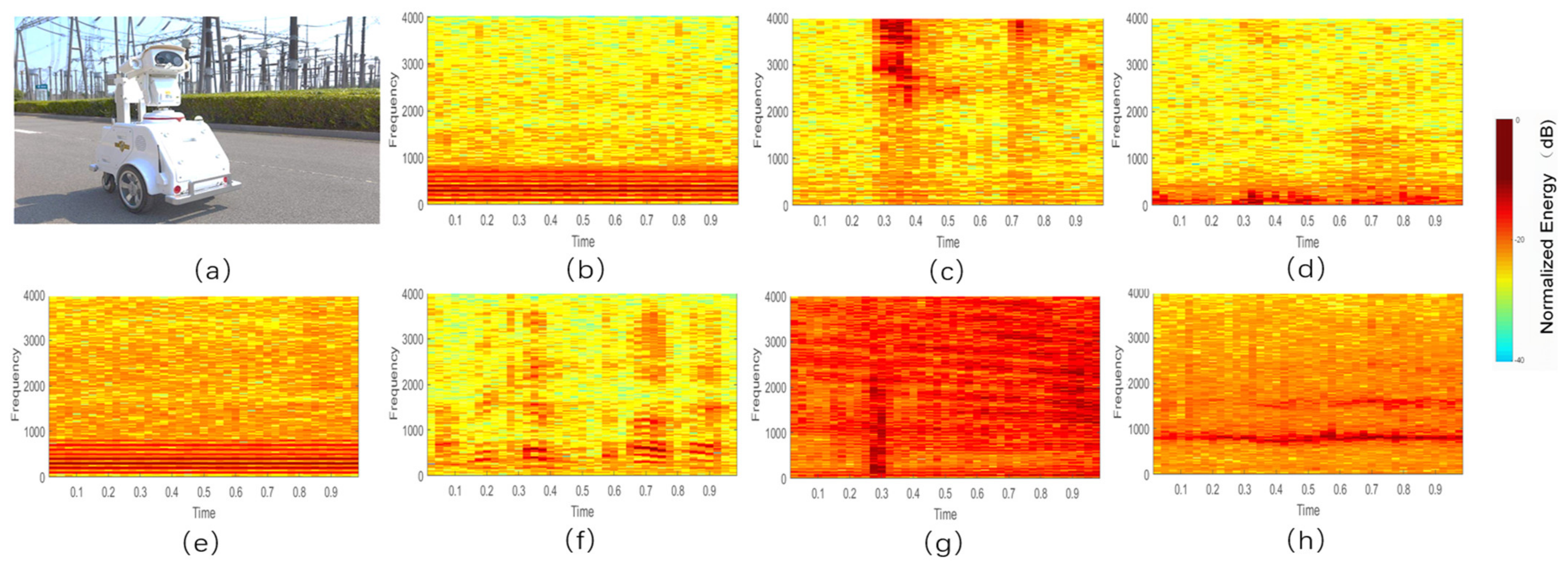
The samples of AE signals were collected from 36 transformers located in six transformer stations. The length of each segment of AE signals is about 10 min. To ensure uniformity of all collected AE signals samples, the same sampling equipment is used for each acquisition, and the sampling rate is fixed. The acquisition equipment includes a pickup connected with the Intel NUC5i7RYB PC fixed in an acoustic and vision inspection robot (Figure 1a). The original sampling rate is set at 22,050 Hz, and then the output signals were downsampled to 16 k/s and encoded to 16-bit format with a single-channel configuration. The measurements were made in real time and all data were obtained in natural scenarios. For analyzing these data, every 10 min of data is linear normalized as follows.

Y = (2 × (X − X_min))/(X_max − X_min) − 1

(1)

where X is the original AE signals data, X_min represents the minimum amplitude in the AE signals data, X_max represents the maximum amplitude in the AE signals data, and Y is the data after normalization.

As the AE signals of the transformer is basically long time stationary, in the following processing step, the level-adjusted signal is subdivided into overlapping fragments of 1.0 s duration (16 K samples) with an overlap of 0.5 s, which are classed and labeled with normal clean, normal with bird call, normal with wind, normal with rain and normal with the human voice, discharge and mechanical sliding signals.

Figure 1 also illustrates the spectrogram of the seven kinds of acoustic patterns. It can be seen from the spectrograms, apart from the normal signals with bird call bird call and human voice, other patterns are time-stationary. Whether with noises or not, there are obvious visual differences between the normal signals Figure 1b–f and the fault signals Figure 1g,h. However, within the normal signals b, d and e, the difference is not notable, strictly to say, they are all the normal signal in practice and need not to be distinguished, in this paper, we make the discrimination for them just for test the performance of different classification methods. The difference between the two fault signals Figure 1g,h is bigger than the normal signals. The normalized energy in the spectrogram of discharge signals is more concentrated in the low frequency region, and in high frequency region, the transient energy concentration can be seen randomly.

Therefore, when we are extracting the feature of the signals, we don’t think the sound of wind, rain, birds singing and human voice as noises and carry suppression and removal operation.

After selection (deleting some blank and invalid data), the total number of the sound fragments of 1.0 s duration used in the following experiments is 15,520, and tenfold cross validation was used for testing the reliability of the classification system, in each test the training set includes 90% of total samples, and 10% of total samples used as the test samples. The specific description as shown in

Table 1. Sample distribution in the seven different types of AE signals and division of normal and fault samples in binary classification.

AE Signals Type	Normal					Fault
	Normal Clean (A)	Normal with Bird Call (B)	Normal with Wind (C)	Normal with Rain (D)	Normal with Voice (E)	Discharge Signals (F)	Mechanical Signals (G)
Total samples	4000	1200	4000	4000	2000	160	160
Testing samples	400	120	400	400	200	16	16

. We can see that the number of samples for different classes is seriously unbalanced which leads to over fitting of the solution and lack of generalization ability.

3. Methods

3.1. Feature Extraction

Joint time-frequency representation is the most common technique used in the AE signals signal process. The effective signals are transferred into a time-frequency representation to yield [23]:

$$X_n\left(e^{j\omega }\right)={{\displaystyle \sum }}_{m=-\infty }^{\infty }x\left(m\right)\omega \left(n-m\right)e^{-j\omega m}$$

(2)

where x(n) is the signal received after endpoint detection and ω(n) is the window function, which shifts the AE signals signal by one step length on the time axis. As one of the joint time-frequency representations, the spectrogram, has demonstrated its good prospects for the information in the signals. The spectrogram representation X can be calculated as,

$$X=|X_n\left(e^{j\omega }\right){|}^2$$

(3)

For acquiring the spectrogram of each segment, the 1.0 s segment is subdivided into overlapping sub-segments of 50 ms duration (800 samples) with a progression of 25 ms (400 samples). Each sub-segment is multiplied with a hamming window and padded with zeros to obtain a frame of 1024 samples. After doing so, we can obtain a 512 × 39 spectrogram of the 1-s signal as shown in Figure 1. Figure 1 also demonstrates that the energy of the AE signals is mainly concentrated in the low-frequency region, whether in the normal state or the discharging state, and the distribution of the energy becomes sparse with the increase of the frequency. Due to uneven resolution of the human auditory system to frequency domain [24], for example, the human ear is more sensitive to low frequency, Mel-scale is often used in the speech and audio process. Although there is a well-defined Mel-scale frequency band division formula, we find that the division effect will be better after properly adjust. Here the frequency band is divided into 8 sub-bands (1~60, 61~125, 126~180, 181~240, 241~300, 301~365, 366~425, 426~512). Considering the entire difference of different patterns, the energy of the sub-segment calculated as an energy term was appended to form a feature vector with nine feature parameters for each sub-segment. Therefore, every one-second segment has a total of 9 × 39 feature vectors such as Figure 2. Compared with Figure 1, the differences of the spectrograms between the normal operating state (Figure 2a) and the discharged state (Figure 2b) become more evident. Furthermore, the burr that appears in the spectrogram (Figure 1b) is also significantly attenuated in the 9 × 39 feature vector (Figure 2b).

3.2. Feature Dimension Reduction

Although the sub-band energies characteristic parameters can well reflect the AE signals features and have smaller sizes than the speech samples, many redundancies are still exited in the feature representations. Usually, the redundancies can reduce the classification sensitivity, and consume more resources of the calculation. PCA as a linear transform of data has good performance in redundancies reduction, and it can supply a good choice for us to test if the reduction of data increases the classification sensitivity. The PCA method is also called the one-dimensional principal component analysis, that is to say, the data object to reduce dimensionality is a one-dimensional vector form composed of many features. While 2DPCA is also a dimensionality reduction method that is directly applied to the two-dimensional feature matrix. Compared with the PCA method, the 2DPCA method is more efficient and has less computation in calculating the covariance matrix, so it has greater advantages in imaging progress. In this paper, the PCA and the 2DPCA methods were considered and their effects in SVM and kNN [25] were investigated.

3.2.1. For Analysis with PCA

Firstly, the two-dimensional spectrogram feature of 1 s AE signals data was transferred to a one-dimensional vector via a one-by-one connection of the column vector. After the treatment, each vector of the 1 s AE signals is composed of 9 × 39 characteristic parameters. The central calculation of the PCA method is to find the covariance matrix for the new one-dimensional vector, and then find the eigenvalues of the covariance matrix and its corresponding eigenvectors, and finally find the optimal projection axis. For choosing the optimal projection axis, we set the eigenvalue contribution reconstruction threshold μ according to the research needs. The eigenvalue contribution reconstruction threshold μ is between 0 and 1. After the eigenvalues ${\lambda }_i$ are sorted from large to small, the eigenvalue contribution is calculated as follows:

$$\mu =\frac{{{\displaystyle \sum }}_{i=1}^k{\lambda }_i}{{{\displaystyle \sum }}_{i=1}^n{\lambda }_i}\hspace{1em}\hspace{1em}\hspace{1em}\hspace{1em}\hspace{1em}1\le k\le n$$

(4)

In general, the larger the eigenvalue contribution is the more information about the original data we keep. The PCA method used in this paper mainly includes the following steps:

Constructing total sample matrix: We employ a total of 13,968 (90% of total samples) samples as training data, which take the feature row vectors of each AE signals data of the training sample as a row of the two-dimensional matrix into a 171 × 13,968 matrix.

Standardizing the total sample matrix: the mean of each row of the training sample matrix is obtained and the mean of the corresponding row is subtracted from each feature value in the row to obtain a new two-dimensional feature matrix. In the testing process, the feature vectors of the test sample also need the standardizing process a,

$$x_{ij}{}^{*}=x_{ij}-\overline{x_{ij}}$$

(5)

where $\overline{x_{ij}}=\frac{1}{n}{{\displaystyle \sum }}_{i=1}^n{x}_{ij}$. The covariance matrix of the new feature matrix of the training sample is calculated. The eigenvalues and eigenvectors of the covariance matrix are calculated and the eigenvalues are arranged in descending order. The eigenvalue contribution will be calculated and discussed in the results and discussion section of this paper. By selecting the different eigenvector sequence length according to the order from large to small, the different projection matrix of the optimal projection axis is obtained and can be used for dimension reduction and performance comparison.

After the standardization process, the feature of each 1 s data (training sample, test sample) is projected onto the projection matrix, and the new feature of the training sample and the testing sample is obtained which can achieve different dimension reduction effects by selected different eigenvector sequence length.

3.2.2. For Analysis with 2DPCA

Compared with PCA, 2DPCA is based on 2D matrices rather than 1D vectors, which means the covariance matrix can be constructed directly by the original matrices. According to the definition of 2DPCA, we can calculate the eigenvalue and orthonormal eigenvectors from feature extraction. This virtually reduces the amount of calculation. On the other hand, compared with the PCA method, the covariance matrix constructed by 2DPCA is smaller, so it takes less time to acquire eigenvectors. Similar to Equation (4) in the PCA method, by selecting the number of feature eigenvalue and the corresponding eigenvector in accordance with the order from big to small, the optimal projection vectors of 2DPCA can be calculated. At last, for every spectrogram representation, we can acquire the dimension reduction representations of the samples.

3.3. Machine Learning Algorithms

3.3.1. Support Vector Machine

Support Vector Machine (SVM) is to project nonlinear inseparable samples into high-dimensional space by taking advantage of the kernel functions and then locate the optimal separating hyperplane in the projection space by solving a quadratic optimization problem. Typical kernel functions of SVM including the following four kinds:

• Linear kernel functions [26]: $k\left(x_i,x_j\right)=\langle x_i,x_j\rangle +c$
• Radial basis functions (RBF) [27]: $k\left(x_i,x_j\right)=exp\left[-\frac{1}{2{\sigma }^2}\left|\right|x_i-x_j\left|\right|\right]$
• Sigmoidal kernel functions: $k\left(x_i,x_j\right)=tanh\left(k\langle x_i,x_j\rangle +c\right)$
• Polynomial kernel functions: $k\left(x_i,x_j\right)={\left({\rm Y}\langle x_i,x_j\rangle +\gamma \right)}^d$

In this paper, we use the above four kernel functions in the following experiment. In addition, from the results of classification, we compared the performances of the four optimized kernel functions with each other.

3.3.2. kNN

k-nearest neighbor (kNN)—A nonparametric method used for classification and regression [28]. kNN is a classical and relatively simple classifier. It classifies an unknown sample x by assigning it the label most frequently represented among the k nearest samples, which means a decision can be made by taking a vote for the labeled k nearest neighbors.

Usually only two parameters are needed in this method, they are Number of neighbors and Distance metric. In this work, we selected these parameters as follows:

• Number of neighbors: k = 5
• Distance metric: Minkowski
• The input of the kNN model is the 9 × 39 feature vectors (Figure 2).

3.3.3. CNN

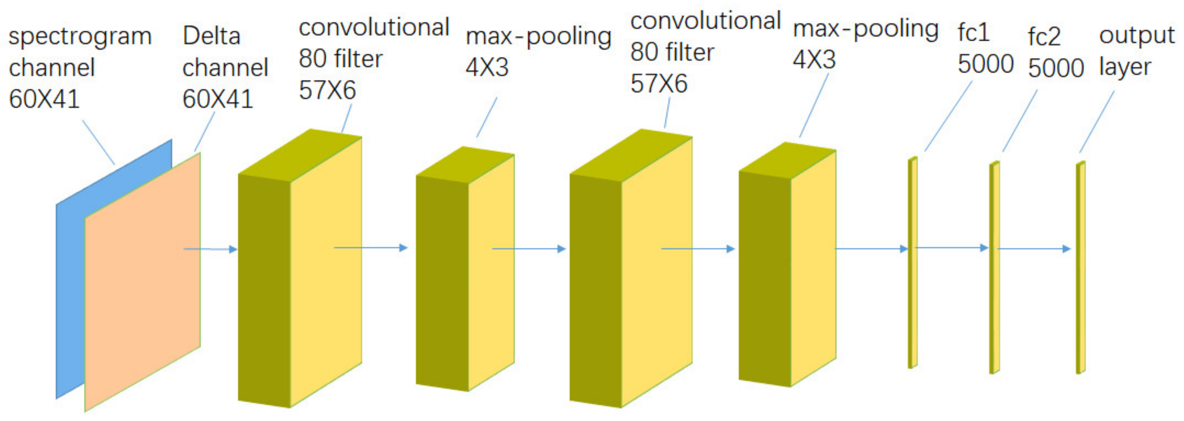
The CNN model used as a comparison is referenced from Piczak’s work [29]. First, the recording data in Table 1 were resampled to 22,050 Hz and normalized, then Log-scaled Mel-spectrograms were extracted with a window size of 1024, hop length of 512, and 60 mel-bands, using the librosa [30] implementation. At last, Segments (e.g., 60 rows/bands × 41 columns/frames) were provided together with their deltas (computed with default librosa settings) as a 2-channel input to the network.

The detailed network architecture of CNN in this work is rewrite as Figure 3.

3.4. Evaluation Criteria

The fault discrimination problem described in this paper belongs to a typical binary classification problem, and sensitivity is an important evaluation index. However, due to the extremely uneven number of samples in positive and negative categories, simply using sensitivity as an indicator cannot well quantify performance of a classifier. In fact, In the binary classification problem, we should investigate the positive (fault sample) and negative (normal samples) categories at same time. Therefore, the accuracy rates are also discussed in our binary classification experiments.

Sensitivity (SEN), and accuracy in the binary classification were calculated as averages over the 10 cross-validation cases according to the following formulas:

SEN = TP/P

(6)

Accuracy = (TP + TN)/(TP + TN + FP + FN)

(7)

Where True positives (TP), true negatives (TN), false positives (FP), and false negatives (FN), are the four different possible outcomes of a single prediction for a two-class case with classes “1” (“yes”) and “0” (“no”). A false positive is when the outcome is incorrectly classified as “yes” (or “positive”), when it is in fact “no” (or “negative”). A false negative is when the outcome is incorrectly classified as negative when it is in fact positive. True positives and true negatives are obviously correct classifications.

For estimating the overall performance in multi-classification problems, the average SEN of multi-class was used and it can be defined as

$$\begin{array}{c}\mathrm{SEN}=\frac{{{\displaystyle \sum }}_{n=1}^{N}CR/\left(CR+IU\right)}{N}\end{array}$$

(8)

where

(1)

N—Number of sets for cross validation;

(2)

IU—Incorrectly unrecognized = number of erroneous classifications (which is equal to the sum of the off diagonal entries of the confusion matrix);

(3)

CR—Correctly recognized = (number of elements in the test set number of classes) − number of erroneous classifications.

In addition to the sensitivity index, kappa [31] coefficient is also used as the performance evaluation parameter in the muti-classification experiments.

In this study, the computations were run on an Intel Core i7-6700 3.4 GHz, 32-GB RAM machine. For different classifier and different parameters, there is a big difference in training time. For the CNN, the GPU was used in the training process. Compared with training, test time is more related to actual application. Based on this, we only count the time spent in the test phase. SVM program used in the simulation process is LIBSVM designed by Professor Lin Zhiren [28] of Taiwan University.

4. Results and Discussions

4.1. Relationship between Reconstruction Threshold and the Number of Eigenvectors in PCA and 2DPCA

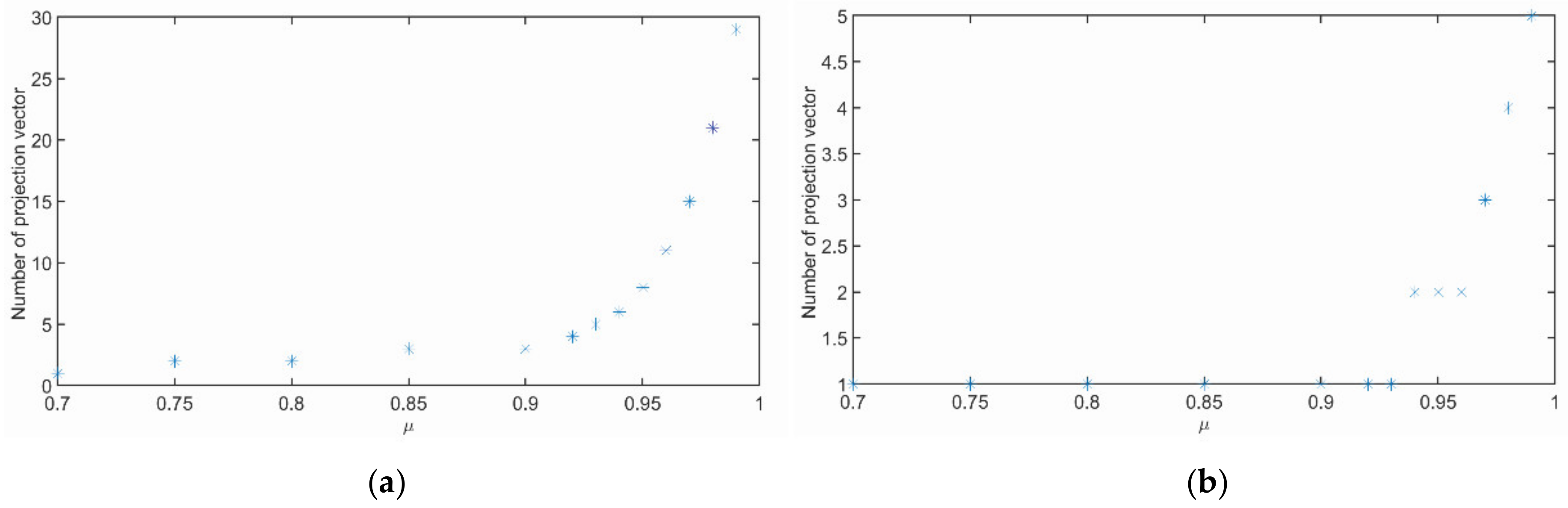
In PCA analysis (Figure 4a), the first two coefficients account for a larger proportion, while In 2DPCA analysis (Figure 4b), the first coefficient account for a larger proportion, With the $\mu$ increase, the number of eigenvectors 2DPCA analysis change more slowly.

4.2. The Fault Detection by SVM Binary Classification Method

When the dimensionality reduction reconstruction threshold is set to 0.75, the effect of different kernel functions on the fault detection accuracy is shown in

Table 2. Results of the experiment for testing sets including three machine learning algorithms, tenfold cross validation, and six variants of signal preprocessing results of the binary classification experiment.

Algorithms		Preprocessing
		Without PCA	With PCA (Sum = 1552, 1520, 32)			With 2DPCA (Sum = 1552, 1520, 32)
			μ = 0.75 Projection = 2	μ = 0.9 Projection = 3	μ = 0.96 Projection = 10	μ = 0.75 Projection = 1	μ = 0.95 Projection = 2	μ = 0.99 Projection = 5
SVM	Linear	ERR sum = 1043 ACC = 93.28% SEN = 84.69% test time = 11.28 s	ERR sum = 18 ACC = 99.88% SEN = 97.5% test time = 2.520 × 10 −2 s	ERR sum = 29 ACC = 99.81% SEN = 96.25% test time = 4.033 × 10−2 s	ERR sum = 171 ACC = 98.90% SEN = 91.56% test time = 1.210 s	ERR sum = 6 ACC = 99.96% SEN = 100% test time = 0.568 s	ERR sum = 98 ACC = 99.37% SEN = 100% test time = 0.996 s	ERR sum = 1667 ACC = 89.26% SEN = 96.87% test time = 2.397 s
	RBF	ERR sum = 3235 ACC = 79.16% SEN = 53.25% test time = 15.11 s	ERR sum = 2030 ACC = 86.92% SEN = 85.32% test time = 2.970 × 10 −2 s	ERR sum = 2991 ACC = 80.73% SEN = 84.06% test time = 3.021 × 10−2 s	ERR sum = 3026 ACC = 80.50% SEN = 83.44% test time = 0.550 s	ERR sum = 2032 ACC = 86.87% SEN = 91.25% test time = 0.880 s	ERR sum = 2038 ACC = 86.86% SEN = 90.31% test time = 1.362 s	ERR sum = 2047 ACC = 86.81% SEN = 89.37% test time = 4.110 s
	Sigmoidal	ERR sum = 2876 ACC = 81.47% SEN = 72.19% test time = 11.22 s	ERR sum = 2172 ACC = 86.01% SEN = 100% test time = 2.017 × 10−2 s	ERR sum = 2047 ACC = 86.81% SEN = 98.87% test time = 2.460 × 10−2 s	ERR sum = 2100 ACC = 86.47% SEN = 97.5% test time = 0.345 s	ERR sum = 101 ACC = 99.35% SEN = 100% test time = 0.820 s	ERR sum = 1860 ACC = 88.02% SEN = 95.31% test time = 1.028 s	ERR sum = 1970 ACC = 87.31% SEN = 90% test time = 3.980 s
	Polynomial	ERR sum = 4061 ACC = 73.83% SEN = 87.81% test time = 13.10 s	ERR sum = 2628 ACC = 83.07% SEN = 93.44% test time = 2.861 × 10−2 s	ERR sum = 2719 ACC = 82.48% SEN = 87.81% test time = 6.387 × 10−2 s	ERR sum = 3633 ACC = 76.59% SEN = 68.13% test time = 0.794 s	ERR sum = 1380 ACC = 91.11% SEN = 96.88% test time = 2.350 s	ERR sum = 2527 ACC = 83.72% SEN = 83.44% test time = 4.061 s	ERR sum = 3515 ACC = 77.35% SEN = 49.06% test time = 11.265 s
KNN	k = 5 p = 2	ERR sum = 988 ACC = 93.63% SEN = 94.06% test time = 13.58 s	ERR sum = 314 ACC = 97.98% SEN = 91.25% test time = 2.907 × 10−1 s	ERR sum = 1314 ACC = 91.53% SEN = 91.25% test time = 6.125 × 10−1 s	ERR sum = 1515 ACC = 90.24% SEN = 94.69% test time = 1.301 s	ERR sum = 1121 ACC = 92.78% SEN = 94.69% test time = 2.205 s	ERR sum = 2334 ACC = 92.78% SEN = 94.69% test time = 4.387 s	ERR sum = 2511 ACC = 83.82% SEN = 87.18% test time = 10.390 s
CNN		ERR sum = 2766 ACC = 82.18% SEN = 91.88% test time = 6.060 s

. In this case, the PCA projection matrix is the size of 171 × 2, the feature vector dimension of each frame is reduced to 2; 2DPCA projection matrix is 9 × 1 vector, the feature matrix is reduced from 39 × 9 to a 39 × 1 vector.

Sliding AE signals and discharge AE signals are taken as fault samples, they constitute the fault category, the others constitute the normal category (see Table 1). From Table 2, the application of different kernel functions has an evident influence on the performance SVM. In the application of linear kernel function [25], the fault detection accuracy rate of both PCA and 2DPCA combined with SVM reach 100%. However, the detection results obtained by the 2DPCA + SVM are better than those of PCA + SVM in the application of other kernel functions. In the case of the polynomial kernel function and sigmoid kernel function, the accuracy rate for the fault samples under the 2DPCA+SVM is also 100%.

In order to investigate the performance of SVM with PCA and 2DPCA at different reconstruction thresholds, and under various kernel functions, we also conducted a multi-classification experiment. In the multi-classification experiment, we regarded each subclass in Table 1 as an independent category, such as transformer AE signals containing rain AE signals and transformer AE signals containing wind AE signals in normal samples as an independent category, the recognition results are listed in Table 2.

The results presented in Table 2 were found the best results exist in 2DPCA + SVM with RBF kernel [23] at low reconstruction threshold. For SVM classifier, the accuracy and sensitivity under different reconstruction thresholds and different kernel is different. When using the linear kernel, the PCA + SVM is almost unaffected by the reconstruction threshold, but the 2DPCA + SVM obviously changes with the reconstruction threshold when using linear kernel. As the reconstruction threshold increases (the projection axis increases), the performance of the 2DPCA + SVM is becoming worse.

It can be seen from Table 2 that the performance of fault detection using the linear kernel function is still ideal whether using the PCA + SVM or the 2DPCA + SVM. However, when the other three kernel functions are applied, the performance of the PCA + SVM is lower than the linear kernel function. For the 2DPCA + SVM method, apart from the Sigmoid kernel function, the linear kernel function and the polynomial kernel function can still make the accuracy rate reach 100%.

4.3. The Influence of Various Parameters on the Classification System in Multi-Classification Problem

In order to investigate the effects of various kernel functions and $\mathsf{\mu }$ on the multi classification problem in transformer state detection, we carried out multi classification experiments. The experimental results are shown in

Table 3. Results of the experiment for testing sets including three machine learning algorithms, tenfold cross validation, and six variants of signal preprocessing results of the multi-classification experiment.

Algorithms		Preprocessing
		PCA (Sum = 1552, 1520, 32)			2DPCA (Sum = 1552, 1520, 32)
		μ = 0.75 Projection = 2	μ = 0.9 Projection = 3	μ = 0.96 Projection = 11	μ = 0.75 Projection = 1	μ = 0.95 Projection = 2	μ = 0.99 Projection = 5
SVM	Linear	ERR sum = 6293 ACC = 59.45% SEN = 64.49% KAPPA = 47.80% test time = 3.877 × 10−1 s	ERR sum = 4766 ACC = 69.09% SEN = 74.47% KAPPA = 60.54% test time = 9.2235 × 10−1 s	ERR sum = 4704 ACC = 69.69% SEN = 74.91% KAPPA = 61.31% test time = 1.563 s	ERR sum = 4768 ACC = 69.27% SEN = 72.57% KAPPA = 60.79% test time = 1.579 s	ERR sum = 3439 ACC = 77.84% SEN = 79.48% KAPPA = 71.57% test time = 2.997 s	ERR sum = 2509 ACC = 83.83% SEN = 86.11% KAPPA = 79.28% test time = 5.562 s
	RBF	ERR sum = 5061 ACC = 67.39% SEN = 72.10% KAPPA = 58.43% test time = 5.795 × 10−1 s	ERR sum = 4324 ACC = 72.13% SEN = 77.01% KAPPA = 64.48% test time = 1.645 s	ERR sum = 4224 ACC = 72.78% SEN = 77.72% KAPPA = 65.34% test time = 2.450 s	ERR sum = 4098 ACC = 73.59% SEN = 78.02% KAPPA = 66.41% test time = 1.861 s	ERR sum = 3180 ACC = 79.51% SEN = 82.01% KAPPA = 73.91% test time = 2.110 s	ERR sum = 2146 ACC = 86.17% SEN = 88.37% KAPPA = 82.40% test time = 3.675 s
	Sigmoidal	ERR sum = 5697 ACC = 63.29% SEN = 68.72% KAPPA = 53.58% test time = 6.332 × 10−1 s	ERR sum = 5141 ACC = 66.87% SEN = 71.14% KAPPA = 58.03% test time = 1.862 s	ERR sum = 4881 ACC = 68.55% SEN = 74.47% KAPPA = 60.12% test time = 3.870 s	ERR sum = 4551 ACC = 70.67% SEN = 75.18% KAPPA = 62.79% test time = 1.990 s	ERR sum = 3523 ACC = 77.30% SEN = 79.50% KAPPA = 71.20% test time = 2.466 s	ERR sum = 2394 ACC = 84.57% SEN = 87.02% KAPPA = 80.47% test time = 3.970 s
	Polynomial	ERR sum = 5125 ACC = 66.97% SEN = 71.24% KAPPA = 57.97% test time = 3.780 × 10−1 s	ERR sum = 4342 ACC = 72.02% SEN = 96.46% KAPPA = 64.41% test time = 1.020 s	ERR sum = 4334 ACC = 72.07% SEN = 77.23% KAPPA = 64.53% test time = 4.035 s	ERR sum = 4343 ACC = 76.11% SEN = 94.06% KAPPA = 64.43% test time = 2.886 s	ERR sum = 3470 ACC = 77.64% SEN = 80.25% KAPPA = 71.63% test time = 4.929 s	ERR sum = 2440 ACC = 84.27% SEN = 86.08% KAPPA = 80.02% test time = 13.806 s
KNN	k = 5 p = 2	ERR sum = 5609 ACC = 63.86% SEN = 69.40% KAPPA = 53.96% test time = 5.795 × 10−1 s	ERR sum = 4736 ACC = 69.48% SEN = 75.59% KAPPA = 61.11% test time = 7.237 × 10−1 s	ERR sum = 4858 ACC = 68.70% SEN = 74.28% KAPPA = 60.10% 1.585 s	ERR sum = 4759 ACC = 69.34% SEN = 74.62% KAPPA = 60.94% 3.760 s	ERR sum = 3747 ACC = 75.87% SEN = 79.00% KAPPA = 69.29% 5.874 s	ERR sum = 2745 ACC = 82.31% SEN = 84.79% KAPPA = 77.51% 11.603 s
CNN	Python3.6.3 Tensorflow1.9.0	ERR sum = 2802 ACC = 81.95% SEN = 69.40% KAPPA = 78.74% 13.202 s

, the results presented in Table 2 were found the best variant of preprocessing in: 2DPCA analysis with RBF kernel and $\mathsf{\mu }=0.99$. Compared with the binary classification, the results of the multi classification are obviously different. With the increase of $\mathsf{\mu }$ value, the sensitivity of each class and consistency of all the class and will become better. The best case occurs on the 2D PCA with RBF kernel, which shows that for the data categories in this study, the principal component differences of multiple categories are not enough to distinguish these categories, and the details have become an indispensable component to distinguish these categories. In this way, the feature dimension will inevitably become larger. The space feature distribution of various categories will become complex, as a result, it is difficult to make a good classification by relying solely on the linear classification surface, while the RBF kernel gives full play to its characteristics suitable for multi feature and complex spatial distribution.

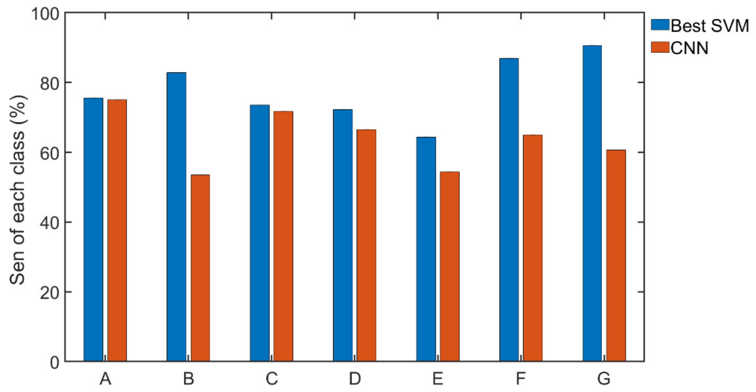
Figure 5 illustrates the recognition results of wind and rain AE signals are relatively poor, this may be caused by weak energy and the obvious white noise characteristics. and human voices are very random due to strong randomness. The normal with human voices in our catalog is also hard to distinguish, this is due to strong randomness in human voices, which can be presented in the spectral structure and time distribution of voice components.

Both CNN and KNN are basically satisfactory. Perhaps because this article did not perform special optimization processing on CNN, the advantages of CNN are still obvious, and there is no need to do too much preprocessing on features. From the perspective of execution time, SVM also has obvious advantages, and can achieve better results through the selection of parameters.

5. Discussion

An experiment confirmed our hypothesis that effective and quick recognition of transformer running states is possible by machine learning algorithms. Furthermore, the multi-classification experiments demonstrate that sounds with subtle differences can be discriminated by machine learning algorithms. In these experiments, the SVM classifier with 2DPCA presents good performance, which can be supported by the results shown in Table 2 and Table 3. The results show that the selection of kernel function for SVM and μ for PCA is important for acquiring the best performance. Different kernels and different μ not only have different influences on the sensitivity or accuracy of the fault detection, and can also have different effects in the time of recognition. As a general fault detection, PCA is also competent, but 2DPCA has a stronger ability to distinguish details, so it performs better in multi-classification problems. The randomness of speech and bird calls is too strong, and PCA will filter them out, so the effect is very poor. 2DPCA retains the details of the image, and the effect is very good.

In this paper, the real-time and online fault detection method of a substation power transformer based on the amplitude-frequency properties of the AE signals signal is proposed. It can be used as an effective means of fault detection of power transformers to assist the staff of substation in routine maintenance of power transformer, which can reduce the workload of manpower and detect problems early to avoid major accidents. In this study, from the results of the experiments, it can be seen that the amplitude-frequency-based method can be effectively applied in the fault detection of the sub-station power transformer by taking advantage of the AE signals emitted by the transformer. We can also see whether PCA combined with SVM or 2DPCA combined with SVM method, as long as suitable parameters are selected, can achieve satisfactory results. When the PCA combined with SVM is used and the linear is selected, the dimensionality reduction reconstruction threshold has little effect on the accuracy rate, but for other kernel functions, the performance becomes terrible when the dimensionality reduction reconstruction threshold is relatively small. However, when the 2DPCA combined with SVM is used, the choice of kernel function is more flexible than the PCA with SVM, but it is more easily affected by the feature dimensionality reduction reconstruction threshold whether under any kennel function. CNN method is easy to use and does not need to extract parameters manually, but it needs a long time training process and a large amount labeled data. In this work, the CNN does not show good performance as in other works perhaps because the labeled data is too small.

It should be noted that a failing transformer may not make a characteristic sound, or the sound may be hidden with other characteristic noises. This is a critical problem that we faced. Nonetheless, our work supplies a reference for discriminate different running state for transformers. Although the sounds in this work are not indicative of impending fault conditions, the resolving ability presented in our experiments can help for discriminate the true sound which is indicative of impending fault conditions. Many kinds of faults will emit characteristic noises, some are continuous, which can be considered suit to be identified adopting the method of this work. Some sounds, such as that given by the ionization effect on the high voltage terminals, may be constantly monitored is indicative of the progressive deterioration of the system. This noise can be distinguished in different phases (three phases of the three-phase system) which must be analyzed to understand which phase is failing. Although in three phases of the three-phase system, each phase will send different sound, compared to human speech, the sound has long stationary in each phase, which is still suitable treated by the methods introduced in this work. In human continuous speech recognition, HMM or LSTM are used to deal random time sequence with muti-states. Correspondingly for transformer sound, as long as three phases or more can be observed, the methods introduced in this work accompanied by the Majority vote, can be applied for solving the problem.

Due to the size of the power transformer being generally large, the AE signals of the various parts of the device spread in all directions, the AE signals intensity will inevitably be weaker in some directions. For the sound collection of the power transformer described in this paper, in the practical application, multiple microphones or acoustic receivers with spatial directivity can be deployed for acquiring more efficient information.

6. Conclusions

The aim of the study was to explore an appropriate machine learning method for monitor the transformer running state or detector the fault by taking advantage the AE signals. The experiment uses acoustic data from the transformer preprocessed and analyzed using the machine learning algorithms. The results confirm that efficient and quick detection of fault state or distinguish the different type of AE signals is possible. In the dichotomous data catalog for fault detection experiment, the best classifier achieved the sensitivity equal to 100%. Both the SVM with linear kernel PCA and SVM with RBF kernel 2DPCA have the optimal performance. In the multi-class data catalog for AE signals discrimination experiment, the best classifier achieved the average sensitivity equal to 88.37% and kappa equal to 82.40% when SVM with RBF kernel 2DPCA was used. These results were obtained with uneven sizes of labeled data in each category, which can be used as a reference for other small data volume multi-classification problems, in addition to sound detection of transformers. Although deep learning is very hot, in some cases, traditional methods such as SVM are still useful. This paper illustrates some advantages of traditional methods with examples, and gives a reference for parameter selection.

References

- Massagram, W.; Hafner, N.; Lubecke, V.; Boric-Lubecke, O. Tidal Volume Measurement Through Non-Contact Doppler Radar With DC Reconstruction. IEEE Sens. J. 2013, 13, 3397–3404. [Google Scholar] [CrossRef]
- Kaveh, S.; Norouzi, Y. Non-uniform sampling and super-resolution method to increase the accuracy of tank gauging radar. IET Radar Sonar Navig. 2017, 11, 788–796. [Google Scholar] [CrossRef]
- Lambert, S.M.; Armstrong, M.; Attidekou, P.S.; Christensen, P.A.; Widmer, J.D.; Wang, C.; Scott, K. Rapid Nondestructive-Testing Technique for In-Line Quality Control of Li-Ion Batteries. IEEE Trans. Ind. Electron. 2016, 64, 4017–4026. [Google Scholar] [CrossRef]
- Kreis, T. Application of Digital Holography for Nondestructive Testing and Metrology: A Review. IEEE Trans. Ind. Inform. 2015, 12, 240–247. [Google Scholar] [CrossRef]
- Moallemi, N.; ShahbazPanahi, S. A New Model for Array Spatial Signature for Two-Layer Imaging With Applications to Nondestructive Testing Using Ultrasonic Arrays. IEEE Trans. Signal Process. 2015, 63, 2464–2475. [Google Scholar] [CrossRef]
- Ricci, M.; Senni, L.; Burrascano, P. Exploiting Pseudorandom Sequences to Enhance Noise Immunity for Air-Coupled Ultrasonic Nondestructive Testing. IEEE Trans. Instrum. Meas. 2012, 61, 2905–2915. [Google Scholar] [CrossRef]
- Zhang, D.; Zhou, Z.; Sun, J.; Zhang, E.; Yang, Y.; Zhao, M. A Magnetostrictive Guided-Wave Nondestructive Testing Method with Multifrequency Excitation Pulse Signal. IEEE Trans. Instrum. Meas. 2014, 63, 3058–3066. [Google Scholar] [CrossRef]
- Sun, A.; Wu, Z.; Fang, D.; Zhang, J.; Wang, W. Multimode Interference-Based Fiber-Optic Ultrasonic Sensor for Non-Contact Displacement Measurement. IEEE Sens. J. 2016, 16, 5632–5635. [Google Scholar] [CrossRef]
- Chen, L.; Yang, X.; Fu, P.; Xu, Z.; Zhang, C. Novel Doppler approach to monitoring driver drowsiness. Electron. Lett. 2016, 52, 2011–2013. [Google Scholar] [CrossRef]
- Changhwan, C.; Byungsuk, P.; Seungho, J. The Design and Analysis of a Feeder Pipe Inspection Robot with an Automatic Pipe Tracking System. IEEE/ASME Trans. Mechatron. 2010, 15, 736–745. [Google Scholar] [CrossRef]
- Anami, B.S.; Pagi, V.B. Acoustic signal based detection and localisation of faults in motorcycles. IET Intell. Transp. Syst. 2014, 8, 345–351. [Google Scholar] [CrossRef]
- Silva, C.E.R.; Alvarenga, A.V.; Costa-Felix, R. Nondestructive testing ultrasonic immersion probe assessment and uncertainty evaluation according to EN 12668-2:2010. IEEE Trans. Ultrason. Ferroelectr. Freq. Control 2012, 59, 2338–2346. [Google Scholar] [CrossRef] [PubMed]
- Kong, W.; Hong, J.; Jia, M.; Yao, J.; Cong, W.; Hu, H.; Zhang, H. YOLOv3-DPFIN: A Dual-Path Feature Fusion Neural Network for Robust Real-time Sonar Target Detection. IEEE Sens. J. 2019, 20, 3745–3756. [Google Scholar] [CrossRef]
- Toffa, O.K.; Mignotte, M. Environmental Sound Classification Using Local Binary Pattern and Audio Features Collaboration. IEEE Trans. Multimed. 2020, 23, 3978–3985. [Google Scholar] [CrossRef]
- Ma, X.; Zhou, W.; Ju, F. Robust speech feature extraction based on dynamic minimum subband spectral subtraction. In Intelligent Computing in Signal Processing and Pattern Recognition; Lecture Notes in Control and Information Sciences; Springer: Berlin/Heidelberg, Germany, 2006; Volume 345, pp. 1056–1061. [Google Scholar]
- Salakhutdinov, R.; Tenenbaum, J.B.; Torralba, A. Learning with Hierarchical-Deep Models. IEEE Trans. Pattern Anal. Mach. Intell. 2013, 35, 1958–1971. [Google Scholar] [CrossRef] [Green Version]
- Pham, M.T.; Kim, J.M.; Kim, C.H. Intelligent Fault Diagnosis Method Using Acoustic Emission Signals for Bearings under Complex Working Conditions. Appl. Sci. 2020, 10, 7068. [Google Scholar] [CrossRef]
- Kim, J.Y.; Kim, J.M. Bearing Fault Diagnosis Using Grad-CAM and Acoustic Emission Signals. Appl. Sci. 2020, 10, 2050. [Google Scholar] [CrossRef] [Green Version]
- Kirby, M.; Sirovich, L. Application of the Karhunen-Loeve procedure for the characterization of human faces. IEEE Trans. Pattern Anal. Mach. Intell. 1990, 12, 103–108. [Google Scholar] [CrossRef] [Green Version]
- Yang, J.; Zhang, D.; Frangi, A.F.; Yang, J. Two-Dimensional PCA: A New Approach to Appearance-Based Face Representation and Recognition. IEEE Trans. Pattern Anal. Mach. Intell. 2004, 26, 131–137. [Google Scholar] [CrossRef] [Green Version]
- Zhou, B.; Khosla, A.; Lapedriza, A.; Oliva, A.; Torralba, A. Object detectors emerge in deep scene CNNs. ICLR’2015. arXiv 2015, arXiv:1412.6856.470. [Google Scholar]
- Ma, X.; Zhou, W.; Ju, F.; Jiang, Q. Speech Feature Extraction Based on Wavelet Modulation Scale for Robust Speech Recognition. In International Conference on Neural Information Processing; Springer: Berlin/Heidelberg, Germany, 2006; Volume 4233, pp. 499–505. [Google Scholar] [CrossRef]
- Ma, X.; Zhang, S.; Dong, Z.; Lu, H.; Li, J.; Zhou, W. Special acoustical role of pinna simplifying spatial target localization by the brown long-eared bat Plecotus auritus. Phys. Rev. E 2020, 102, 040401. [Google Scholar] [CrossRef] [PubMed]
- Altman, N.S. An introduction to kernel and nearest-neighbor nonparametric regression. Am. Stat. 1992, 46, 175–185. [Google Scholar]
- Bai, Y.Q.; Roos, C. A polynomial-time algorithm for linear optimization based on a new simple kernel function. Optim. Methods Softw. 2003, 18, 631–646. [Google Scholar] [CrossRef]
- Steinwart, I.; Hush, D.; Scovel, C. An Explicit Description of the Reproducing Kernel Hilbert Spaces of Gaussian RBF Kernels. IEEE Trans. Inf. Theory 2006, 52, 4635–4643. [Google Scholar] [CrossRef]
- Duda, R.O. Pattern Classification, 2nd ed.; Ricoh Innovations, Inc.: Menlo Park, CA, USA, 2001. [Google Scholar]
- Piczak, K.J. Environmental sound classification with convolutional neural networks. In Proceedings of the IEEE International Workshop on Machine Learning for Signal Processing, Boston, MA, USA, 17–20 September 2015. [Google Scholar]
- Librosa: v0.6.0. 2018. Available online: https://librosa.org/doc/main/changelog.html (accessed on 8 January 2022).
- Thompson, W.; Walter, S.D. A rEAPPRAISAL OF THE KAPPA COEFFICIENT. J. Clin. Epidemiol. 1988, 41, 949–958. [Google Scholar] [CrossRef]
- Chang, C.-C.; Lin, C.-J. LIBSVM: A Library for Support Vector MACHINES. Available online: http://www.csie.ntu.edu.tw/~cjlin/libsvm/ (accessed on 8 January 2022).