Article

Systematic Odometry Error Evaluation and Correction in a Human-Sized Three-Wheeled Omnidirectional Mobile Robot Using Flower-Shaped Calibration Trajectories

Robotics Laboratory, Universitat de Lleida, 25001 Lleida, Spain
*
Author to whom correspondence should be addressed.
Appl. Sci. 2022, 12(5), 2606; https://doi.org/10.3390/app12052606
Submission received: 25 January 2022 / Revised: 24 February 2022 / Accepted: 28 February 2022 / Published: 2 March 2022
(This article belongs to the Special Issue Trajectory Analysis, Positioning and Control of Mobile Robots)

Abstract

:
Odometry is a simple and practical method that provides a periodic real-time estimation of the relative displacement of a mobile robot based on the measurement of the angular rotational speed of its wheels. The main disadvantage of odometry is its unbounded accumulation of errors, a factor that reduces the accuracy of the estimation of the absolute position and orientation of a mobile robot. This paper proposes a general procedure to evaluate and correct the systematic odometry errors of a human-sized three-wheeled omnidirectional mobile robot designed as a versatile personal assistant tool. The correction procedure is based on the definition of 36 individual calibration trajectories which together depict a flower-shaped figure, on the measurement of the odometry and ground truth trajectory of each calibration trajectory, and on the application of several strategies to iteratively adjust the effective value of the kinematic parameters of the mobile robot in order to match the estimated final position from these two trajectories. The results have shown an average improvement of 82.14% in the estimation of the final position and orientation of the mobile robot. Therefore, these results can be used for odometry calibration during the manufacturing of human-sized three-wheeled omnidirectional mobile robots.

1. Introduction

Mobile robots have a huge range of potential applications in industrial, office and home environments. Autonomous mobile robots must be able to perform localization, mapping and navigation with reasonable levels of accuracy in order to successfully develop and complete their tasks. Localization methods consist of absolute or relative positioning methods [1,2]. Borenstein et al. [2] reviewed the most relevant mobile robot relative positioning methods based on internal data gathered by the mobile robot: odometry and inertial navigation, and the most relevant absolute positioning methods based on gathering external surrounding data.
Odometry is usually defined as a relative positioning method that uses the measures of the velocities of the wheels to estimate the position of the robot. Compared to other techniques, odometry is simple, affordable, and can be used in real-time, but as a relative positioning method it cumulates errors that may lead to inaccurate results. The improvement of odometry through proper calibration reduces the position errors and can contribute to lowering the costs of mobile robots by avoiding the use of precise external sensors.
In 1996, Borenstein et al. [3] introduced a benchmark test to measure the odometric accuracy of a mobile robot. This test, called University of Michigan Benchmark (UMBmark), consists on a bidirectional square path experiment in which a differential drive mobile robot performs a squared path in the clockwise and counterclockwise directions to avoid the compensation of odometry errors that might occur in unidirectional squared path experiments. The method first computes the contribution of errors caused by incorrect wheelbase (distance from the wheel to the center of the mobile robot) and by unequal wheel diameters. These errors are evaluated separately and then superimposed. In the case of a differential drive mobile robot, a wheelbase error causes pure rotation errors, which can be corrected by applying a correction factor to the wheelbase distances. The unequal wheel diameters error causes the robot to move on curved paths instead of straight trajectories. The radius of curvature of the real path can be computed to determine the ratio between the two-wheel diameters and compensate this systematic error. The application of the UMBmark provides a quantitative measure and corrects the systematic odometry errors, which allows comparison between different mobile robots. In summary, the results presented by Borenstein et al. [3] allowed an improvement of one order of magnitude in odometry accuracy.
An alternative to direct odometry calibration from the information gathered from the wheels is the application of data fusion from different sensors. Gargiulo et al. [4] estimated the mobile robot position and orientation by fusing information gathered from the wheels and an Inertial Measurement Unit (IMU). Zwierzchowski et al. [5] used a similar approach and included the information gathered from a vision system that measures the distance between the robot and custom markers located in the surrounding space. Xue et al. [6] fuses the information gathered from the wheels, an IMU and a 2D LIDAR in order to operate in diverse outdoor environments without any prior information. In a different approach, Palacin et al. [7] directly estimates the position and orientation of the mobile robot using the information provided by an onboard precise 2D LIDAR processed with simultaneous location and mapping (SLAM) [8]. In this case, the odometry was used as an initial estimation of the relative motion in order to improve the computational efficiency of SLAM. More recently, Xiao et al. [9] fused the information gathered from one IMU and two low-precision 2D LIDARs placed transversally to estimate the position and orientation of a mobile robot. However, the main disadvantage of using LIDARs is the cost of the sensor that is proportional to its measurement accuracy.
In the specific case of omnidirectional mobile robots, the determination of the odometry from the velocity gathered from the wheels has similar error sources but more complexity because of having more degrees of freedom in the motion [10]. In this direction, Maddahi et al. [11] proposed a method for the calibration of small three-wheeled omnidirectional mobile robots in order to reduce positioning errors. The procedure was based on the determination of two corrective indices for the inverse kinematic matrix used by the odometry to estimate the position of the robot. This method consists of: (1) determining the kinematic equations of the robot; (2) registering of the motion of the non-calibrated robot moving along a straight line; (3) evaluating the longitudinal error ( x e ), lateral error ( y e ) and angular error ( θ e ) between the target and real trajectory positions; and (4) the computation of some corrective indices. This method corrects the longitudinal ( x e ) and lateral ( y e ) errors separately. First, a lateral corrective matrix, which compensates the lateral position error of the robot ( y e ), is computed from the angular error of the robot ( θ e ). Secondly, a longitudinal corrective factor used to eliminate the longitudinal position error ( x e ) is computed from the longitudinal ( x e ) and lateral errors ( y e ). Finally, both indices are multiplied with the Jacobian matrix used by the odometry to estimate the velocities of the wheels. The corrected Jacobian matrix is then used to compute the corrected angular velocities of the wheels. This proposal was experimentally validated with different trajectories, comparing the positioning errors before and after calibration. Results showed significant improvements: the root mean square (RMS) of the positioning error was reduced between 68% and 91% in double-squared, double-triangle and circular paths. In this case, the analysis of the trajectories and positioning errors evidenced that the improvement depends on the type of trajectory being accurate in straight trajectories and less accurate in the case of combined straight and curved trajectories.
Similarly, Lin et al. [12] presented an odometry calibration method for medium-size three-wheeled omnidirectional mobile robots based on the correction of its kinematic model. The method consists on gathering discrete position and orientation data and estimating the kinematic parameters by a least square method. The information required by this process is the initial and final positions of the mobile robot through N experiments (multiple data sets). This proposal is not limited by the relationship between the parameters used in the kinematic equations, so the obtained kinematic model may better describe the odometry of the mobile robot. Lin et al. [12] verify their calibration method by comparing the ideal trajectory and the trajectories before and after calibration.
In a similar direction, Li et al. [13] presented a method for the reduction of positioning errors of four-wheel omnidirectional mobile robots using Mecanum wheels. The main problem of four-wheel omnidirectional mobile robots is wheel slippage, so this method analyzed the kinematic model of the mobile robot and provides a velocity compensation matrix to reduce the errors of the robot motion caused by wheel slippage. This compensation matrix was validated using virtual simulations and experimental tests. Results showed that the compensation matrix reduces the errors of robot motions caused by wheel slippage, improving the motion accuracy of the system. However, Li et al. [13] concluded that this velocity compensation matrix must be adjusted according to the velocity of the mobile robot. Alternatively, Lu et al. [14] fused the information gathered from an IMU, a gyroscope and encoders to estimate the odometry of a mobile robot using four Mechanum wheels to estimate the estimated odometry on a floating ground.
More recently, Savaee et al. [15] proposed a simplification of the method presented by Maddahi et al. [11]. The new method uses the kinematic model of a three-wheeled mobile robot and computed a corrected Jacobian matrix to reduce the effects of systematic errors in the odometry. This method used a genetic algorithm to find the matrix elements of a corrected Jacobian matrix, which are called Effective Kinematic Parameters (EPKs). This new method consists of: (1) creating a model of the virtual robot and of the systematic errors; (2) performing simulation tests with the virtual robot; (3) performing experimental tests with a real robot; (4) comparing both results to estimate the EPKs and redefine the Jacobian matrix of the mobile robot. In this case, the simulation and experimental tests consist of two robot translations along straight paths and one rotation about itself, and the calculated EPKs are used to correct the angular velocities of the wheels. This procedure was verified with a three-wheeled omnidirectional mobile robot performing different paths. In general, the evaluation of tracking errors in offline analysis has the advantage of avoiding local minimum in complex parametric nonlinear systems [16].

New Contribution

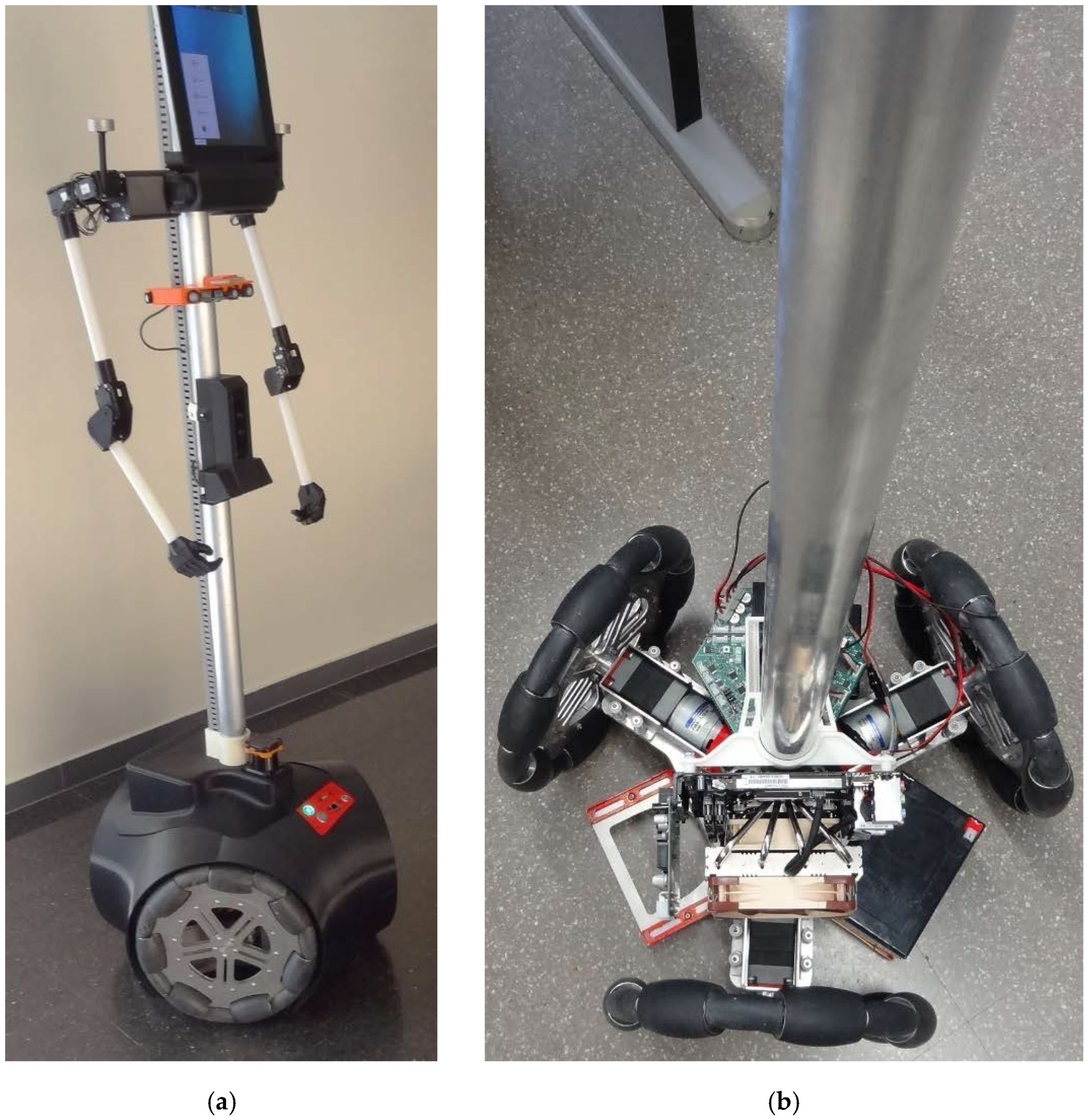
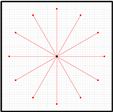
The new contribution of this paper is the proposal of a combination of 36 straight and curved calibration trajectories for systematic odometry error evaluation and correction in a three-wheeled omnidirectional mobile robot. This procedure has been empirically applied and validated in a real human-sized three-wheeled omnidirectional mobile robot of 1.760 m and 30 Kg (Figure 1). These 36 calibration trajectories have been proposed as a representative test-bench of the infinite trajectories that can be performed by an omnidirectional mobile robot, which together depict a characteristic flower-shaped figure. The calibration procedure implemented requires the registering of the real odometry and ground truth trajectories generated while performing each calibration trajectory. Finally, the odometry of each calibration trajectory is recomputed offline to iteratively adjust the effective values of the kinematic parameters of the mobile robot in order to match the odometry with the ground truth trajectory. This paper has evaluated different matching strategies using different sets of calibration trajectories. The best matching between the odometry and ground truth trajectories has been obtained using genetic algorithms and 5 repetitions of each one of the proposed 36 calibration trajectories. The fitting results of the kinematic parameters have been validated by performing 5 additional repetitions of the 36 calibration trajectories.
This new contribution was inspired in Batlle et al. [17], who proposed the use of four curved calibration trajectories, and in Maddahi et al. [11], who calibrated the odometry with straight paths but concluded that the percentage of error correction depends on the type of the path. The new contribution is the proposal of a complete set of straight and curved calibration trajectories which together depict a characteristic flower-shaped figure. This new contribution is also inspired in the work of Savaee et al. [15] that used genetic algorithms to adjust the kinematic matrix of a three-wheeled mobile robot although without comparing the results obtained with other minimization alternatives. This proposal will apply the same methodology proposed by Lin et al. [12], based on the comparison of the initial and final positions of the mobile robot through N experiments to directly evaluate the odometry improvement achieved. Finally, as an alternative to Savaee et al. [15] and Lin et al. [12], this new proposal adjusts the value of the kinematic parameters of the mobile robot (radii of the wheels, distance from the wheel to the center of the mobile robot and angular orientation of the wheels) instead of directly adjusting the values of the kinematic matrix, allowing a direct physical interpretation of the fitting results obtained.

2. Materials and Methods

The material used in this paper is the omnidirectional mobile robot APR-02 (Figure 1). The methods used in this paper are the odometry of the mobile robot and two nonlinear minimization procedures based on gradient search and genetic algorithm. These two minimization methods will be applied to calibrate the odometry of the mobile robot.

2.1. Omnidirectional Mobile Robot APR-02

The omnidirectional mobile robot APR-02 is the second family prototype designed under the project concept titled Assistant Personal Robot (APR). The goal of the APR project is the final implementation of a versatile human-sized mobile robot that can be applied to develop different assistance services, for example, to supporting older people with mobility limitations [18]. The main difference of the APR concept with other comparative mobile robot designs [19] is the use of an omnidirectional motion system based on three omnidirectional wheels in which the free rollers are aligned with the rotation plane of the wheels. The main advantage of this design using three wheels is the minimization of wheel slippage regardless of the motion implemented by the mobile robot [20].
Figure 1a shows the omnidirectional mobile robot APR-02 and Figure 1b shows a detail of its omnidirectional motion system based on the use of three omnidirectional wheels. The main sensor of the APR-02 is a precise onboard 2D LIDAR Hokuyo UTM-30LX either placed horizontally or tilted down [7] to directly detect small obstacles laying on the ground or holes or stairs in front of the mobile robot, and for SLAM [8]. The APR-02 has been used as a research tool in some recent applications. In [21] an alternative omnidirectional wheel design was proposed to foster future outdoor applications. In [22] the motors and encoders of the mobile robot were analyzed in order to improve the measurement of the estimated angular velocity of the wheels.
The trajectory of the mobile robot APR-02 is established by its path-planning algorithm that continuously updates the target motion vector ( v , α , ω , t r ) of the mobile robot [20] accordingly to a task or objective. This target motion vector is converted into individual target angular rotational velocities of the three wheels ( ω M a , ω M b , ω M c ) which are then applied to the PID controllers of the DC motors driving these three wheels in order to implement the planned motion.

2.2. Odometry Trajectory

Odometry is a simple and practical method that provides a periodic real-time estimation of the relative displacement of a mobile robot based on the measurement of the angular rotational speed of its wheels. Odometry estimation is valid in the case of non-slippage wheel conditions in which wheel revolutions can be translated into linear displacement relative to the floor. The advantage of an omnidirectional mobile robot using three optimal omnidirectional wheels is that the wheels do not have motion constrains and do not require slippage in order to implement any motion trajectory [20].
The kinematics and the odometry of the mobile robot APR-02 are described in [20]. Figure 2 presents the parametric definition of the omnidirectional motion system based on three omnidirectional wheels (Figure 2a) and a detail of the parameters of one wheel (Figure 2b). The main parameters are: the position of the mobile robot ( x , y , θ ) referred to the fixed world frame ( X W , Y W ) , the motion command of the robot ( v , α , ω ) , the angular velocities of the wheels ( ω a , ω b , ω c ) , the linear velocities of the wheels ( V a , V b , V c ) , the radii of the wheels ( r a , r b , r c ) , the distance between the center of the robot and each wheel ( R a , R b , R c ) and the angular orientation of each wheel ( δ a , δ b , δ c ) referred to the mobile robot frame ( X R , Y R ) .
The odometry procedure uses the instantaneous estimate of the current angular velocities of the three wheels, a ,   b ,   c , available as a vector sequence ( ω a ( k ) , ω b ( k ) , ω c ( k ) ) in order to estimate the instantaneous position of the mobile robot ( x ( k ) , y ( k ) , θ ( k ) ) in the world frame ( X W , Y W ) . The relation between the instantaneous estimation of the angular velocities of the wheels ( ω a ( k ) , ω b ( k ) , ω c ( k ) ) and the instantaneous robot velocity ( v x ( k ) , v y ( k ) , ω ( k ) ) in the world frame ( X W , Y W ) can be summarized as [20]:
[ ω a ( k ) ω b ( k ) ω c ( k ) ] = [ 1 / r a 0 0 0 1 / r b 0 0 0 1 / r c ] · [ s i n ( δ a ) c o s ( δ a ) R a s i n ( δ b ) c o s ( δ b ) R b s i n ( δ c ) c o s ( δ c ) R c ] · [ c o s ( θ ( k 1 ) )   s i n ( θ ( k 1 ) ) 0 s i n ( θ ( k 1 ) ) c o s ( θ ( k 1 ) ) 0 0 0 1 ] · [ v X ( k ) v Y ( k ) ω ( k ) ] W o r l d
Which includes a rotation matrix R ( θ ) and a compact kinematic matrix M that defines the overall kinematics of the mobile robot:
R ( θ ) = [ cos ( θ )   sin ( θ ) 0 sin ( θ ) cos ( θ ) 0 0 0 1 ]
M = [ s i n ( δ a ) / r a   c o s ( δ a ) / r a R a / r a s i n ( δ b ) / r b c o s ( δ b ) / r b R b / r b s i n ( δ c ) / r c c o s ( δ c ) / r c R c / r c ]
Equation (1) can be arranged to update the current position of the mobile robot   ( x ( k ) , y ( k ) , θ ( k ) ) in the world frame ( X W , Y W ) based on the new estimate of the current angular velocities of the three wheels of the mobile robot ( ω a ( k ) , ω b ( k ) , ω c ( k ) ) and the time lapse Δ t between the samples   k 1 and k , which in the mobile robot APR-02 coincides with the sampling time T of its proportional-integral-derivative (PID) motor controllers, Δ t = T = 10   m s :
[ x ( k ) y ( k ) θ ( k ) ] W o r l d = [ x ( k 1 ) y ( k 1 ) θ ( k 1 ) ] W o r l d + T · R ( θ ( k 1 ) ) 1 · M 1 · [ ω a ( k ) ω b ( k ) ω c ( k ) ]
where R 1 ( θ ) is the inverse of the rotation matrix defined by the previous instantaneous angular orientation of the mobile robot θ ( k 1 ) :
R ( θ ) 1 = [ cos ( θ )   sin ( θ ) 0 sin ( θ ) cos ( θ ) 0 0 0 1 ]
And M 1 is the inverse of the compact kinematic matrix M :
M 1 = 1 R a sin ( δ b δ c ) R b sin ( δ a δ c ) + R c sin ( δ a δ b ) ·                    [ r a ( R b cos ( δ c ) R c cos ( δ b ) ) r b ( R a cos ( δ c ) R c cos ( δ a ) ) r c ( R a cos ( δ b ) R b cos ( δ a ) ) r a ( R b sin ( δ c ) R c sin ( δ b ) ) r b ( R a sin ( δ c ) R c sin ( δ a ) ) r c ( R a sin ( δ b ) R b sin ( δ a ) ) r a sin ( δ b δ c ) r b sin ( δ a δ c ) r c sin ( δ a δ b )

2.3. Odometry Errors: Systematic and Non-Systematic

The main disadvantage of odometry is its unbounded accumulation of errors in the evaluation of the trajectory of a mobile robot (see Equation (4)). The error sources that cause inaccuracies in the determination of the odometry depend largely on the type of terrain practiced by the mobile robot [3], and are classified as systematic and non-systematic. In general, the concept of odometry calibration is focused on the minimization of systematic errors because they remain constant during the displacement. In general, the errors affecting the orientation of the mobile robot have the worst cumulative effects because once they are incurred they grow into lateral position errors [23,24].

2.3.1. Systematic Odometry Errors

Systematic odometry errors are usually invariant because they are caused by inaccuracies and imperfections in the mechanical implementation of the robot, such as mismatches between the nominal and effective parameters, or by limited sensors capabilities, resolution and sampling rate. Borenstein et al. [3] concluded that the systematic errors that have greater effects in the odometry are caused by unequal wheel diameters and placement accuracy in the wheelbase, which is the distance between the point of contact of the wheel with the floor and the center of the robot. Systematic errors accumulate constantly, so they are usually the main contributors to positioning errors in smooth indoor terrains.

2.3.2. Non-Systematic Odometry Errors

Non-systematic odometry errors are not possible to predict, because they are originated by unpredictable features of the environment such as terrain irregularities, terrain obstacles, structural wheel slippage during specific motions, wheel slippage originated by the terrain conditions, or the application of external forces to the mobile robot. However, this paper is applied to a mobile robot operating in perfect flat indoor terrains, so the assumption is that the motion will not be affected by non-systematic odometry errors.

2.4. Systematic Odometry Error Sources in a Three-Wheeled Omnidirectional Mobile Robot

The exact theoretical value of the inverse of the compact kinematic matrix M 1 computed with the nominal values of the kinematic parameters ( R a = R b = R c = 0.195   m , r a = r b = r c = 0.148   m and δ a = 60°, δ b = 180°, δ c = 300°) evaluated using a standard double precision floating-point format (IEEE 754-1985: 4-bytes data or 64-bit data, precision 1.11 × 10⁻¹⁶ [25]) is:
M 1 = [ 0.0854478398400646             0.0000000000000000       0.0854478398400646       0.0493333333333333       0.0986666666666667       0.0493333333333333       0.2529914529914529             0.2529914529914529       0.2529914529914529 ]
The simple numerical representation of the exact values of the coefficients of the inverse of the compact kinematic matrix M 1 of the mobile robot APR-02 intuitively indicates that any inaccuracy in the values of the kinematic parameters may cause a large impact in the generation of systematic errors during the cumulative evaluation of the odometry (see Equation (4)).
In a real mobile robot application, the effective values of the kinematic parameters R a ,   R b ,   R c ,   r a ,   r b ,   r c , δ a , δ b , δ c can differ from the nominal values due to imprecisions in the manufacturing process and then originate systematic errors in the cumulative computation of the odometry of a mobile robot. The following figures are proposed to graphically illustrate the uncertainties that appear in the determination of the exact or effective value of the kinematic parameters of a real mobile robot. Figure 3 shows two views of one omnidirectional wheel of the motion system of the mobile robot APR-02 and a representation of its radius r a . Even in this case in which the wheel cover is thin and smooth, the accurate determination of the radius of the wheel is very difficult and will have some uncertainty because of the difficulty in the estimation of the point of contact with the floor [26]. Similarly, Figure 4 shows two views of the representation of the distance to the center of the mobile robot. Figure 4a shows the effect of a vertical wheel misalignment (exaggerated in this case) and Figure 4b the effect caused by the point of contact with the floor. Finally, Figure 5 shows two views of the effect of angular wheel misalignment that can be caused by the application of non-uniform pressure to the screws that hold the motor to the wheelbase through a rubber piece designed to absorb vibrations. These figures clearly reveal that manufacturing inaccuracies and assembly imprecisions will originate crossed systematic errors in the odometry of the omnidirectional mobile robot.
Finally, Table 1, Table 2 and Table 3 show the analytic determination of the sensitivity of the kinematic matrix M 1 to the kinematic parameters of the wheels, computed form Equation (6). These tables show very high sensitivities in the array values of M 1 , a matrix that is used to cumulatively update the position and location of the mobile robot 100 times per second (See Equation (4)). In the case of the distance from the center of the robot to each wheel, the maximum individual sensitivity of M 1 is as high as 0.43 mm/s for each millimeter of error in the determination of the real value of ( R a , R b , R c ) . In the case of the radii of the wheels, the maximum individual sensitivity of M 1 is as high as 1.70 mm/s for each millimeter of error in the determination of the real value of ( r a , r b , r c ) . Finally, in the case of the angular orientation of each wheel, the maximum individual sensitivity of M 1 is 0.14 mm/s for each angular arc degree error in the determination of the real value of ( δ a , δ b , δ c ) .

2.5. Ground Truth Trajectory

The calibration procedure proposed in this work requires the development of several motion experiments conducted in a controlled, clean and structured area, without obstacles on the floor and with plain and clean surrounding walls. During these motion experiments the odometry and the ground truth (or real) trajectory of the mobile robot are registered for offline calibration analysis. The trajectory estimated with the odometry is based on relative onboard information that is prone to cumulative systematic errors (see Section 2.4). The trajectory estimated from the precise information provided by the onboard LIDAR (providing 1.081 points per scan and a radial distance range up to 30 m) and processed with SLAM [8] is assumed as the ground truth trajectory of the mobile robot [20] because the absolute LIDAR information gathered in this clean conditions is not prone to systematic errors. The trajectory estimated with the odometry is based on relative onboard information that is prone to cumulative systematic errors (see Section 2.4) while the ground truth trajectory estimated with the precise onboard LIDAR is based on an absolute description of the structured environment around the mobile robot that is not prone to systematic errors. This procedure to obtain the ground truth trajectory was used previously in [20]. In case an accurate onboard LIDAR is not available, it will be necessary to obtain the ground truth trajectory using other means such as an external laser tracker [27,28] or external cameras [29].
Figure 6a shows a representation of the odometry and ground truth trajectories, which are usually different because of the existence of systematic odometry errors. The values represented are: the starting point of the mobile robot ( x i ,   y i ,   θ i ) , the motion command applied M = ( v , α ,   ω , t r ) , the true final position and orientation estimated with SLAM ( x g t f ,   y g t f ,   θ g t f ) , and the final position and orientation of the mobile robot estimated with the odometry ( x f ,   y f ,   θ f ) . In each motion experiment the mobile robot also registers all intermediate information needed to replicate the offline computation of the odometry and ground truth trajectories in order to perform the calibration of the odometry. The information registered is (see Figure 6b): a vector containing the sequence of instantaneous angular velocities of the three wheels and the elapsed time E ( k = 1 n ) = [ t ( k ) , [ ω a ( k ) , ω b ( k ) , ω c ( k ) ] ] , where n is the number of velocity samples available; a vector containing the position of the mobile robot estimated by the odometry O ( k = 1 n ) = [ t ( k ) , [ x ( k ) , y ( k ) , θ ( k ) ] ] ; and a vector containing the ground truth position G T ( p = 1 m ) = [ t ( p ) , [ x g t ( p ) , y g t ( p ) , θ g t ( p ) ] ] estimated with SLAM. Please note that t ( k ) is the time in which a new estimation of the instantaneous angular velocities of the wheels   E ( k ) is provided by the encoder. This time can be computed as t ( k ) = k · T or t ( k ) = t ( k 1 ) + T , where T is the sampling time of the PIDs; in the APR-02 this value is T = 10   ms . The odometry information O ( k ) is computed from E ( k ) , so it is defined by the same time sequence   t ( k ) . Alternatively, t ( p ) is the time in which a new raw scan L ( p ) is provided by the LIDAR. This time can be computed as t ( p ) = t ( p 1 ) + D p , where D p ranges from 200 ms to 300 ms depending on the time required by the control system of the mobile robot to apply SLAM and estimate G T ( p ) . This variation is because the control system waits to request a new LIDAR scan until the SLAM procedure finishes, so this time lapse will be different depending on the time needed to apply SLAM from the raw LIDAR scans.
The hypothesis of this paper is then that the odometry trajectory will be correct and exact when this trajectory matches the ground truth (real) trajectory of the mobile robot.
Figure 7 shows the final position results obtained when the mobile robot APR-02 repeats the same calibration trajectory five times, starting each trajectory with the same initial position and angular orientation. Figure 7 represents the zoomed information of the planned final destination of the mobile robot (black dot and line) when the mobile robot completes a simple straight trajectory, the ground truth trajectory (orange dotted line) and ground truth final position and orientation of the mobile robot (orange circle and line), and the trajectory (green dotted line) and final mobile robot position and orientation estimated with the odometry (green square and line). The results of Figure 7 reveal the existence of systematic differences between the odometry and ground truth trajectories. This paper proposes the reduction of such differences by applying an iterative calibration procedure to the kinematic parameters used to estimate the odometry of the mobile robot APR-02.

2.5.1. Distance and Angular Errors during a Trajectory

The determination of the distance and angular errors between the odometry trajectory points O ( k = 1 n ) and the ground truth trajectory points G T ( p = 1 m ) require the subsampling of the original odometry trajectory in order to have an odometry trajectory vector with the same length as the ground truth vector. The subsampled odometry trajectory vector O S S ( p = 1 m ) = [ t ( p ) , [ x ( p ) , y ( p ) , θ ( p ) ] ] is then obtained by searching for the nearest t ( k ) and t ( p ) values (see Figure 6b). The distance and angle error vectors are then computed as:
d i s t a n c e e r r o r ( p ) = ( x g t ( p ) x ( p ) ) 2 + ( y g t ( p ) y ( p ) ) 2
a n g l e e r r o r ( p ) = ( θ g t ( p ) θ ( p ) ) 2

2.5.2. Maximum Error in a Trajectory

The determination of the maximum distance and angular error between the odometry and ground truth trajectory is obtained from the distance error vector and the angle error vector, respectively, using:
M a x i m u m E r r o r D i s t a n c e = max ( d i s t a n c e e r r o r ( p = 1 m ) )
M a x i m u m E r r o r A n g l e = max ( a n g l e e r r o r ( p = 1 m ) )

2.5.3. RMS Error in a Trajectory

The determination of the Root Mean Square error (RMSE) that summarizes the differences between the odometry and ground truth trajectory are computed using:
R M S E d i s t a n c e = p = 1 m ( d i s t a n c e e r r o r ( p ) 2 ) m
R M S E a n g l e = p = 1 m ( a n g l e e r r o r ( p ) 2 ) m

2.5.4. Cost Function Summarizing Trajectory Differences

The cost function used in this paper to summarize in one single value C F the overall differences (position and angular orientation) between the odometry and ground truth trajectories is computed from the final position of the mobile robot using:
C F = ( x g t f x f ) 2 + ( y g t f y f ) 2 + ( θ g t f θ f ) 2
This cost function value C F will be used to guide the iterative odometry calibration procedure in order to tune the effective kinematic parameters of the mobile robot. This cost function was also used by Savaee et al. [15] to calibrate the effective kinematic parameters of a comparable omnidirectional mobile robot. This cost function implicitly applies the same weights to a final positioning with a distance error of 1 m or an angular arch error of 1°. We have selected this cost function because a small angular error usually has a large cumulative effect in the odometry of an omnidirectional mobile robot.

2.6. Iterative odometry Calibration Procedure

This paper proposes the application of an iterative calibration procedure to tune or adjust the effective value of the kinematic parameters of the mobile robot:   R a ,   R b ,   R c ,   r a ,   r b ,   r c , δ a , δ b , δ c , used to compute the M 1 matrix. These kinematic parameters have been described in Section 2.2 and represented graphically in Figure 2. The planned result of the iterative calibration procedure is a better match between the odometry and ground truth mobile robot trajectories.
Figure 8 depicts the flowchart of the iterative odometry calibration procedure. The iterative process starts with the nominal or theoretical values of the kinematic parameters of the mobile robot ( R a , R b , R c ,   r a , r b , r c ,   δ a , δ b , δ c ) , which are used to compute a first estimation of the M 1 matrix. Then, the iterative process uses the initial position and orientation of the mobile robot ( x i , y i , θ i ) and the sequence of angular rotational velocities of the wheels obtained from the encoders E ( k = 1 n ) = [ t ( k ) , [ ω a ( k ) , ω b ( k ) , ω c ( k ) ] ] to compute the odometry trajectory O ( k = 1 n ) of the mobile robot and estimate the final position and angular orientation of the mobile robot ( x f , y f , θ f ) = O ( k = n ) . Then, the cost function is used to compare this estimate of final position and orientation of the mobile robot ( x f , y f , θ f ) with its true position and orientation ( x g t f ,   y g t f ,   θ g t f ) = G T ( p = m ) .
The iterative minimization function evaluates the cost function and decides between repeating the loop with new values of the kinematic parameters or stopping the iterative minimization search. The final result of this iterative procedure is an improved or corrected M 1 matrix ready to better estimate the odometry of the mobile robot APR-02. The nonlinear minimization functions evaluated in this paper are based on gradient search and genetic algorithms (GA). In both cases, the inputs and genome of the minimization functions are the initial values of the kinematic parameters p a r a m i defined as:
p a r a m i = ( 0.195 ,   0.195 ,   0.195 ,   0.148 ,   0.148 ,   0.148 ,   60.000 ,   180.000 ,   300.000 )
And the upper ( p a r a m u b ) and lower ( p a r a m l b ) bounds proposed to guarantee the physical interpretation of the results:
p a r a m u b = ( 0.220 ,   0.220 ,   0.220 ,   0.158 ,   0.158 ,   0.158 ,   62.000 ,   182.000 ,   302.000 ) p a r a m l b = ( 0.170 ,   0.170 ,     0.170 ,   0.138 ,   0.138 ,   0.138 ,   58.000 ,   178.000 ,   298.000 )
The specific search functions used in this paper are:
Fmin search function. The implementation of a gradient search nonlinear minimization to calibrate the odometry is based on the Matlab function fmincon.m, which is a nonlinear multivariable function that attempts to iteratively find the local unconstrained minimum of an objective multivariate cost function summarized in a value C F evaluated within specific bounds. In this calibration application, the search will use p a r a m i as the initial population and p a r a m l b and p a r a m u b as the lower and upper bounds of the iterative search. The stopping criteria of this iterative search is a change in C F less than the default value of the parameter StepTolerance (10−10) with a maximum constraint violation less than the default value of the parameter Constraint Tolerance (10−6) before reaching the maximum number of iterations that is usually defined as the number of variables of p a r a m i multiplied by 100 (900).
GA search function. The implementation of a genetic algorithms (GA) minimization to calibrate the odometry is based on the Matlab function ga.m, which will attempt to iteratively find the local unconstrained minimum of an objective multivariate cost function summarized in a value C F evaluated within specific bounds. The inputs and outputs of the iterative search are the same as in the previous function. The initial population and bounds for the GA algorithm are defined using the Matlab function gaoptimset.m in the parameters InitialPopulation and PopInitRange. This iterative search stops if the average relative change in the best fitness of the cost function C F is less than or equal to the default value of the parameter FunctionTolerance (10−6).

3. Systematic Odometry Error Evaluation and Correction

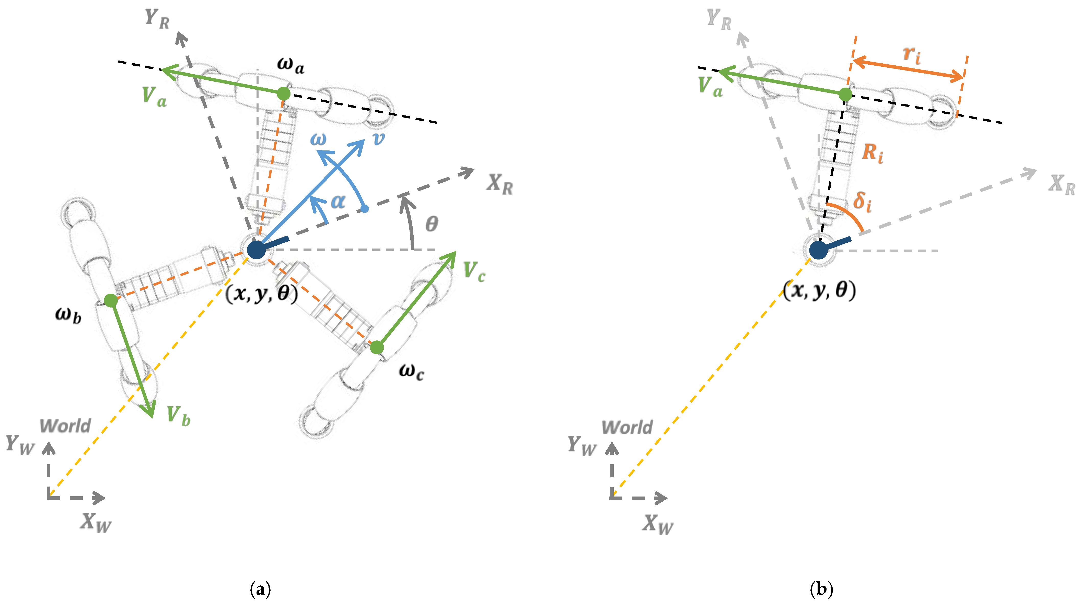
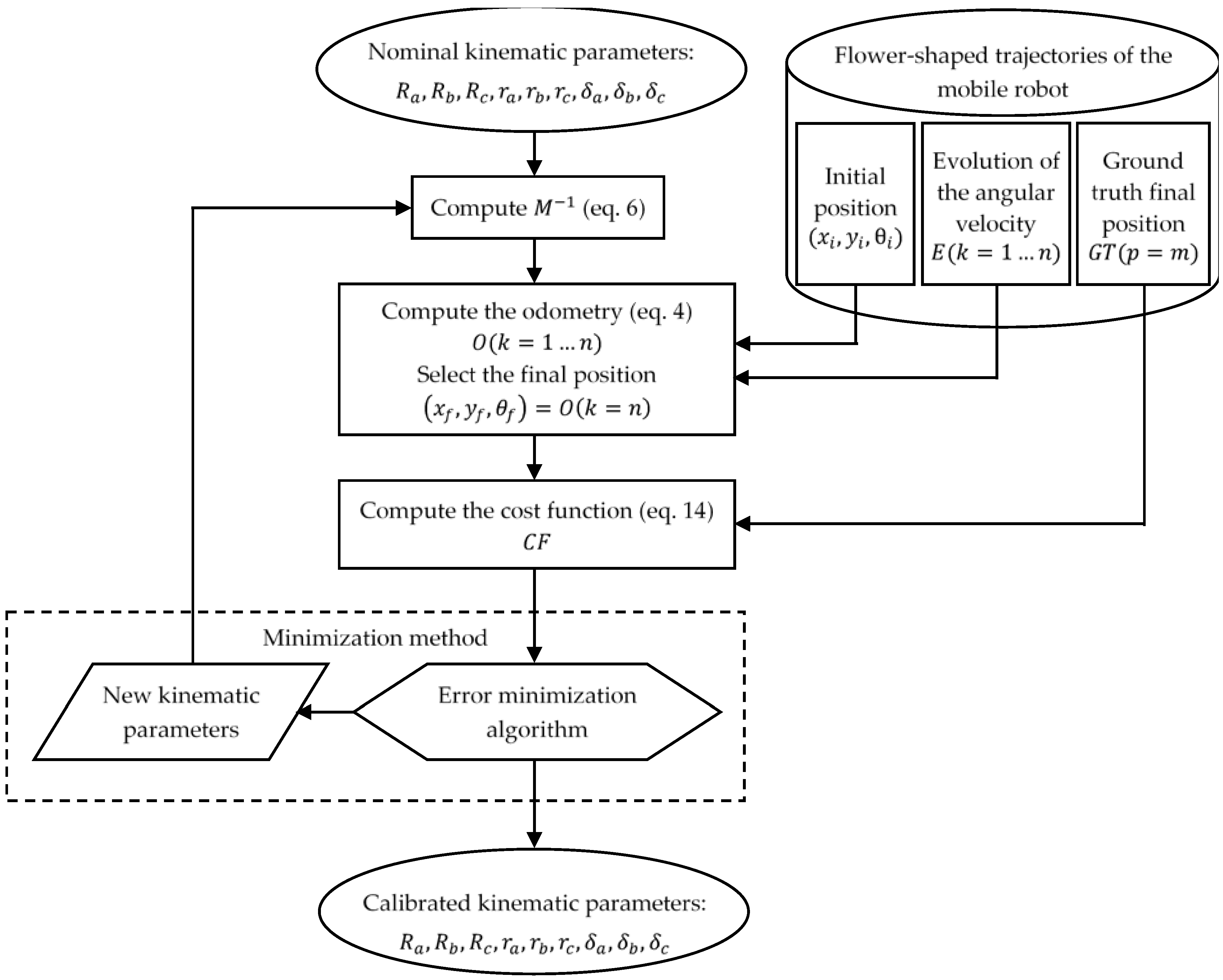
The procedure proposed in this paper to systematically evaluate and correct the systematic odometry errors of the omnidirectional mobile robot APR-02 is based on the definition of 36 individual calibration trajectories which together depict a flower-shaped figure, on the measurement of the odometry and ground truth trajectory in each calibration trajectory, and on the application of several strategies to iterative adjustment of the effective value of the kinematic parameters to match the odometry and the ground truth trajectories registered in these 36 calibration trajectories. The implementation of the 36 trajectories that define the flower-shaped figure is proposed as a representative test-bench of the infinite trajectories that can perform this omnidirectional mobile robot. In this paper, each calibration trajectory has been repeated 10 times; with a total of 360 registered trajectories. Five repetitions will be used to calibrate the effective value of the kinematic parameters and Five repetitions will be used to validate the results.

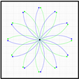
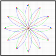
3.1. Calibration Trajectories Depicting a Characteristic Flower-Shaped Figure

This paper proposes the improvement of the odometry of the omnidirectional mobile robot APR-02 using a set of specific individual calibration trajectories that globally depict a characteristic flower-shaped figure. Figure 9 shows the proposed trajectories and Table A1 (listed in Appendix A) presents the motion command required to implement each calibration trajectory and the values of the corresponding target angular rotational velocities of the wheels required to implement each trajectory that will be specific for each mobile robot type.
The target angular velocities of the wheels shown in Table A1 (Appendix A) are in revolutions per minute (rpm) because this unit is normally used by the PIDs controlling the angular rotational velocity of the motors of the mobile robot. The calibration trajectories comprise straight displacements (
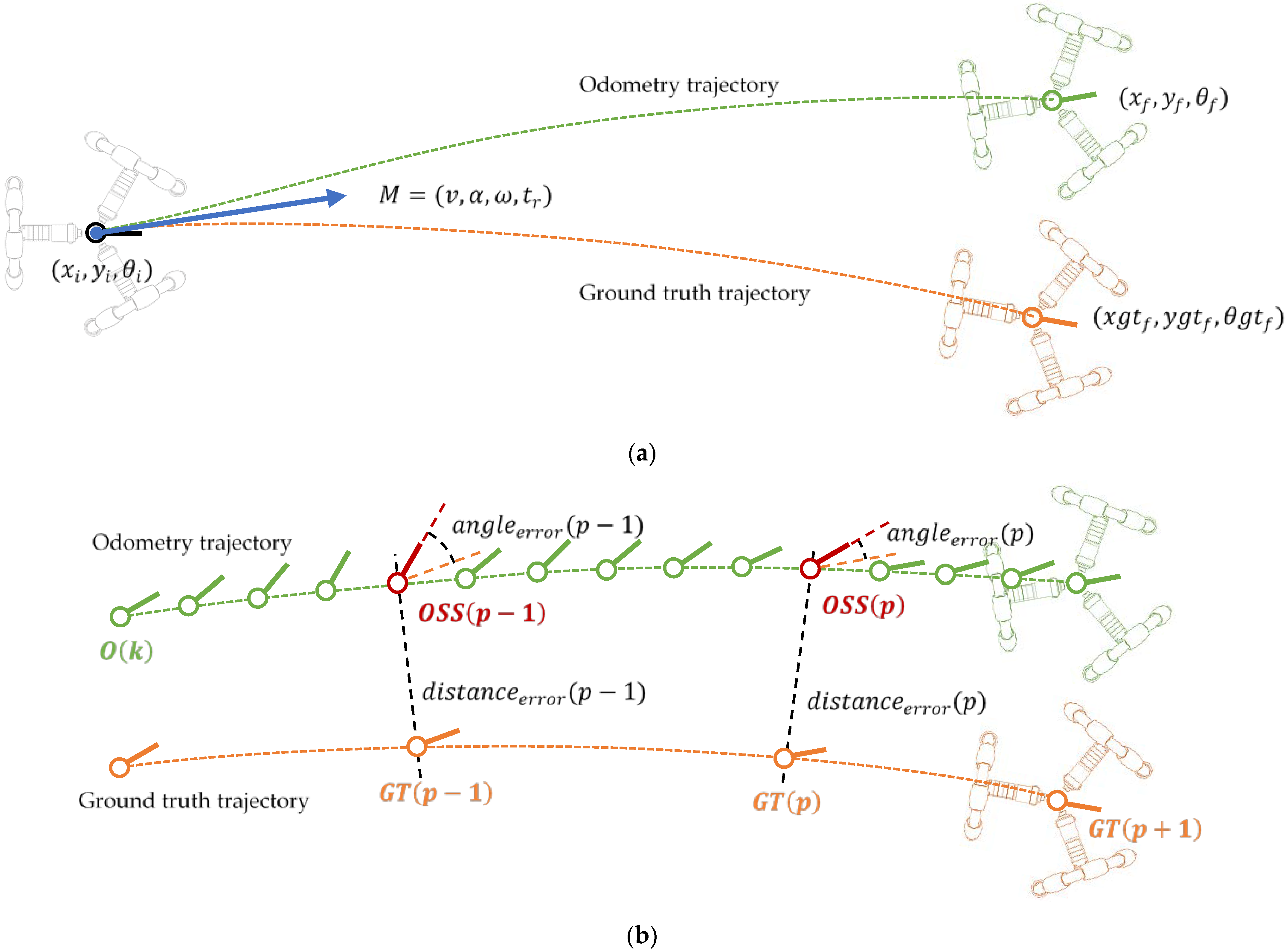
Figure 9, red line labeled with an R followed with a number), clockwise displacements (blue line labeled with a B followed with a number), and counterclockwise displacements (green line labeled with a G followed with a number). These 36 combinations of angular rotational velocities of the wheels are a short representation of the infinite set of possible motion combinations. The linear displacement of all trajectories has been limited to 1 m in order to generate a characteristic and easy to remember flower-shaped figure. In this paper, each trajectory has been repeated and registered 10 times in a total of 360 trajectory experiments. Each trajectory register contains the sequence of instantaneous angular velocities of the three wheels E ( k = 1 n ) , where n is the number of samples available; the vector containing the position of the mobile robot estimated by the odometry O ( k = 1 n ) ; and the vector containing the ground truth position G T ( p = 1 m ) estimated by the SLAM procedure.
The adequacy of the trajectories proposed in Figure 9 to the calibration of the odometry mobile robot APR-02 will be evaluated in the following section.

3.2. Odometry Calibration Strategies and Results

The odometry calibration strategies tested in this paper are based on analysis of the calibration trajectories proposed in Figure 9. The iterative calibration procedure used has been previously described in Section 2.6. In summary, this iterative calibration gets the registered calibration trajectories and iteratively adjusts the values of the effective kinematic parameters to globally match the odometry and ground truth trajectories.
Table 4 presents the results obtained: Trajectories depicts which trajectories have been used in the iterative search; Strategy shows the acronym of the calibration strategy applied; Method describes the iterative function used (GA or fmin) and the number of trajectory repetitions used in the iterative search: (1) one or (5) five repetitions; M 1 shows the value of the kinematic matrix obtained as a result of the iterative search; C F C A L I B R A T I O N is the value of the average cost function obtained during the iterative search or training; C F V A L I D A T I O N is the average value of the cost function obtained with five additional calibration trajectories (the complete flower-shape); Improvement depicts the relative improvement of C F V A L I D A T I O N relative to the uncalibrated case (None strategy).
The calibration strategies shown in Table 4 have been generally labeled as STX-GAZ and STX-FminZ, where X describes the group of trajectories considered (from A to E); GA refers to the use of the ga.m iterative function and Fmin to the fmincon.m iterative function; and Z is the number of repetitions of each calibration trajectory considered, a value that can be 1 or 5. The evaluation of each calibration strategy with one or five repetitions was proposed to compare the achievements obtained relative to the additional effort required to obtain 5 repetitions of each calibration trajectory. The calibration strategies evaluated in Table 4 are:
None. This strategy provides a reference evaluation result of the cost function C F V A L I D A T I O N using the uncalibrated kinematic parameters to compute the odometry of the 5 repetitions of all calibration trajectories registered to validate the results.
STA. This strategy uses only the straight calibration trajectories corresponding to a forward motion and two additional motions at ±120° (Figure 9, trajectories: R1, R5 and R9). For example, STA-GA1 uses one repetition of the straight calibration trajectories and genetic algorithms, whereas STA-Fmin5 uses five repetitions of the straight calibration trajectories evaluated with the nonlinear multivariable function.
STB. This strategy uses only the curved clockwise and counterclockwise trajectories corresponding to a forward motion and two additional motions at ±120° (Figure 9, trajectories: B2, B6, B10, G12, G4 and G8).
STC. This strategy uses only the straight trajectories corresponding to a forward motion and eleven additional motions at ±30° (Figure 9, trajectories from R1 to R12).
STD. This strategy uses only the curved clockwise and counterclockwise trajectories corresponding to a forward motion and eleven additional motions at ±30° (Figure 9, trajectories from B1 to B12 and from G1 to G12).
STE. This strategy uses all the straight and curved paths that depict the characteristic flower-shaped figure (Figure 9, all calibration trajectories).

3.3. Discussion of the Results Obtained with the Odometry Calibration Strategies

The results of the calibration strategies evaluated in Table 4 show that the evaluation of straight trajectories usually generates worse validation results than curved trajectories. It is likely that straight target trajectories (Table A1: R1…R12) are less representative of the motion because they only use three different angular rotational velocities: ±11.291, ±19.557 and ±22.583 rpm, while the curved trajectories cover six angular velocities (Table A1). In general, the best results of the iterative search are obtained with GA, probably because GA is less prone to local minimum converge.
The best calibration result ( C F C A L I B R A T I O N = 0.0166 ) was obtained with the strategy STB-GA5, using GA and five repetitions of only six curved calibration trajectories, also with very good validation results ( C F V A L I D A T I O N = 0.0232 ) . A similar result was obtained with the strategy STB-GA1, using only one repetition of these six curved calibration trajectories ( C F C A L I B R A T I O N = 0.0170 ), confirming the representativeness of the curved calibration trajectories. The strategies STB-GA1 and STB-GA5 represent a huge improvement of 73.1 % and 81.3 % in the average validation of C F V A L I D A T I O N relative to the uncalibrated case.
The best validation result ( C F V A L I D A T I O N = 0.0222 ) was obtained with the strategy STE-GA5, using GA and 5 repetitions of all 36 calibration trajectories (180 training experiments). However, a very similar result was also obtained using GA and with only 1 repetition of all training trajectories (STE-GA1, 36 experiments, C F V A L I D A T I O N = 0.0226 ). The improvements obtained in the validation of STE-GA1 and STE-GA5 were 81.8 % and 82.1 % respectively, so the conclusion is that both strategies are valid to calibrate the kinematic parameters of the mobile robot APR-02.
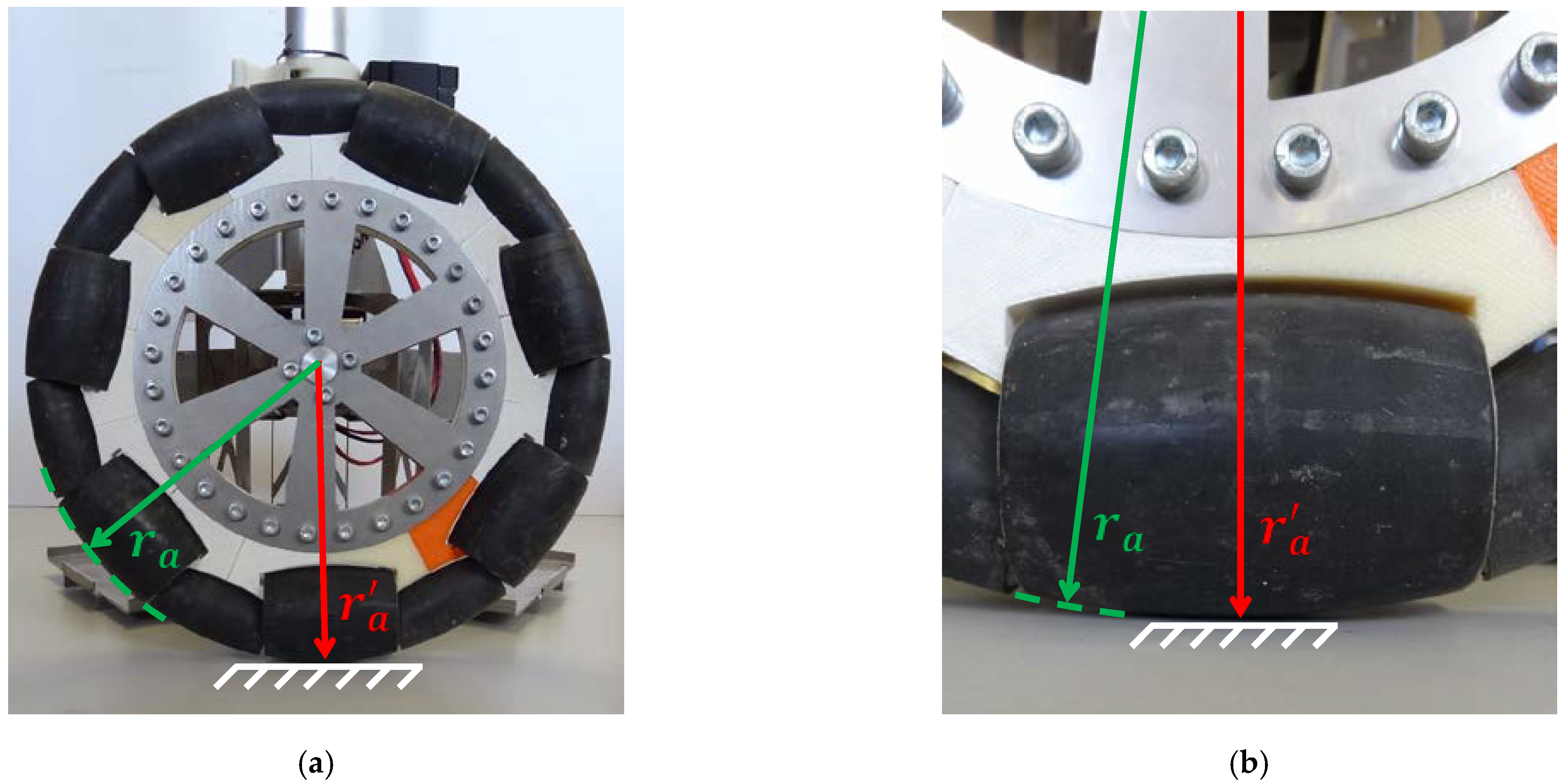
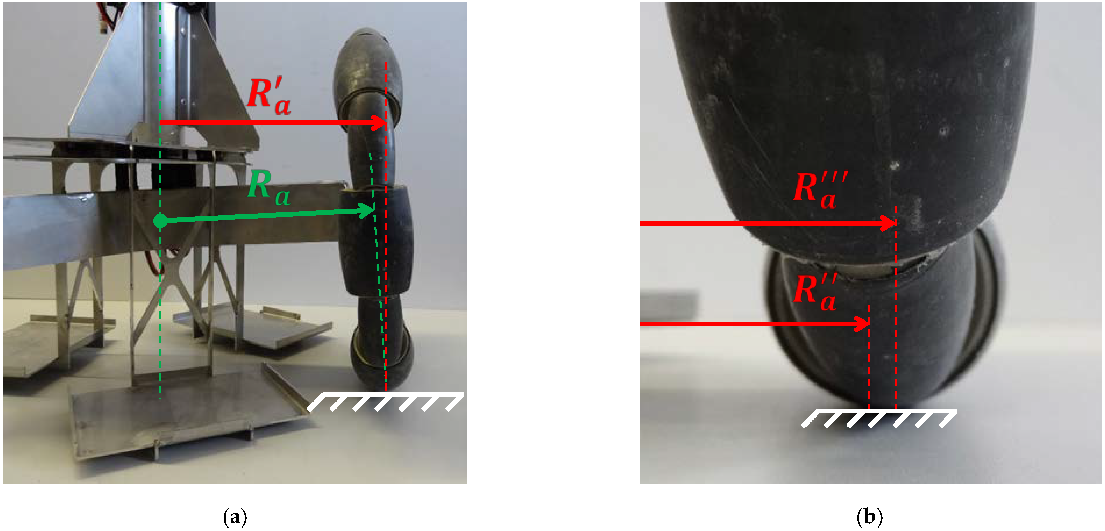
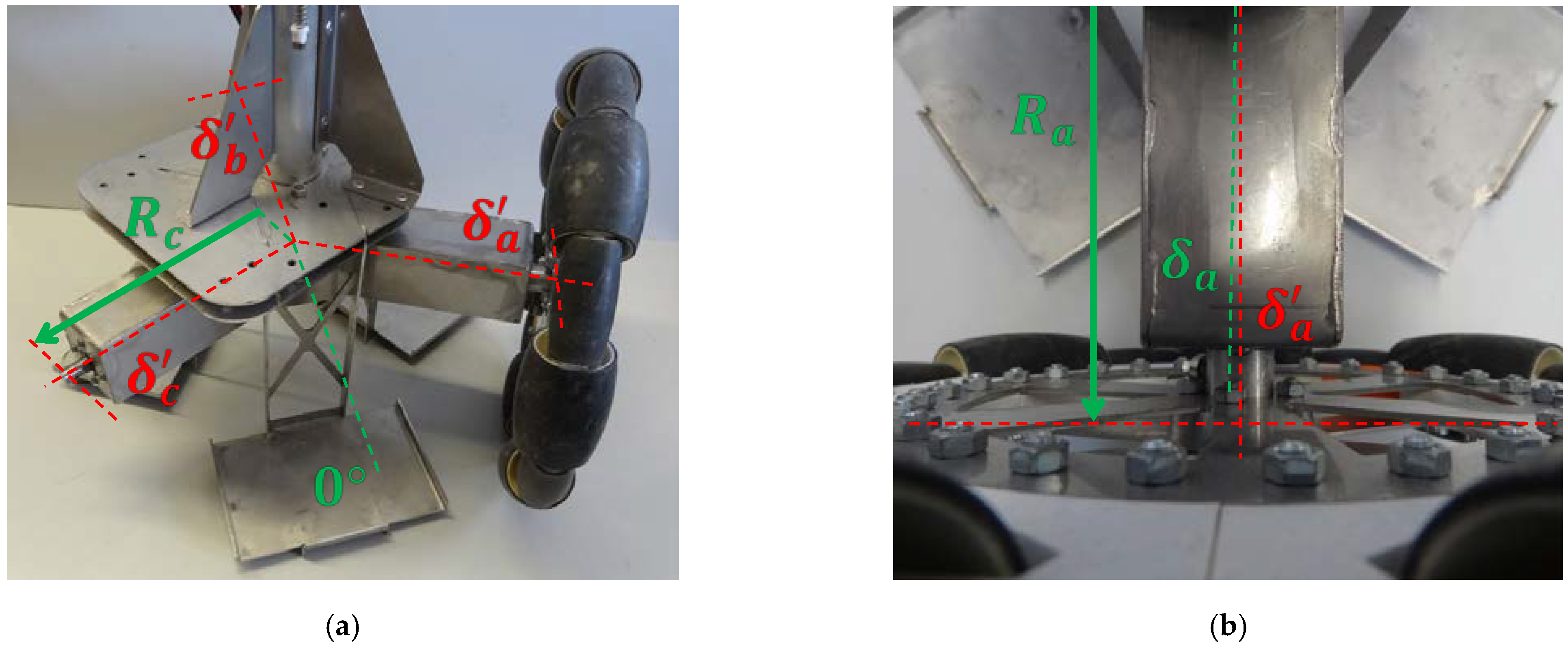
Table 5 compares the differences between the nominal and calibrated kinematic parameters obtained with STE-GA5. Unexpectedly, the differences between the nominal and calibrated values of the distance from the wheels to the center of the mobile robot ( R a , R b , R c ) are higher than 10%, likely caused by the bending of the structure that supports the wheels (wheelbase). The differences in the effective values of the radii of the wheels ( r a , r b , r c ) are in a range from 2 to 5%, probably caused by the complex assembly of the wheels. Finally, the values of the angular orientation of the wheels ( δ a , δ b , δ c ) vary within a very small range (0.18% and 0.52%), confirming the good alignment of the wheels and DC motors during the assembly of the mobile robot.
The exact value of the best inverse of the compact kinematic matrix M 1 computed from the effective value of the kinematic parameters obtained with STE-GA5 is:
M S T E G A 5 1 = [ 0.0892930568372762 0.0005606566978203 0.0867466159313470       0.0520955668635434 0.1010213675626970 0.0533117820461363       0.2364093797047320       0.2341358647406650 0.2353792947863630 ]
Finally, Table 6 summarizes the average RMS errors and average maximum errors obtained with the uncalibrated and calibrated kinematic parameters. These validation results have been obtained with the five repetitions of the 36 calibration trajectories registered for validation (180 validation experiments). 
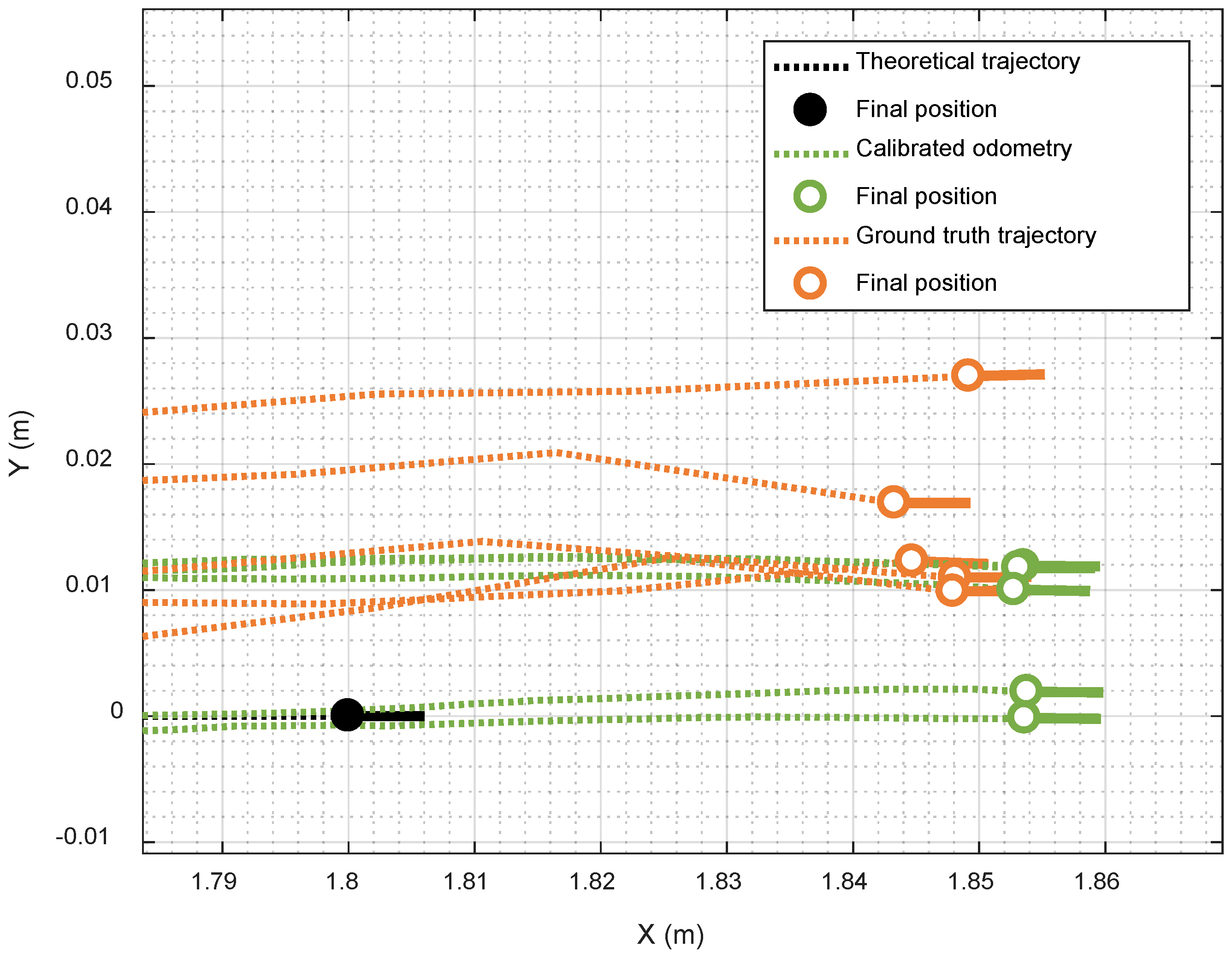
Table 6 shows that the improvement computed from the validation value of the cost function (82.1%) is representative of the trajectory improvements achieved. The application of the calibrated kinematic parameters showed an improvement of 67 % in the evaluation of the RMS error distance between the odometry trajectory and the ground truth trajectory, and an improvement of 71% in the RMS error evaluation of the absolute difference between the angular orientation of the mobile robot during these trajectories. The application of the calibrated kinematic parameters also showed a reduction in the maximum absolute differences between the odometry and ground truth trajectories, which have been reduced from 76 mm to 23 mm and from 5.86° to 1.77°. Similar improvements have been obtained in the error in the determination of the final location and angular orientation of the mobile robot that has been reduced from 74 mm to 16 mm and from and from 5.32° to 0.73°. 
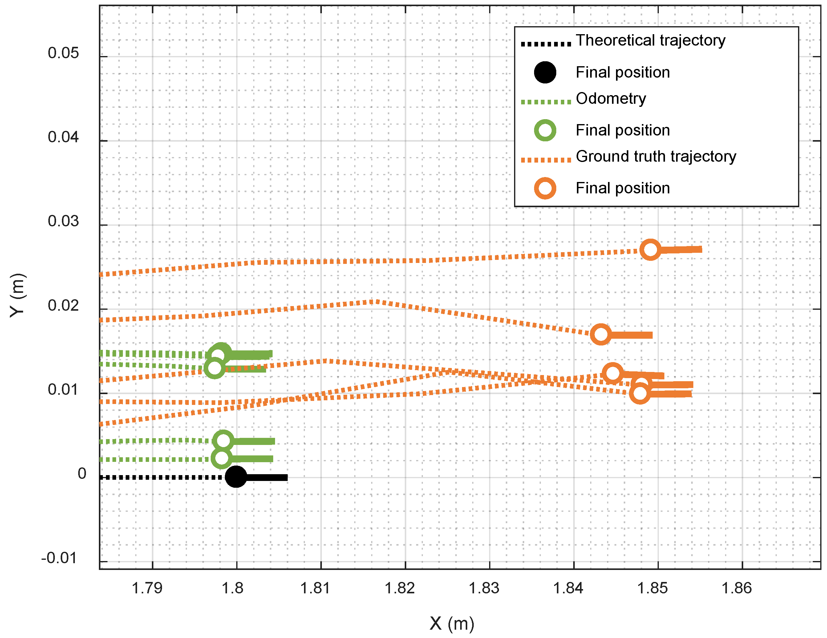
Figure 10 shows the application of the calibrated odometry to the trajectories shown previously in Figure 7, which correspond to five repetitions of the R1 calibration trajectory.

4. Discussion and Conclusions

This paper proposes a general procedure to evaluate and correct the systematic odometry errors of a real three-wheeled omnidirectional mobile robot (1.760 m, 30 Kg) designed as a versatile personal assistant tool. This procedure is based on the definition of 36 representative straight and curved calibration trajectories which together depict a characteristic flower-shaped figure.
The odometry and ground truth trajectories measured while performing each one of these calibration trajectories are measured and registered for later offline fitting of the kinematic parameters of the mobile robot in order to match these two trajectories. This paper has evaluated the use of different trajectory subsets and the use of two iterative matching strategies based on gradient search minimization and genetic algorithms. The best matching between odometry and ground truth trajectories has been obtained using genetic algorithms and five repetitions of all calibration trajectories. The fitting of the kinematic parameters has shown differences higher than 10% in the distance from the wheels to the center of the mobile robot ( R a , R b , R c ) , and between 2 and 5% in the radii of the wheels ( r a , r b , r c ) . This approach has the advantage of the feasible physical interpretation of the fitting results in the omnidirectional mobile robot.
The fitting results have been validated with five new additional repetitions of all these measured trajectories, providing an average improvement of 82% in the evaluation of the multivariable cost function that compares the final position and orientation of the mobile robot. The best performances of the genetic algorithm agree with the results of Savaee et al. [15], and confirm that the mutation and combinations generated during the search based on genetic algorithms has the best chance to detect the global minimum of the multivariate function that summarizes the differences between the odometry and ground truth trajectories of the mobile robot. In this case, the genetic algorithm search (strategy STE-GA5) required 187 iterations and 37.545 function counts to meet the stopping criteria.
The final conclusion of the comparative calibration analysis performed in this work is that the use of curved calibration trajectories is more representative to calibrate the kinematic parameters of an omnidirectional mobile robot. This conclusion agrees with Batlle et al. [17], who proposed the use of four curved trajectories for general omnidirectional mobile robot calibration, and with Maddahi et al. [11], who concluded that the performance of a calibration procedure depends on the type of trajectory analyzed.
Future works will analyze the application of this procedure to different units of the same mobile robot type in order to validate its application in a general manufacturing stage.

Author Contributions

Conceptualization, J.P.; Investigation, E.R. and E.C.; Methodology, J.P. and E.R.; Software, E.C.; Writing—original draft, E.R.; Writing—review & editing, J.P. All authors have read and agreed to the published version of the manuscript.

Funding

This research received no external funding.

Institutional Review Board Statement

Not applicable.

Informed Consent Statement

Not applicable.

Data Availability Statement

Not applicable.

Conflicts of Interest

The authors declare that they have no conflict of interest.

Appendix A

Table A1. Description of the motion commands and the corresponding target angular velocities of the wheels corresponding to the calibration trajectories shown in Figure 9.
TrajectoryMotion CommandTarget Angular Velocities (rpm)
v   ( m / s ) α ( ° ) ω ( r a d / s ) d ( m ) ω M a ω M b   ω M c  
R10.35001.0−19.5570.00019.557
R20.353001.0−11.291−11.29122.583
R30.356001.00.000−19.55719.557
R40.359001.011.291−22.58311.291
R50.3512001.019.557−19.5570.000
R60.3515001.022.583−11.291−11.291
R70.3518001.019.5570.000−19.557
R80.3521001.011.29111.291−22.583
R90.3524001.00.00019.557−19.557
R100.3527001.0−11.29122.583−11.291
R110.3530001.0−19.55719.5570.000
R120.3533001.0−22.58311.29111.291
G10.3500.351.0−15.1544.40423.961
G20.35300.351.0−6.888−6.88826.986
G30.35600.351.04.404−15.15423.961
G40.35900.351.015.695−18.17915.695
G50.351200.351.023.961−15.1544.404
G60.351500.351.026.986−6.888−6.888
G70.351800.351.023.9614.404−15.154
G80.352100.351.015.69515.695−18.179
G90.352400.351.04.40423.961−15.154
G100.352700.351.0−6.88826.986−6.888
G110.353000.351.0−15.15423.9614.404
G120.353300.351.0−18.17915.69515.695
B10.350−0.351.0−23.961−4.40415.154
B20.3530−0.351.0−15.695−15.69518.179
B30.3560−0.351.0−4.404−23.96115.154
B40.3590−0.351.06.888−26.9866.888
B50.35120−0.351.015.154−23.961−4.404
B60.35150−0.351.018.179−15.695−15.695
B70.35180−0.351.015.154−4.404−23.961
B80.35210−0.351.06.8886.888−26.986
B90.35240−0.351.0−4.40415.154−23.961
B100.35270−0.351.0−15.69518.179−15.695
B110.35300−0.351.0−23.96115.154−4.404
B120.35330−0.351.0−26.9866.8886.888

References

  1. Borenstein, J.; Koren, Y. Motion Control Analysis of a Mobile Robot. J. Dyn. Syst. Meas. Control 1987, 109, 73–79. [Google Scholar] [CrossRef] [Green Version]
  2. Borenstein, J.; Everett, H.R.; Feng, L.; Wehe, D. Mobile Robot Positioning: Sensors and Techniques. J. Robot. Syst. 1997, 14, 231–249. [Google Scholar] [CrossRef]
  3. Borenstein, J.; Feng, L. Measurement and correction of systematic odometry errors in mobile robots. IEEE Trans. Robot. Autom. 1996, 12, 869–880. [Google Scholar] [CrossRef] [Green Version]
  4. Gargiulo, A.M.; di Stefano, I.; Genova, A. Model-Based Slippage Estimation to Enhance Planetary Rover Localization with Wheel Odometry. Appl. Sci. 2021, 11, 5490. [Google Scholar] [CrossRef]
  5. Zwierzchowski, J.; Pietrala, D.; Napieralski, J.; Napieralski, A. A Mobile Robot Position Adjustment as a Fusion of Vision System and Wheels Odometry in Autonomous Track Driving. Appl. Sci. 2021, 11, 4496. [Google Scholar] [CrossRef]
  6. Xue, H.; Fu, H.; Dai, B. IMU-Aided High-Frequency Lidar Odometry for Autonomous Driving. Appl. Sci. 2019, 9, 1506. [Google Scholar] [CrossRef] [Green Version]
  7. Palacín, J.; Martínez, D.; Rubies, E.; Clotet, E. Mobile Robot Self-Localization with 2D Push-Broom LIDAR in a 2D Map. Sensors 2020, 20, 2500. [Google Scholar] [CrossRef] [PubMed]
  8. Lluvia, I.; Lazkano, E.; Ansuategi, A. Active Mapping and Robot Exploration: A Survey. Sensors 2021, 21, 2445. [Google Scholar] [CrossRef] [PubMed]
  9. Xiao, K.; Yu, W.; Liu, W.; Qu, F.; Ma, Z. High-Precision SLAM Based on the Tight Coupling of Dual Lidar Inertial Odometry for Multi-Scene Applications. Appl. Sci. 2022, 12, 939. [Google Scholar] [CrossRef]
  10. Sousa, R.B.; Petry, M.R.; Moreira, A.P. Evolution of Odometry Calibration Methods for Ground Mobile Robots. In Proceedings of the IEEE International Conference on Autonomous Robot Systems and Competitions (ICARSC), Ponta Delgada, Portugal, 15–17 April 2020; pp. 294–299. [Google Scholar] [CrossRef]
  11. Maddahi, Y.; Maddahi, A.; Sepehri, N. Calibration of omnidirectional wheeled mobile robots: Method and experiments. Robotica 2013, 31, 969–980. [Google Scholar] [CrossRef]
  12. Lin, P.; Liu, D.; Yang, D.; Zou, Q.; Du, Y.; Cong, M. Calibration for Odometry of Omnidirectional Mobile Robots Based on Kinematic Correction. In Proceedings of the 14th International Conference on Computer Science & Education (ICCSE), Toronto, ON, Canada, 19–21 August 2019; pp. 139–144. [Google Scholar] [CrossRef]
  13. Li, Y.; Ge, S.; Dai, S.; Zhao, L.; Yan, X.; Zheng, Y.; Shi, Y. Kinematic Modeling of a Combined System of Multiple Mecanum-Wheeled Robots with Velocity Compensation. Sensors 2020, 20, 75. [Google Scholar] [CrossRef] [Green Version]
  14. Lu, Z.; He, G.; Wang, R.; Wang, S.; Zhang, Y.; Liu, C.; Chen, D.; Hou, T. An Orthogonal Wheel Odometer for Positioning in a Relative Coordinate System on a Floating Ground. Appl. Sci. 2021, 11, 11340. [Google Scholar] [CrossRef]
  15. Savaee, E.; Hanzaki, A.R. A New Algorithm for Calibration of an Omni-Directional Wheeled Mobile Robot Based on Effective Kinematic Parameters Estimation. J. Intell. Robot. Syst. 2021, 101, 28. [Google Scholar] [CrossRef]
  16. Bożek, A. Discovering Stick-Slip-Resistant Servo Control Algorithm Using Genetic Programming. Sensors 2022, 22, 383. [Google Scholar] [CrossRef] [PubMed]
  17. Batlle, J.A.; Font-Llagunes, J.M.; Barjau, A. Calibration for mobile robots with an invariant Jacobian. Robot. Auton. Syst. 2010, 58, 10–15. [Google Scholar] [CrossRef]
  18. Palacín, J.; Clotet, E.; Martínez, D.; Martínez, D.; Moreno, J. Extending the Application of an Assistant Personal Robot as a Walk-Helper Tool. Robotics 2019, 8, 27. [Google Scholar] [CrossRef] [Green Version]
  19. Penteridis, L.; D'Onofrio, G.; Sancarlo, D.; Giuliani, F.; Ricciardi, F.; Cavallo, F.; Greco, A.; Trochidis, I.; Gkiokas, A. Robotic and Sensor Technologies for Mobility in Older People. Rejuvenation Res. 2017, 20, 401–410. [Google Scholar] [CrossRef] [PubMed] [Green Version]
  20. Palacín, J.; Rubies, E.; Clotet, E.; Martínez, D. Evaluation of the Path-Tracking Accuracy of a Three-Wheeled Omnidirectional Mobile Robot Designed as a Personal Assistant. Sensors 2021, 21, 7216. [Google Scholar] [CrossRef] [PubMed]
  21. Palacín, J.; Martínez, D.; Rubies, E.; Clotet, E. Suboptimal Omnidirectional Wheel Design and Implementation. Sensors 2021, 21, 865. [Google Scholar] [CrossRef] [PubMed]
  22. Palacín, J.; Martínez, D. Improving the Angular Velocity Measured with a Low-Cost Magnetic Rotary Encoder Attached to a Brushed DC Motor by Compensating Magnet and Hall-Effect Sensor Misalignments. Sensors 2021, 21, 4763. [Google Scholar] [CrossRef]
  23. Crowley, J.L. Asynchronous Control of Orientation and Displacement in a Robot Vehicle. In Proceedings of the 1989 IEEE International Conference on Robotics and Automation, Scottsdale, AZ, USA, 14–19 May 1989; pp. 1277–1282. [Google Scholar] [CrossRef]
  24. Feng, L.; Koren, Y.; Borenstein, J. Cross-Coupling Motion Controller for Mobile Robots. IEEE J. Control. Syst. 1993, 13, 35–43. [Google Scholar] [CrossRef]
  25. Goldberg, D. What every computer scientist should know about floating-point arithmetic. ACM Comput. Surv. 1991, 23, 5–48. [Google Scholar] [CrossRef]
  26. Smieszek, M.; Dobrzanska, M.; Dobrzanski, P. Measurement of Wheel Radius in an Automated Guided Vehicle. Appl. Sci. 2020, 10, 5490. [Google Scholar] [CrossRef]
  27. Hess, D.; Kuenemund, F.; Roehrig, C. Simultaneous Calibration of Odometry and external Sensors of Omnidirectional Automated Guided Vehicles (AGVs). In Proceedings of the 47st International Symposium on Robotics, Munich, Germany, 21–22 June 2016; pp. 1–8. [Google Scholar]
  28. Yagfarov, R.; Ivanou, M.; Afanasyev, I. Map Comparison of Lidar-based 2D SLAM Algorithms Using Precise Ground Truth. In Proceedings of the 15th International Conference on Control, Automation, Robotics and Vision (ICARCV), Singapore, 18–21 November 2018; pp. 1979–1983. [Google Scholar] [CrossRef]
  29. Iaboni, C.; Patel, H.; Lobo, D.; Choi, J.W.; Abichandani, P. Event Camera Based Real-Time Detection and Tracking of Indoor Ground Robots. IEEE Access 2021, 9, 166588–166602. [Google Scholar] [CrossRef]
Figure 1. Mobile robot APR-02: (a) general view of the mobile robot and (b) detail of its omnidirectional motion system.
Applsci 12 02606 g001
Figure 2. Parametric definition of the omnidirectional motion system of the mobile robot APR-02: (a) general representation of the three omnidirectional wheels and (b) detail of the parameters of one omnidirectional wheel. ( X R , Y R ) represents the mobile robot frame in which X R is the front of the mobile robot.
Applsci 12 02606 g002
Figure 3. General view (a) and detail (b) of the wheel radius and the point of contact of the wheel with the floor: r a depicts the nominal radius (green font and lines) and r a the real or effective radius (red font and lines).
Applsci 12 02606 g003
Figure 4. General view (a) and detail (b) of the point of contact with the floor and the distance from the wheel to the center of the mobile robot: R a depicts the nominal or design value (green font and lines) and R a the real or effective value (representing R a as the average value of R a and R a , red font and lines).
Applsci 12 02606 g004
Figure 5. General view (a) and detail (b) of the angular orientation of the front-left wheel (wheel a) relative to the mobile robot frame: δ a depicts the nominal or design value (green font and lines) and δ a is the real or effective value (red font and lines).
Applsci 12 02606 g005
Figure 6. Representation of the ground truth trajectory of the mobile robot (orange line) and the trajectory estimated with the odometry (green line): (a) complete trajectories; (b) angle and distance differences between the trajectory positions estimated with the odometry and the SLAM procedure.
Applsci 12 02606 g006
Figure 7. Planned trajectory (back dotted line) zoomed at the planned ending position and orientation of the mobile robot (black point and line); measured ground truth trajectories (orange dotted line) detailing the final position and orientation of the mobile robot (orange circle and line); and measured odometry trajectory (green dotted line) detailing the ending position and orientation of the mobile robot (green circle and line).
Applsci 12 02606 g007
Figure 8. Flowchart of the complete calibration procedure.
Applsci 12 02606 g008
Figure 9. Representation of the ideal flower-shaped trajectories proposed to calibrate the odometry of the omnidirectional mobile robot APR-02.
Applsci 12 02606 g009
Figure 10. Planned trajectory (back dotted line) zoomed at the planned ending position and orientation of the mobile robot (black point and line); measured ground truth trajectories (orange dotted line) detailing the final position and orientation of the mobile robot (orange circle and line); and odometry trajectories measured after calibration (green dotted line) detailing the ending position and orientation of the mobile robot (green circle and line).
Applsci 12 02606 g010
Table 1. Sensitivity of M 1 to the values of the nominal kinematic parameters of the wheel a.
Δ M 1 Δ R a | R a = 0.195   m Δ M 1 Δ r a | r a = 0.148   m Δ M 1 Δ δ a | δ a = 60 °
[         0.1461         0.1461         0.1461 0.0843 0.0843 0.0843 0.4325 0.4325 0.4325 ] [ 0.5774 0.0000 0.0000       0.3333 0.0000 0.0000       1.7094 0.0000 0.0000 ] [ 0.0000         0.0493 0.0493 0.0000 0.0285       0.0285 0.0000 0.1461       0.1461 ]
Table 2. Sensitivity of M 1 to the values of the nominal kinematic parameters of the wheel b.
Δ M 1 Δ R b | R b = 0.195   m Δ M 1 Δ r b | r b = 0.148   m Δ M 1 Δ δ b | δ b = 180 °
[         0.0000         0.0000         0.0000         0.1687         0.1687         0.1687 0.4325 0.4325 0.4325 ] [ 0.0000             0.0000 0.0000 0.0000 0.6667 0.0000 0.0000   1.7094 0.0000 ] [         0.0000 0.0000       0.0000 0.0570 0.0000       0.0570       0.1461 0.0000 0.1461 ]
Table 3. Sensitivity of M 1 to the values of the nominal kinematic parameters of the wheel c.
Δ M 1 Δ R c | R c = 0.195   m Δ M 1 Δ r c | r c = 0.148   m Δ M 1 Δ δ c | δ c = 300 °
[ 0.1461 0.1461 0.1461 0.0843 0.0843 0.0843 0.4325 0.4325 0.4325 ] [ 0.0000 0.0000 0.5774 0.0000 0.0000 0.3333 0.0000 0.0000 1.7094 ] [ 0.0493 0.0493 0.0000 0.0285 0.0285 0.0000 0.1461 0.1461 0.0000 ]
Table 4. Trajectories, calibration strategies and results obtained.
TrajectoriesStrategyMethod M 1 C F C A L I B R A T I O N C F V A L I D A T I O N Improvement
Applsci 12 02606 i001AllNone- [ 0.0854 0.0000 0.0854       0.0493 0.0987 0.0493 0.2530       0.2530 0.2530 ] -0.1242-
Applsci 12 02606 i002
R1, R5, R9
STAGA1 [ 0.0866       0.0015 0.0891       0.0517 0.1012 0.0536       0.2567       0.2552 0.2539 ] 0.02140.12152.18%
Fmin1 [ 0.0881       0.0009 0.0876       0.0497 0.1024 0.0517       0.2594       0.2588 0.2565 ] 0.02280.1386−11.61%
GA5 [ 0.0849       0.0043 0.0909       0.0503 0.1014 0.0507       0.2559       0.2560 0.2561 ] 0.02020.1267−2.03%
Fmin5 [ 0.0883       0.0007 0.0874       0.0505 0.1015 0.0509       0.2569       0.2593 0.2598 ] 0.01920.1436−15.62%
Applsci 12 02606 i003
B2, B6, B10, G12, G4, G8
STBGA1 [ 0.0898 0.0010 0.0851       0.0533 0.1000 0.0567       0.2379       0.2340 0.2335 ] 0.01700.033373.19%
Fmin1 [ 0.0862 0.0009 0.0835       0.0479 0.0964 0.0496       0.2404       0.2352 0.2369 ] 0.05030.069144.36%
GA5 [ 0.0894 0.0011 0.0860       0.0525 0.0999 0.0539       0.2369       0.2340 0.2350 ]   0.01660.023281.36%
Fmin5 [ 0.0857       0.0003 0.0844       0.0477 0.0966 0.0486       0.2393       0.2356 0.2376 ] 0.05250.067745.52%
Applsci 12 02606 i004
R1…R12
STCGA1 [ 0.0907 0.0030 0.0844       0.0512 0.1014 0.0520       0.2579       0.2559 0.2567 ] 0.02640.1278−2.92%
Fmin1 [ 0.0883 0.0005 0.0871       0.0515 0.1014 0.0524       0.2494       0.2472 0.2479 ] 0.02580.081734.2 %
GA5 [ 0.0861       0.0018 0.0891       0.0511 0.1015 0.0523       0.2585       0.2565 0.2573 ] 0.02730.1308−5.31%
Fmin5 [ 0.0881 0.0001 0.0873       0.0512 0.1015 0.0524       0.2497       0.2475 0.2483 ] 0.02640.083233.00%
Applsci 12 02606 i005
B1…B12, G1…G12
STDGA1 [ 0.0897 0.0002 0.0864       0.0524 0.1001 0.0530       0.2373       0.2346 0.2364 ] 0.01990.024880.05%
Fmin1 [ 0.0852       0.0009 0.0844       0.0490 0.0968 0.0492       0.2398       0.2361 0.2383 ] 0.05390.066046.89%
GA5 [ 0.0892 0.0004 0.0874       0.0518 0.1027 0.0533       0.2365       0.2333 0.2358 ] 0.02020.026178.98%
Fmin5 [ 0.0851       0.0009 0.0845       0.0489 0.0967 0.0490       0.2393       0.2358 0.2383 ] 0.05540.066546.43%
Applsci 12 02606 i006
All
STEGA1 [ 0.0895 0.0007 0.0867       0.0528 0.1002 0.0537       0.2367       0.2346 0.2355 ] 0.02120.022681.83%
Fmin1 [ 0.0859       0.0008 0.0851       0.0497 0.0983 0.0501       0.2421       0.2397 0.2408 ] 0.05910.063648.82%
GA5 [ 0.0893 0.0006 0.0867       0.0521 0.1010 0.0533       0.2364       0.2341 0.2354 ] 0.02210.022282.14%
Fmin5 [ 0.0859       0.0007 0.0850       0.0495 0.0982 0.0501       0.2418       0.2394 0.2406 ] 0.06030.063448.97%
Table 5. Nominal and calibrated kinematic parameters (strategy STE-GA5) of the mobile robot.
R a   ( m ) R b   ( m ) R c   ( m ) r a   ( m ) r b   ( m ) r c   ( m ) δ a   ( ° ) δ b   ( ° ) δ c   ( ° )
Nominal0.1950.1950.1950.1480.1480.14860.0180.0300.0
Calibrated0.2186430.2157350.2162870.1550680.1515340.15272859.7397179.6820301.5735
Difference12.13%10.63%10.92%4.78%2.39%3.19%−0.43%−0.18%0.52%
Table 6. Summary of the average trajectory errors obtained with the uncalibrated and calibrated kinematic parameters.
RMS ErrorMax ErrorFinal position error C F V A L I D A T I O N
Distance
(m)
Abs(angle)
(°)
Distance
(m)
Abs(angle)
(°)
Distance
(m)
Abs(angle)
(°)
Uncalibrated0.0403.000.0765.860.0745.320.1242
Calibrated (STE-GA5)0.0130.860.0231.770.0160.730.0222
Improvement 67.00%71.22%68.99%69.82%78.38%86.24%82.14%
Publisher’s Note: MDPI stays neutral with regard to jurisdictional claims in published maps and institutional affiliations.

