One-Dimensional Convolutional Neural Network for Pipe Jacking EPB TBM Cutter Wear Prediction

Abstract

An earth pressure balance (EPB) TBM is used in soft ground conditions, and these conditions lead to the fluctuation and instability of machine parameters. Machine parameters influence cutter wear and tunnel excavation. For this reason, to evaluate and predict the cutter wear of an EPB TBM, a 1D CNN model was used to provide machine-parameter-based cutter wear prediction using an EPB TBM operational dataset. The machine parameters were split into 80% training and 20% test datasets. Compared to traditional machine learning applications and two deep neural network models, the proposed model provided reliable results with a reasonable computational time. The correlation coefficient was 89.6% $R^2$, the mean squared error (MSE) was 57.6, the mean absolute error (MAE) was 1.6, and the computational wall time was 3 min 22 s.

1. Introduction

A tunnel boring machine (TBM) is a mechanized tunnelling tool that excavates a wide range of geological formations. Unlike conventional tunnelling, mechanized tunnelling is widely preferred in the industry due to the safety, speed, and versatility of tunnel boring machines. However, TBMs encounter different adverse effects such as rock burst, clogging, groundwater, and cutter tool wear [1,2,3,4]. These events lead to time-consuming tunnel construction and high operational and maintenance costs for the tools. Furthermore, the failure of the cutting tool dominates the downtime and high maintenance cost in mechanized tunnelling [5,6,7]. Rong, Xuening, et al. [8] stated that unproper tool wear inspection leads to cutter head damage while the machine excavates a tunnel. According to Su Weilin et al. [9], if overworn cutters are not changed in time, higher torque occurs, and other parts of the TBM are damaged, resulting in excessive delay in the excavation process. Therefore, cutter wear prediction is crucial in the mechanized tunnelling industry. Several models have been provided by many researchers. They are classified as empirical, probabilistic, and artificial intelligence models.

2. Literature Review

Empirical and semiempirical models have been provided by previous authors [10,11,12,13,14,15,16,17,18] to predict the cutter wear of TBMs. They consider rock parameters (CAI, UCS, quartz content, Vicker’s hardness number (VHNR), fracturing degree, porosity, drilling rate index, and rock mass classification), machine properties (thrust, torque, penetration rate, rpm, and TBM diameter), and cutter geometry to estimate cutter tool life. However, they have drawbacks, such as requiring special laboratory equipment, working with a small number of input parameters, and having a high computational time due to the experimental setup process. However, Farrokh [19] provided a probabilistic approach using a regression-based empirical formula for tool life prediction. Moreover, they applied various multivariate regression analyses with geotechnical parameters (quartz content (EQC), soil strength (Tc), 60% passing soil size (D60), and standard penetration test (SPT)) for tool life estimation. Nevertheless, multivariable regression analysis is limited by the size of the input parameters. The probabilistic approach is not able to work with high-dimensional datasets. However, a TBM produces a large amount of data during excavation; thus, traditional regression analysis is not adequate for mechanized tunnelling evaluation. Therefore, many studies have been carried out to overcome the gap in the empirical formula and in the probabilistic models using artificial intelligence approaches. Most of the previous authors implemented artificial intelligence models for TBM penetration rate prediction [20,21,22,23,24,25,26,27,28,29,30,31,32,33]. Besides penetration rate prediction, artificial intelligence is rarely used for cutter wear prediction.

Arsalan M. et al. [34] established traditional machine learning models, such as Gaussian process regression, support vector regression, decision tree, and k-nearest neighbor, for cutter tool life prediction. In these applications, specific energy, quartz content, excavation depth, thrust force, cutter head rotation speed, penetration rate, screw rate, grouting pressure, and soil pressure were taken into account as the input, while disc cutter life (${\mathrm{m}}^3/\mathrm{cutter}$) was the output. However, these artificial intelligence models have disadvantages, such as overfitting, not being able to work with a large dataset, and memorizing the computational process. Massalov et al. [35] used the Norwegian University of Science and Technology (NTNU) cutter life index for cutter prediction. Rock mechanical properties (UCS, BTS, brittleness, and density) were used with an artificial neural network (ANN) and fuzzy logic algorithm. However, the NTNU-based model requires a specific laboratory setup to acquire cutter wear index. For this reason, Honggan Yu et al. [36] provided a 1D CNN model for disc cutter life prediction and considered the operational parameters of a TBM. The proposed model is related to the new health index for real-time estimation based on the small rolling excavated distance and maximal rolling distance. Nevertheless, according to Honggan Yu et al. [36], the proposed model had a shortcoming due to the disc cutters hardly reaching their wear limit for applications of the health index. Furthermore, the model requires the real maximal rolling distance, and if the real maximal rolling distance is not adequate, an alternative rolling distance should be created. Therefore, the model is complicated and not easy to implement. However, K. Elbaz et al. [37] implemented the group method handling–genetic algorithm combination, with geological parameters and operational properties (UCS, Qc, RQD, PR, TH, GP, SP, and SE) as the input and Hf (${\mathrm{m}}^3/\mathrm{cutter}$) utilized as the output for the estimation model. The GMDH is a self-organizing method that can be applied to solve complex problems on nonlinear systems, despite it having drawbacks, such as being trapped in a local minimum and being unable to find a global minimum.

In summary, most of the previous models have been applied to hard rock TBM operations, and they have several shortcomings. For this reason, a new 1D CNN model is proposed in this research. Unlike prior applications, the proposed model is created for soft ground mechanized tunnelling and big data. The input parameters were obtained from a micro-tunnelling project rather than large-scale TBM sizes. The proposed model provides a more reliable and fast computation compared to previous models.

The main purpose of this research is to investigate pipe jacking EPB TBM cutter tool life prediction using the suited 1D CNN regression through high-dimensional machine parameters and to overcome the gaps in the previous model. During the shield-type tunnel construction of a water tunnel in Japan, a huge number of real-time operational data were recorded. In this research, actual tool wear (wear amount in mm) was recorded from inspection points 205, 344, 493, and 623, and machine parameters were collected from a total of 723 rings in the shield tunnel. Moreover, the main geology of the tunnel is sandy silt and sandy gravel. Additionally, the novel 1D CNN regressor model was originally made for soft ground mechanized tunnelling. The model was compared to different traditional machine learning models and deep neural networks (extratree regression, light gradient boosting, gradient boosting, random forest, AdaBoost, k-NN regression, multilayer perceptron neural network, and LSTM) to determine the model’s high reliability. The main contribution of this research is that the algorithm works with soft ground mechanized tunnelling operational parameters. It provides a low computational time, which is 3 min 22 s, and it can work with high-dimensional datasets. Compared to limited site investigation information, the algorithm can work with real-time recorded machine parameters. Figure 1 shows the proposed 1D CNN disc cutter wear prediction using the information of the inspection points of the tunnel and the EPB TBM operational data. The inspection points’ information was used to obtain the cutter wear index for the output data, and the operational data were used as the input features.

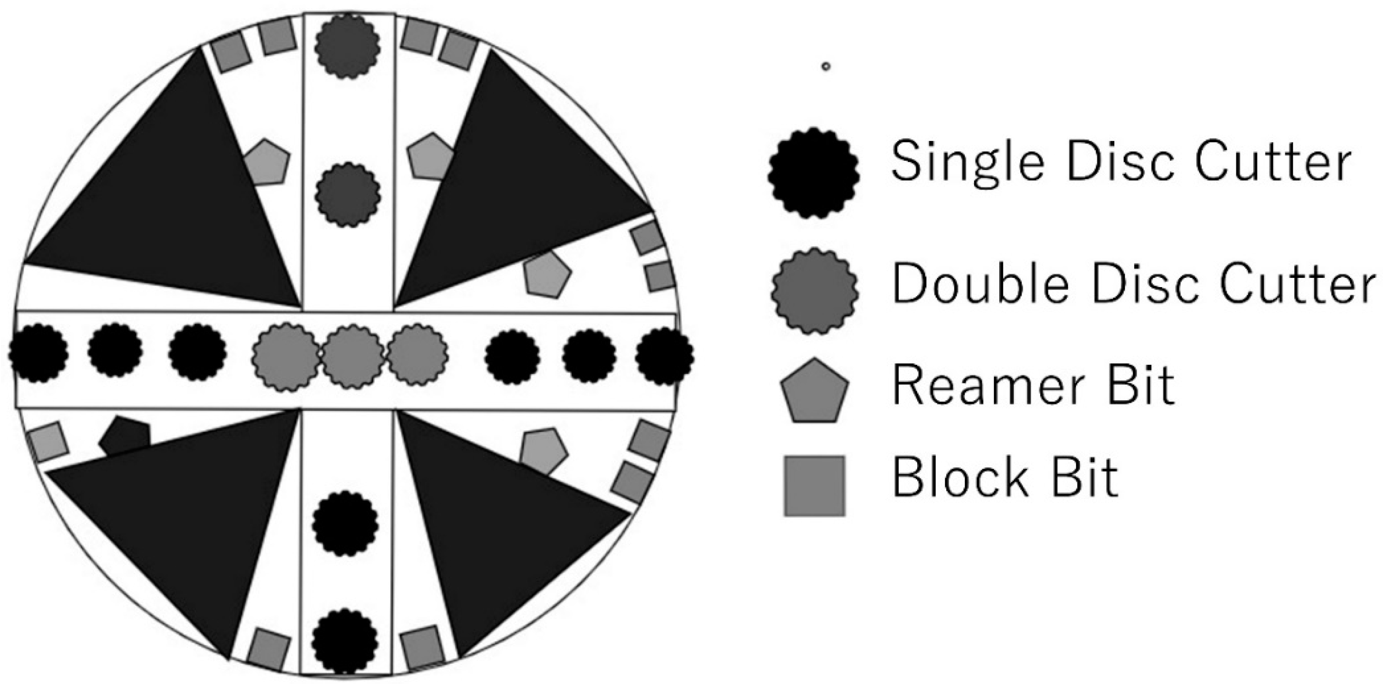
3. EPB Machine Specifications

The water tunnel project is an agricultural water transport tunnel project, and a pipe-jacking-type EPB TBM was operated in the tunnel excavation. A picture of the cutter arrangement is shown in Figure 2. The machine specifications are shown in

Table 1. EPB TBM machine specifications.

Machine Specifications
Shield outer diameter (m)	3.12
Shield length (m)	7.42
Thrust force (kN/m2)	1342
Shield jack speed (mm/min)	63
Torque (kN.m)	886

. The tunnel diameter is 2.95 m. The daily tunnel advancement is between 2 and 8 m.

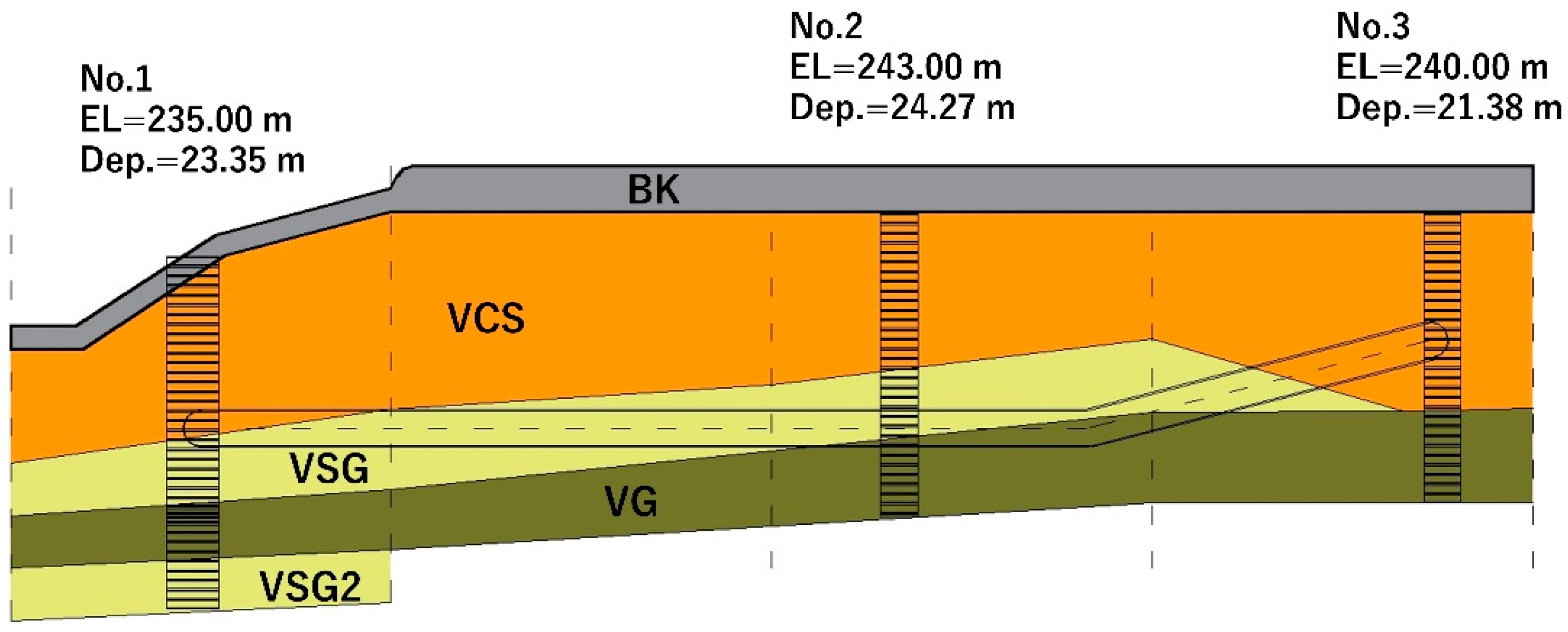
4. Engineering Geology

The water tunnel geology was identified by three main boreholes in a site investigation. Borehole 1 is the entrance shaft, and its length is 23.35 m; borehole 2 is the middle of the tunnel, with a 24.27 m length; and borehole 3 is the reaching shaft, with a length of 21.38 m. Figure 3a shows the borehole 1 core sampling, which consisted of silty clay and silt mixed gravel. Figure 3b presents the soil type of the middle shaft (borehole 2), which consisted of sandy clay and silty sand. Figure 3c shows the reaching shaft (borehole 3) soil type, which consisted of clay silt and silty gravel. Figure 4 illustrates the borehole locations and tunnel lithologies on the engineering geology map. Moreover,

Table 2. Description of lithologies.

Borehole Number	Depth (m)	Soil Layers	Soil Layers	Test Points	Elastic Module (MN/m2)	Consolidated Undrained Triaxial Test
						Cohesion $(\mathbf{kN}/{\mathbf{m}}^2)$	Friction Angle
No. 1	7.50	Silty clay	Vcs	6	15.97	16.4	31.04
	10	Sandy silt mixed with gravel	Vcs	5	14.76	21.4	41.37
No. 2	16	Sandy clay	Vsg	50	83.45	92.1	31.27
	19.50	Silty sand	Vsg	18	45.20	60.5	23.33
No. 3	11	Silty clay	Vcs	4	4.37	19.7	27.25
	14.50	Silty gravel	Vg	34	62.37	2.7	40.44

presents the soil layer classes and consolidated undrained triaxial test results.

In this study, soil layers were divided into three main groups on the basis of grain size distribution. Section 4.1 explains the grain size distribution and characterization in detail.

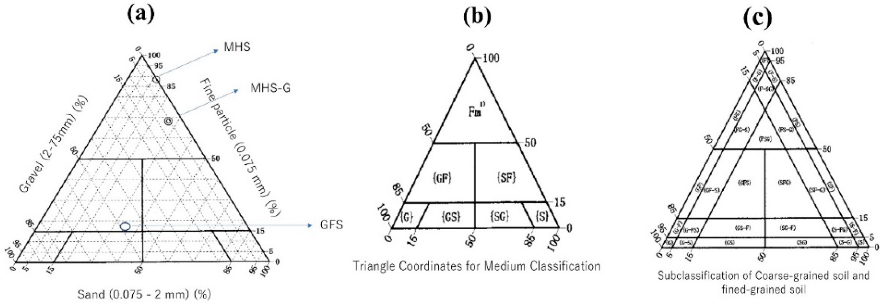
4.1. Grain Size Distribution and Characteristics

The granular characteristics and soil classification are based on the Japan Unified Soil Classification System [38,39,40]. The system is correlated with the World Reference Base for Soil Resources and Soil Taxonomy USDA. The Vcs layer is classified as high silt content and gravel–mixed silty sand content (MH and MHS-G). The Vsg layer is identified as two different soil types, (1) fine-grained sandy gravel and (2) high gravel content with GFS and MHS. The Vg layer is described as fine-grained, pulverized sand and refers to GFS with a large amount of gravel. The particle size characteristics are divided into the following four groups: gravel (2 mm or more), sand ($75 \mathsf{\mu }$m to 2 mm), silt (5 to $75 \mathsf{\mu }$m), and clay (5 $\mathsf{\mu }$m or less). The soil properties accumulate into the following three main groups: sandy soil, gravel soil, and cohesive soil. The granular system is dependent on the triangular system [40], which is shown in Figure 5a. The triangular coordinates for the medium classification are illustrated in Figure 5b. The subclassification of coarse soil and fine-grained soil is presented in Figure 5c.

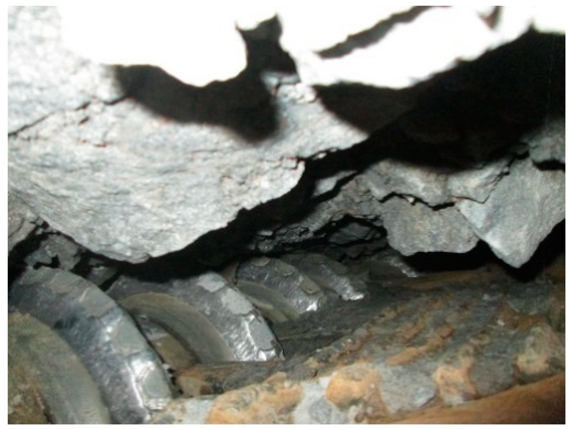
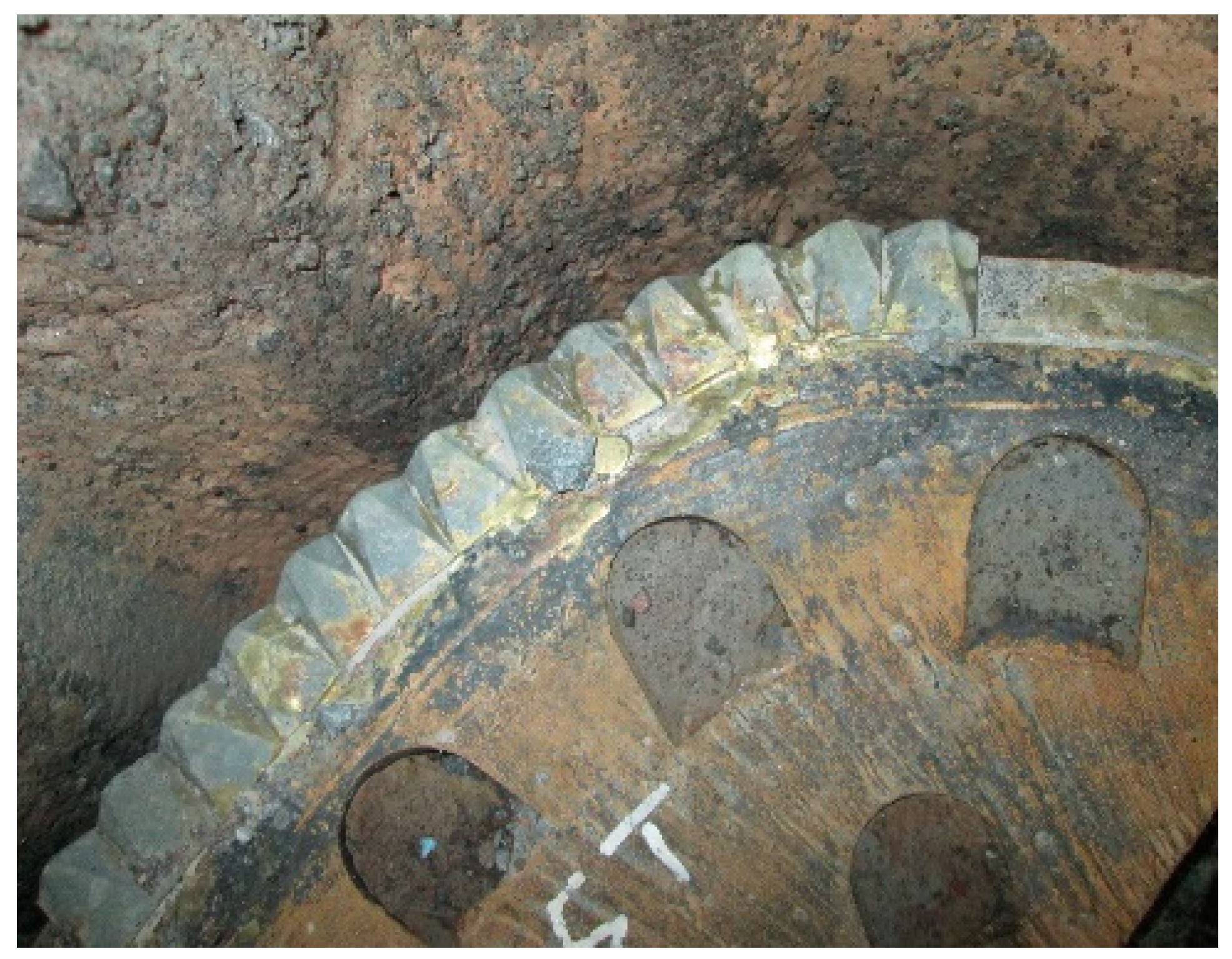
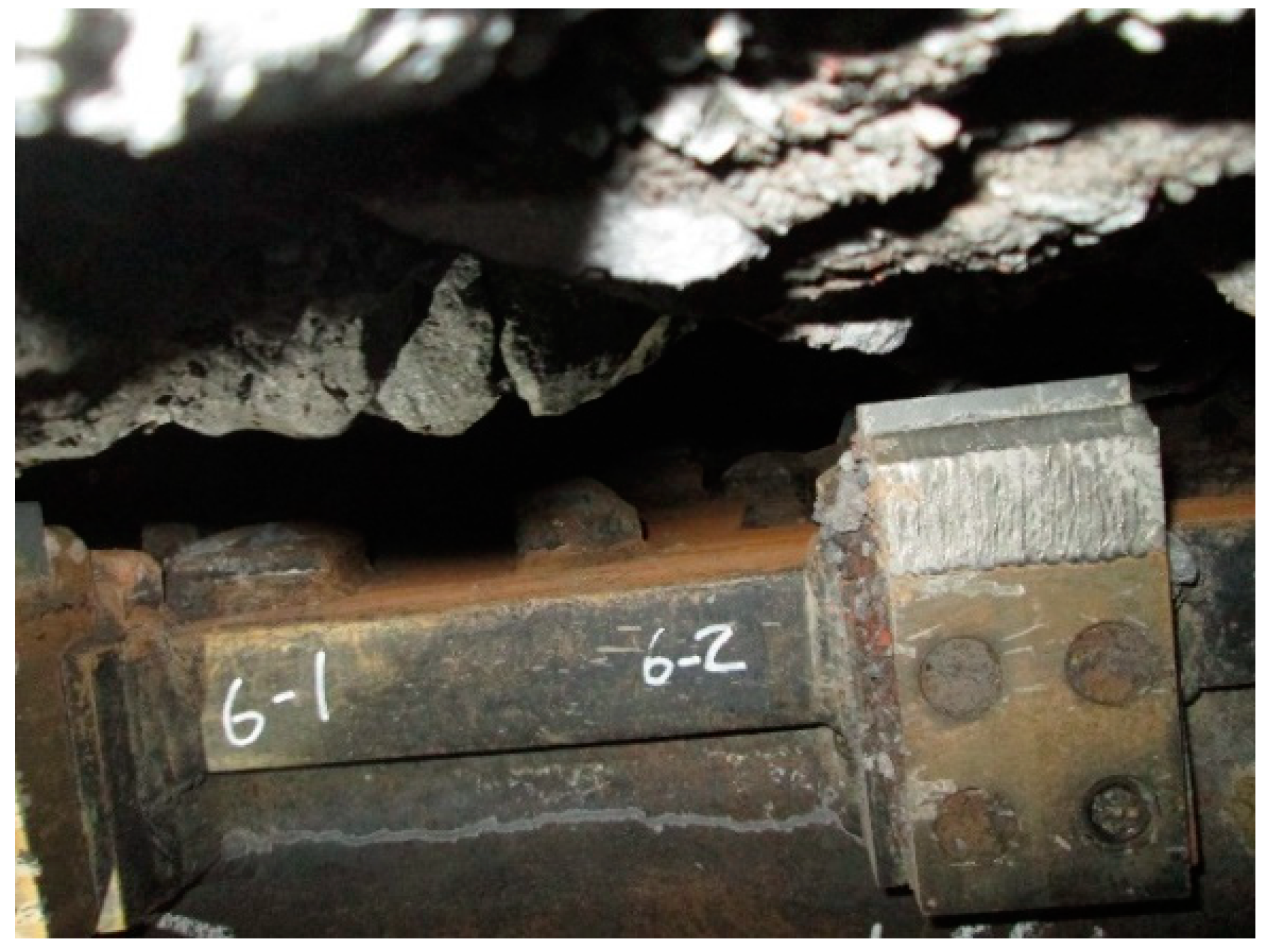
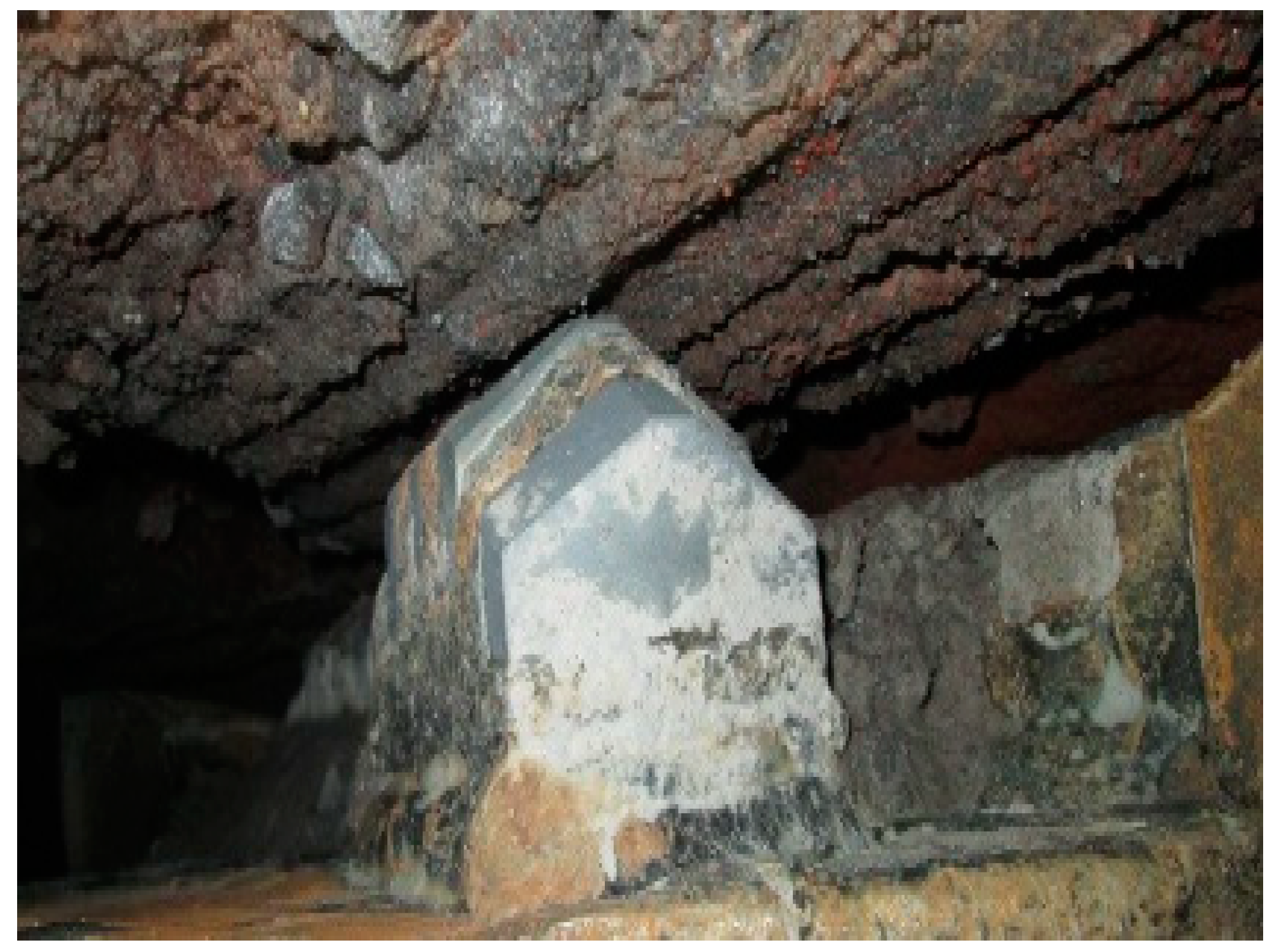
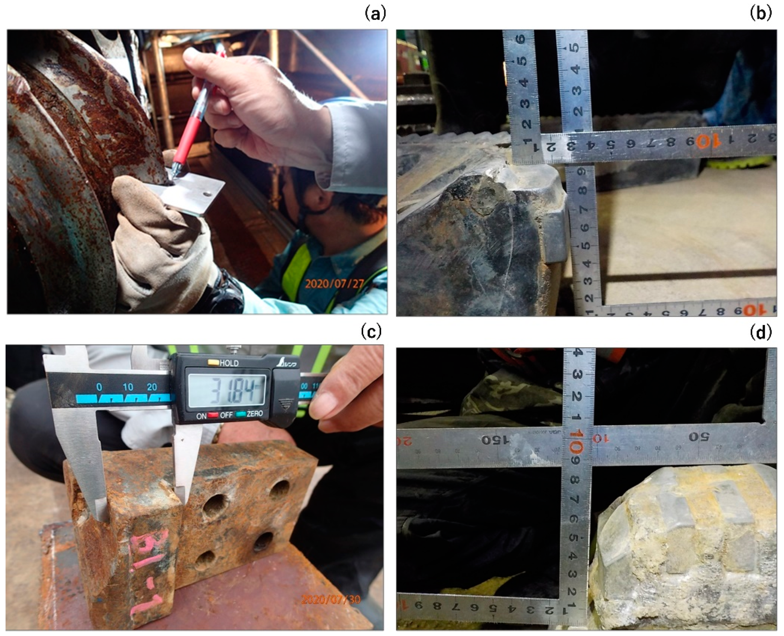
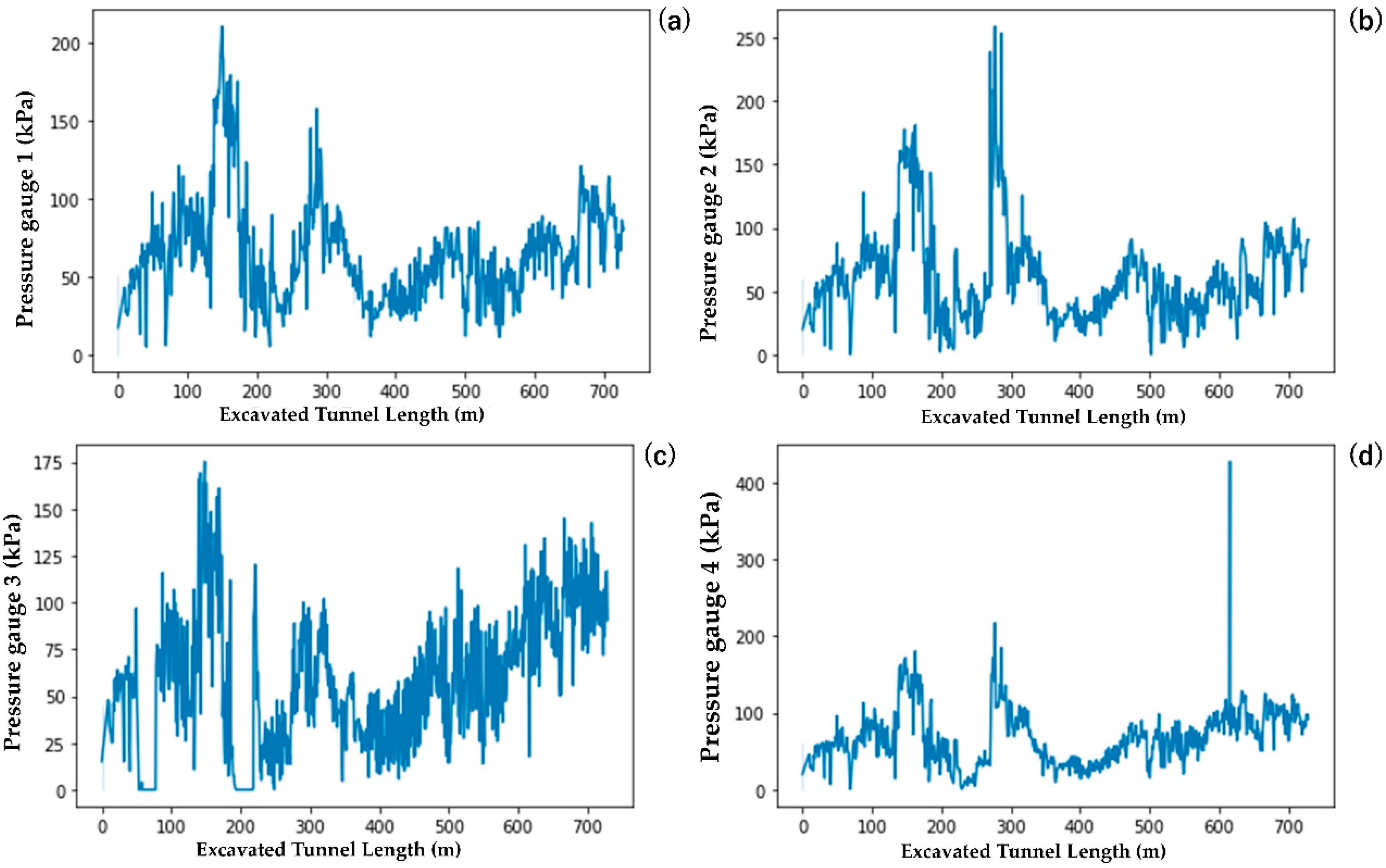
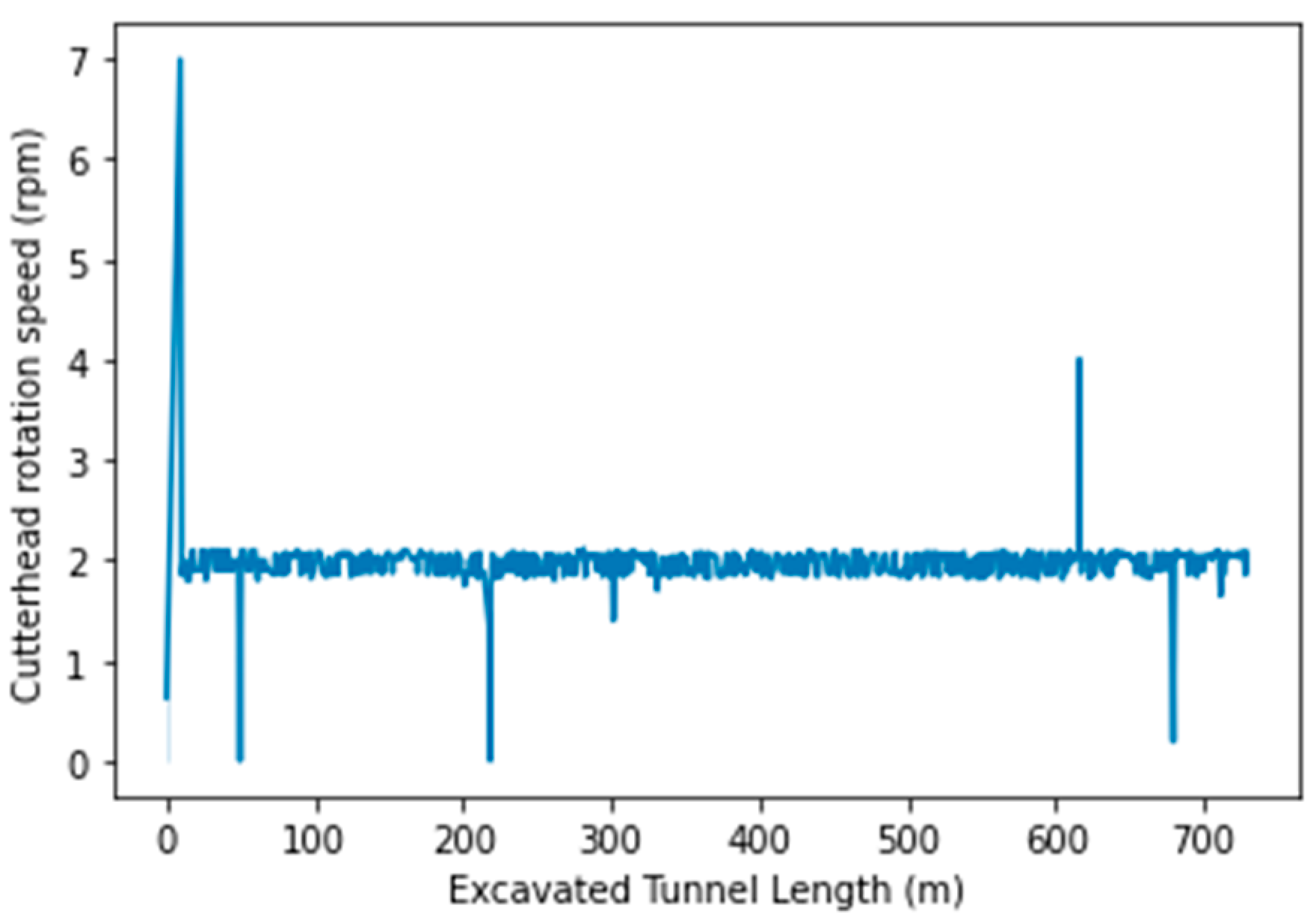
5. EPB Cutting Tool Wear and Machine Parameters

The EPB TBM (Figure 2) was dressed in different cutter tools, namely, a block bit, reamer bits, and disc cutters. Block bit tools are used to excavate nonabrasive soft-to-medium strength geological formations. Disc cutters are preferred for very dense, well-cemented soil and gravel boulders. Generally, disc cutters perform well in rock, but when a TBM excavates soft ground, disc cutters are exposed to frequent blockage and stop rotating. Therefore, disc cutters are faced with wear due to geological formation changes [41,42,43]. In this project, the total number of cutting tools changed to complete a full cutter head was 157: 52 disc cutters, 32 reamer bits, 68 block bits, and 5 leading bits. The cutter tools are shown in Figure 6, Figure 7, Figure 8 and Figure 9, respectively.

In previous studies [44,45], cutter life was defined as the amount of excavated material divided by the cutters consumed (${\mathrm{m}}^3/\mathrm{cutter})$, the hours of boring time divided by the cutters consumed ($\mathrm{hours}/\mathrm{cutter})$, and the excavated length by the total number of cutters ($\mathrm{m}/\mathrm{cutter})$. In this research, actual cutter life was obtained on the basis of excavated volume per disc cutter wear extent (${\mathrm{m}}^3/\mathrm{mm})$ due to the fine- or coarse-grained size of sandy gravel formation and normal or abnormal wear. Liu et al. [46] provided a prediction formula for the wear amount of disc cutter life to evaluate the normal and abnormal wear of disc cutters. The formula of the wear amount of the disc cutter is given in Equation (1).

$$E_f=\frac{\pi ·D^2·L}{4·M}$$

(1)

where D is the tunnel diameter, L is the excavated tunnel length, and M is the total amount of normal and abnormal disc cutter wear.

During the construction of the water tunnel project, all machine data were recorded in real time. While excavating the tunnel, 32 operational parameters were monitored and recorded. Among the 32 machine parameters, 18 machine parameters were selected for disc cutter wear as the input parameter of the 1D CNN regression model. A descriptive analysis of the machine parameters is shown in

Table 3. Descriptive machine parameters and output E_f (m³/mm).

Descriptive	Pressure Gauge (kPa)				Digging Velocity (mm/min)		Shield Jack Stroke (mm)		Propulsion Pressure (MPa)	Total Thrust (kN)	Cutter Torque (kN.m)	Cutter Rolling Velocity (rpm)	Screw Pressure (MPa)	Screw Rotation Speed (rpm)	Gate Opening (%)	Mud Injection Pressure (MPa)	Add MudFlow (L/min)	Back in injection rate (%)	Ef (m3/mm)
	1	2	3	4	Left	Right	Left	Right
Count	726	726	726	726	726	726	726	726	726	726	726	726	726	726	726	726	726	726	726
Mean	64.95	60.85	58.51	67.22	13.74	13.27	694.17	696.96	15.75	3459	482	1.96	2.85	0.90	29.40	0.18	16.33	96.9	39.79
Std	32.64	36.99	36.26	36.88	14.14	10.71	137.75	213.39	5.82	1268	69	0.27	5.42	2.96	12.16	0.08	8.24	37.71	22.6
Min	0	0	0	0	0	0	0	0	0	0	0	0	−114	−1.21	0	0	0	0	0
25%	42.43	35.90	31.63	39.75	8.18	8	692.27	689.31	11.36	2517	449	1.87	2.66	0.30	22.72	0.14	10.2	79.54	30.15
50%	60.45	53.90	56.13	64.19	12	12	700.5	699	14.90	3290	478	2	2.93	0.55	27.09	0.17	15.56	91.36	39.81
75%	80.79	76.81	84.38	88.43	17.34	16.90	706.63	707.15	19.97	4335	515	2.06	3.35	1.1	35.63	0.22	21.48	110.2	59.39
Max	210.27	259	175.36	426.93	336	239	3504.2	5946	31.54	7160	694	7	7.69	78.25	67.27	1.6	58.31	560	78.7

. The selected machine parameters are related to EPB TBM wear issues. Therefore, the thrust force, torque, cutter rolling speed, screw pressure, propulsion speed, screw rotation speed, four sides of earth pressure in the cutter chamber, two different shield jack strokes, gate opening, mud injection pressure, add mudflow, back in injection rate, digging velocity (left), and digging velocity (right) were determined to anticipate the disc cutter life. According to Sadegh et al. [41], thrust and torque are critical parameters for cutter life because, if the thrust and torque are higher than the requirement, cutter tools are exposed to brittle failure. Furthermore, based on the work of O’Carroll [42], if an EPB TBM is employed at a higher earth pressure than that required, the torque and excessive wear on the cutter head and cutting tools will increase. Moreover, Jakobsen and Lohne [47] proved that increasing cutter rolling speed impacts cutter wear. In addition to the thrust, torque, earth pressure in the cutter chamber, and cutter head rotation speed, the rest of the machine parameters have not been evaluated for cutter life prediction to date. Compared to the limited number of rock and soil parameters, machine parameters are high-dimensional and real-time data. According to Sadegh et al. and O’Carroll [41,42], there are only a few studies related to machine-parameter-based tool life prediction. Although empirical, probabilistic, and a few artificial intelligence models exist, there is no universal formula or research in this field.

Machine Parameters and Tool Wear Evaluation

Disc cutter life was predicted using each operational parameter obtained from each ring of the shield tunnelling. According to Hassanpour and Köppl et al. [5,48], the number of cutter changes was mostly applied in previous studies, whereas excavated volume per disc cutter wear extent (${\mathrm{m}}^3/\mathrm{mm})$ was only used in [46].

In this research, disc cutter wear was recorded at the end of four excavation lengths, namely, 205 m, 344 m, 493 m, and 623 m. The cutter tools’ wear amount was measured by a disc-measuring ruler and caliper on the tunnel site. The wear measurements of the disc cutters, reamer bits, block bits, and leading bits are shown in Figure 10a–d, respectively. However, in this study, only the disc cutters mounted on the EPB TBM cutter head were considered.

The total wear amount of the disc cutter tools is shown in

Table 4. Ring number and total wear amount of disc cutters.

Inspection Points	Total Wear (mm)
205	76
344	33
493	41
623	103
Total	253
M (arithmetic average)	63.3

. According to Equation (1), the total amount of the wear value (M) was obtained as an arithmetic average of the total amount of wear at inspection points 205, 344, 493, and 623. The (M) value was calculated using Equation (2).

$$M=\frac{1}{n}{{\displaystyle \sum }}_{i=1}^n{a}_i$$

(2)

where M is the arithmetic average of the total amount of cutter wear, n is the number of values, and $a_i$ is the total wear per ring number.

Furthermore, the EPB TBM thrust force and torque fluctuation in the excavated tunnel length are shown in Figure 11a,b, respectively. Due to the fluctuation of advancement forces, cutter tools are exposed to unplanned wear. Moreover, an EPB TBM works in a hyperbaric pressure environment, so proper stability pressure in the cutter chamber is another critical parameter for tool life. Figure 12a–d show pressure measurement in pressure gauges 1–4, respectively. The rpm of the cutter head is important for the penetration rate, and the EPB TBM rpm change is presented in Figure 13. The machine parameters were exposed to fluctuation due to the engineering geology discussed in Section 4.

6. Explanation of CNN

Aloysius and Geetha, and Albawi [49,50] explained that the convolutional neural network (CNN) was inspired by the visual cortex of animals. The CNN was initially utilized for object detection. Then, it was widely used in the deep neural network field for different applications, such as text detection, action recognition, classification, and regression analysis. Dhillon [51] stated that the CNN is composed of neurons, with each neuron having a learnable weight and bias. The CNN includes input layers, output layers, and multiple hidden layers. Hidden layers are formed by convolutional, pooling, fully connected, and normalization layers. The working principle of the convolutional layers is to merge two sets of information and then simulate the feedback of individual neurons to present visual stimuli. Another property of the CNN is pooling, which is implemented to decrease dimensionality. Furthermore, the fully connected layer works to connect one layer to every neuron in another layer. The initial purpose of the fully connected layer is to classify the input parameters into several classes on the basis of training data. A convolutional neural system indicates that the system uses a mathematical linear calculation called convolution instead of regular matrix multiplication in one or more layers.

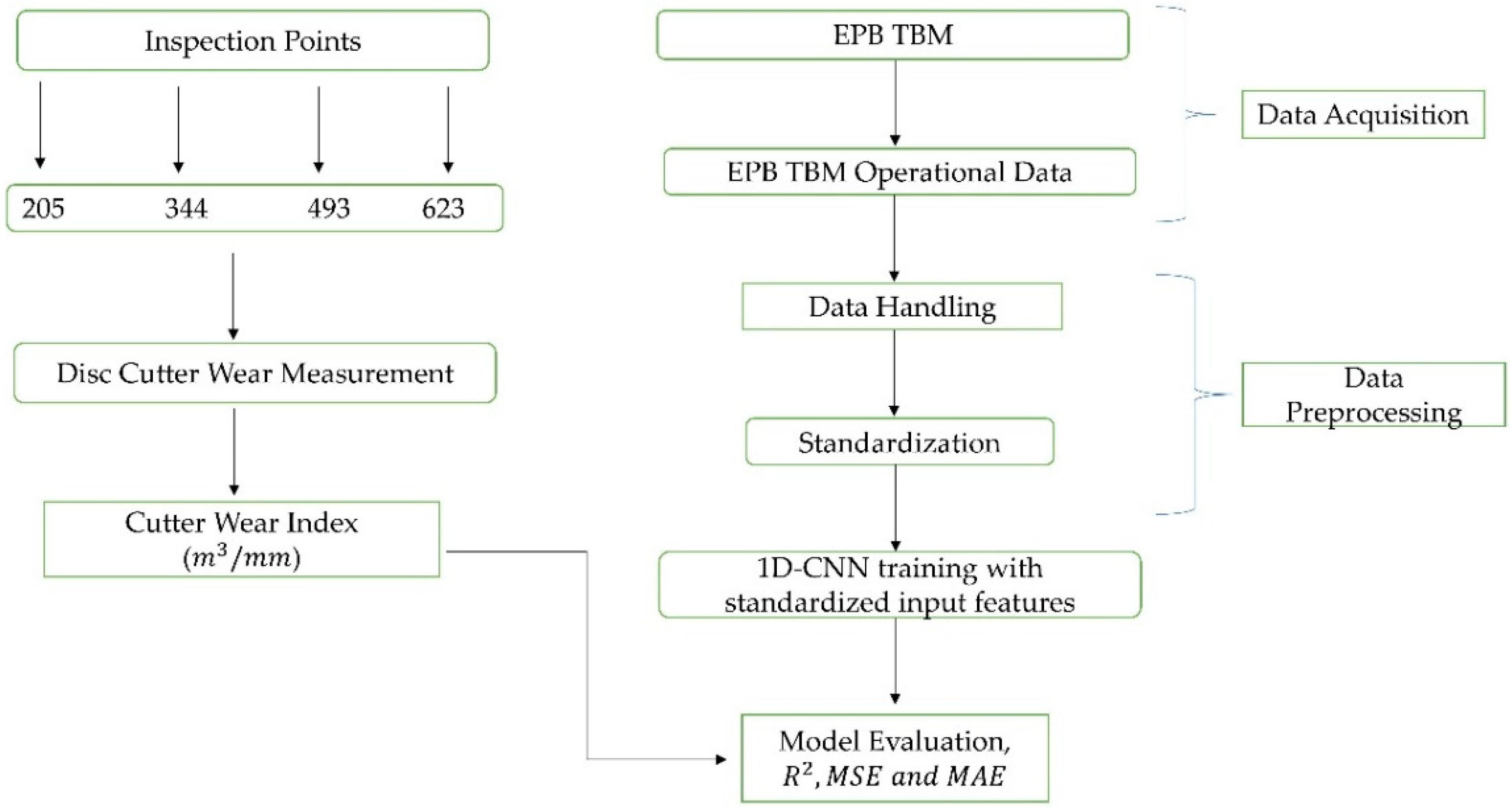
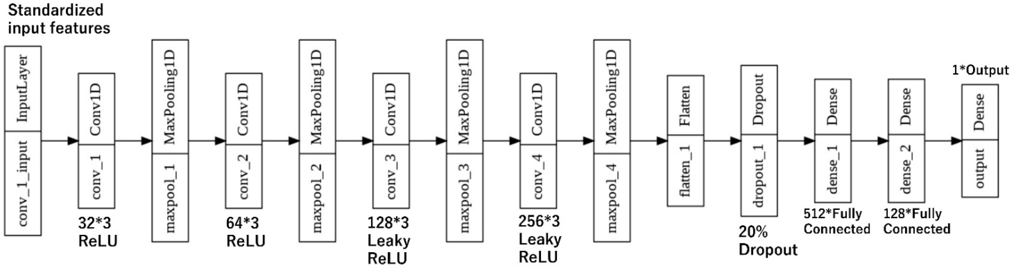
7. Proposed 1D CNN Regression for Cutter Wear Prediction

The CNN model is commonly used for classification tasks with category-based datasets. However, CNNs are rarely applied to numerical values and regression analysis. Therefore, the traditional CNN model was merged with the regression problem due to the numerical input and output data. The proposed 1D CNN regression architecture was used for high-dimensional regression analysis, and the 1D CNN model was inspired by [36,52]. Moreover, to reduce training time and to obtain a shorter computational time for fully connected layers, the kernel size was set to 3 [53]. Furthermore, the filter size (count) is the power of two between 32 and 1024. Even though a high filter size can create a powerful model, it can lead to overfitting. For this reason, 32, 64, 128, and 256 filter sizes were chosen for our model. However, the proposed 1D CNN model architecture and hyperparameters were constructed to suit the EPB TBM numerical dataset using Python Keras-Tensorflow. The proposed 1D CNN model architecture is shown in Figure 14. Before model training, the data were split; 80% of the data were used for training, and 20% of the data were tested. The CNN model was created using four convolutional layers within four max-pooling layers. The 1D CNN architecture was obtained by trial and error on the basis of correlation coefficient and loss function mean square error. The first convolutional layer consisted of 32 filter sizes, 3 kernel sizes, and the ReLU activation function. The second convolutional layer included 64 filter sizes, 3 kernel sizes, and the ReLU activation function. The third and the fourth convolutional layers comprised 128 filter sizes, 3 kernel sizes, and the Leaky ReLU activation function, and 256 filter sizes and 3 kernel sizes within the Leaky ReLU activation function, respectively. After convolutional and max-pooling layers, the flatten layer was implemented to transform the data into a single vector. To avoid overfitting, the dropout function was utilized with 20%. After dropout, there were two fully connected layers with 512 and 128 filter sizes and the Leaky ReLU activation function before the output layer. The output layer was one filter size with the linear activation function due to the one output. For the model compilation, the loss function was determined as the mean square error, and the model metric was selected as the mean absolute error. The Keras’ Adam function was performed as a model optimizer. Moreover, the Adam function is a stochastic gradient-descent-based optimizer, and it provides avoidance of the local minimum trap. A summary of the proposed CNN model is shown in

Table 5. Proposed 1D CNN model summary.

Layer	Output Shape	Parameters
Conv_1 (1D)	(None, 1532)	128
MaxPooling1D	(None, 1532)	0
Conv_2 (1D)	(None, 1364)	6208
MaxPooling1D	(None, 1364)	0
Conv_3 (1D)	(None, 11,128)	24,704
MaxPooling1D	(None, 11,128)	0
Conv_4 (1D)	(None, 9256)	98,560
MaxPooling1D	(None, 9256)	0
Flatten	(None, 2304)	0
Dense_1	(None, 512)	1,180,160
Dense_2	(None, 128)	65,664
Output (Dense)	(None, 1)	129
Trainable Params	1,375,553

“None” refers to the batch size of the model.

. The 1D CNN model has a total of 1,375,553 trainable parameters with 5 batch sizes and 100 epoch sizes. The proposed 1D CNN model computational time (wall time) is 3 min 22 s, so the deep learning model provides a fast calculation for a large dataset. The important CNN activation and loss functions are described in Section 7.1, Section 7.2, Section 7.3, Section 7.4, Section 7.5 and Section 7.6.

7.1. Data Preprocessing

Before model training and data splitting, the EPB TBM machine parameters were standardized using Equation (3).

$$z=\frac{x-\mu }{\sigma }$$

(3)

where $\mu$ is the mean, $\sigma$ is the standard deviation of the input parameters, and z is an element of the normalized training data.

7.2. ReLU Function

The rectified linear unit (ReLU) is a linear activation function with zero thresholds as in Equation (4). The convergence of the gradient descent can be accelerated by applying ReLU [49,50]. The ReLU function is used for negative values in the dataset to return 0. Furthermore, the ReLU function was utilized to obtain easier training and high model performance.

$$\begin{gathered} ReLU\left(x\right)=\max \left(0,x\right) \\ \frac{d}{dx}\left(x\right)=\{1ifx>0;0otherwise\} \end{gathered}$$

(4)

7.3. Leaky ReLU

The leaky ReLU is a slightly adjusted version of the ReLU function and is shown in Equation (5) [49].

$$f\left(x\right)=\{\begin{array}{c}x, x\le 0\\ 0.01x, otherwise\end{array}$$

(5)

7.4. Mean Squared Error (MSE)

The mean squared error (MSE) function was used as a loss layer in the convolutional neural network to compute the loss or error between the actual and predicted output. The MSE was proposed for the regression task. Equation (6) presents the MSE loss function [54].

$$MSE=\frac{1}{n}{\displaystyle \sum }_{i=1}^n\left(y_i-{\widehat{y}}_i\right)$$

(6)

where n refers to the size of the test dataset, $y_i$ is the actual output, and ${\widehat{y}}_i$ is the predicted output.

7.5. Mean Absolute Error (MAE)

The mean absolute error (MAE) function was used as a metric of the output layer in the proposed convolutional neural network. The MAE shows the percentage of the estimated variables. Equation (7) expresses the MAE formula [55].

$$MAE=\frac{1}{n}{\displaystyle \sum }_{i=1}^n\left(y_i-{\widehat{y}}_i\right)$$

(7)

7.6. Regularization

The regularization layer was implemented in the convolutional neural network model to avoid overfitting while model training. The name of the application was Dropout, and the Dropout value was set to 20% for the proposed 1D CNN model. Each hidden unit was arbitrarily omitted from the network with a likelihood of 0.2; thus, a hidden layer unit could not rely on other hidden layers being represented [52,55].

8. Model Comparison

The 1D CNN regression model performance was considered using the mean squared error (MSE), mean absolute error (MAE), and correlation coefficient ($R^2$) evaluation metrics. The MSE and MAE metrics are described in Equations (6) and (7), respectively. The model prediction and corresponding actual distribution with the fit line are shown in Figure 15a. Figure 15b illustrates the error between the predicted and actual cutter wear with a histogram. Figure 15c presents the 1D CNN learning curve with 100 epochs. The reliable performance of the 1D CNN model was proved through a comparison of the six machine learning models (extratree regression, light gradient boosting, gradient boosting, random forest, AdaBoost, and k-NN regression) and two deep neural network models (MLP and LSTM).

Table 6. Model comparison.

Model	${\mathit{R}}^2$	MSE	MAE	Time
Proposed 1D CNN	89.6	57.5	1.6	3 min 22 s
MLPRegressor	77.8	107	5.93	3 min 26 s
LSTMRegressor	39	326.3	11.12	12 min 38 s
Extratree regression	77.90	111.16	7.31	0.497 s
Light gradient boosting machine	73.98	130.19	8.04	0.101 s
Gradient boosting machine	71.81	141.01	8.71	0.182 s
Random forest regression	70.72	147.54	8.35	0.671 s
AdaBoost regressor	59.12	202.48	11.84	0.127 s
k-NN regression	19.04	452.03	15.47	0.062 s

presents a comparison of the proposed 1D CNN (deep learning), long short-term memory (LSTM), multilayer perceptron (MLP) neural network, and the six traditional machine learning models.

The results illustrate that in terms of the correlation coefficient, mean squared error (MSE), and mean absolute error (MAE), the proposed model performed better than the six traditional machine learning models and the two deep neural networks models. The proposed 1D CNN model had a correlation coefficient of 89.6%, a mean squared error of 57.5, and a mean absolute error of 1.6. The k-NN regression had the lowest correlation coefficient of 19.04%. In terms of the neural network comparison, the LSTMRegressor had the lowest correlation coefficient of 39% and the highest prediction error value of 326.3 MSE. Based on computational time, k-NN regression had the best performance, by taking the shortest time of 0.062 s. Moreover, the proposed 1D CNN model had the fastest computational time of 3 min 22 s compared to the MLPRegressor (3 min 26 s) and the LSTMRegressor (12 min 38 s). The proposed 1D CNN model outperforms the traditional machine learning models and the two different neural network models in terms of the correlation coefficient, MSE, MAE, and computational efficiency, which makes it superior in estimating soft ground cutter wear with operational data in EPB TBM tunnelling.

9. Discussion

The soil parameters in Table 2 indicate a transition in the soil from a cohesive soil to a coarser soil. Due to soft ground feature transition, the EPB TBM machine parameters are exposed to fluctuation, and they are shown in Figure 11, Figure 12 and Figure 13. Utilizing these operational parameters with the EPB TBM operator allows for an increase in machine advancement parameters, such as thrust and torque. Therefore, the EPB TBM cutter tools experience damage and wear. Figure 12a–d show the pressure in the cutter chamber along with the tunnel. Moreover, Figure 5 indicates the difference in grain size characteristics. Due to the grain size characteristics, the pressures in the cutter chamber demonstrate a sharp fluctuation during excavation. To control the pressure in the cutter chamber, the TBM operator tends to increase the thrust, RPM, and torque. It is obvious that the operational parameters influence cutter wear during tunnel excavation. Furthermore, by using the proposed 1D CNN model on the operational data collected from the pipe jacking water transport tunnel project, an attempt was made to provide a fast and practical estimation for the cutter wear of the EPB TBM by employing high-dimensional machine parameters. The proposed 1D CNN indicated a strong correlation between the machine parameters and cutter wear index (${\mathrm{m}}^3$/mm). The 1D CNN model can be implemented in soft ground mechanized tunnelling projects to predict cutter wear and excavation efficiency. However, it should be noted that current studies are far from providing a universal model for cutter wear in soft ground TBMs.

10. Conclusions

This research employed the operational parameters of an EPB TBM and a 1D CNN to build a reliable normal and abnormal cutter wear prediction model. The EPB TBM advancement parameters and the pressure in the cutter chamber were considered, as we aimed to build a cost-effective, highly reliable model with fast computation. The 1D CNN model was used due to its abilities to optimize the parameters in the case of global and local minima and automatic feature extraction for the output. A four convolutional CNN model with 256 filters, 3 kernel sizes, 20% dropout, 2 fully connected layers, and the Adam optimizer was utilized to estimate cutter wear using machine parameters. The model had an overall correlation coefficient of 89.6%, a mean squared error (MSE) of 57.5, and a mean absolute error of 1.6. The model was able to successfully predict the cutter tool’s life with a fast computational time, which was 3 min 22 s. We demonstrated that the proposed model could achieve a better prediction and processing time than that of traditional machine learning models and two deep neural network models. In application, the cutter wear prediction model could be used at the inspection points of the tunnel by the TBM operator to gain an understanding of the machine parameters and wearing relationship. Moreover, this study is the first to apply deep learning to cutter wear prediction in soft ground tunnelling. In this study, 18 different machine parameters were considered; in the future, more operational parameters can be used to develop deep learning models; hard rock and soft ground machine parameters can be used with pre-trained models to validate model computational ability.

References

1. Feng, S.; Chen, Z.; Luo, H.; Wang, S.; Zhao, Y.; Liu, L.; Ling, D.; Jing, L. Tunnel Boring Machines (TBM) Performance Prediction: A Case Study Using Big Data and Deep Learning. Tunn. Undergr. Space Technol. 2021, 110, 103636. [Google Scholar] [CrossRef]
2. Hartlieb, P.; Grafe, B.; Shepel, T.; Malovyk, A.; Akbari, B. Experimental Study on Artificially Induced Crack Patterns and Their Consequences on Mechanical Excavation Processes. Int. J. Rock Mech. Min. Sci. 2017, 100, 160–169. [Google Scholar] [CrossRef]
3. Zhang, X.; Xia, Y.; Zhang, Y.; Tan, Q.; Zhu, Z.; Lin, L. Experimental Study on Wear Behaviors of TBM Disc Cutter Ring under Drying, Water and Seawater Conditions. Wear 2017, 392–393, 109–117. [Google Scholar] [CrossRef]
4. Ren, D.-J.; Shen, S.-L.; Arulrajah, A.; Cheng, W.-C. Prediction Model of TBM Disc Cutter Wear during Tunnelling in Heterogeneous Ground. Rock Mech. Rock Eng. 2018, 51, 3599–3611. [Google Scholar] [CrossRef]
5. Hassanpour, J.; Rostami, J.; Tarigh Azali, S.; Zhao, J. Introduction of an Empirical TBM Cutter Wear Prediction Model for Pyroclastic and Mafic Igneous Rocks; a Case History of Karaj Water Conveyance Tunnel, Iran. Tunn. Undergr. Space Technol. 2014, 43, 222–231. [Google Scholar] [CrossRef]
6. Barzegari, G.; Khodayari, J.; Rostami, J. Evaluation of TBM Cutter Wear in Naghadeh Water Conveyance Tunnel and Developing a New Prediction Model. Rock Mech. Rock Eng. 2021, 54, 6281–6297. [Google Scholar] [CrossRef]
7. Wang, R.; Wang, Y.; Li, J.; Jing, L.; Zhao, G.; Nie, L. A TBM Cutter Life Prediction Method Based on Rock Mass Classification. KSCE J. Civ. Eng. 2020, 24, 2794–2807. [Google Scholar] [CrossRef]
8. Rong, X.; Lu, H.; Wang, M.; Wen, Z.; Rong, X. Cutter Wear Evaluation from Operational Parameters in EPB Tunneling of Chengdu Metro. Tunn. Undergr. Space Technol. 2019, 93, 103043. [Google Scholar] [CrossRef]
9. Su, W.; Li, X.; Jin, D.; Yang, Y.; Qin, R.; Wang, X. Analysis and Prediction of TBM Disc Cutter Wear When Tunneling in Hard Rock Strata: A Case Study of a Metro Tunnel Excavation in Shenzhen, China. Wear 2020, 446–447, 203190. [Google Scholar] [CrossRef]
10. Jamal, R.; Ozdemir, L. New model for performance production of hard rock TBMs. In Proceedings of the Rapid Excavation and Tunneling Conference, Boston, MA, USA, 1 January 1993; pp. 793–809. [Google Scholar]
11. Bruland, A. Hard Rock Tunnel Boring; Norwegian University of Science and Technology: Trondheim, Norway, 2000. [Google Scholar]
12. Roxborough, F.F.; Phillips, H.R. Rock Excavation by Disc Cutter. Int. J. Rock Mech. Min. Sci. Geomech. Abstr. 1975, 12, 361–366. [Google Scholar] [CrossRef]
13. Wijk, G. A Model of Tunnel Boring Machine Performance. Geotech. Geol. Eng. 1992, 10, 19–40. [Google Scholar] [CrossRef]
14. Barton, N.R. TBM Tunnelling in Jointed and Faulted Rock; CRC Press: Boca Raton, FL, USA, 2000; p. 184. [Google Scholar]
15. Cardu, M.; Iabichino, G.; Oreste, P.; Rispoli, A. Experimental and Analytical Studies of the Parameters Influencing the Action of TBM Disc Tools in Tunnelling. Acta Geotech. 2017, 12, 293–304. [Google Scholar] [CrossRef]
16. Zare, S.; Bruland, A. Applications of NTNU/SINTEF Drillability Indices in Hard Rock Tunneling. Rock Mech. Rock Eng. 2013, 46, 179–187. [Google Scholar] [CrossRef]
17. Macias, F.J.; Dahl, F.; Bruland, A. New Rock Abrasivity Test Method for Tool Life Assessments on Hard Rock Tunnel Boring: The Rolling Indentation Abrasion Test (RIAT). Rock Mech. Rock Eng. 2016, 49, 1679–1693. [Google Scholar] [CrossRef]
18. Ko, T.Y.; Lee, S.S. Effect of Rock Abrasiveness on Wear of Shield Tunnelling in Bukit Timah Granite. Appl. Sci. 2020, 10, 3231. [Google Scholar] [CrossRef]
19. Farrokh, E. Primary and Secondary Tools’ Life Evaluation for Soft Ground TBMs. Bull. Eng. Geol. Environ. 2021, 80, 4909–4927. [Google Scholar] [CrossRef]
20. Alvarez Grima, M.; Bruines, P.A.; Verhoef, P.N.W. Modeling Tunnel Boring Machine Performance by Neuro-Fuzzy Methods. Tunn. Undergr. Space Technol. 2000, 15, 259–269. [Google Scholar] [CrossRef]
21. Benardos, A.G.; Kaliampakos, D.C. Modelling TBM Performance with Artificial Neural Networks. Tunn. Undergr. Space Technol. 2004, 19, 597–605. [Google Scholar] [CrossRef]
22. Yagiz, S.; Gokceoglu, C.; Sezer, E.; Iplikci, S. Application of Two Non-Linear Prediction Tools to the Estimation of Tunnel Boring Machine Performance. Eng. Appl. Artif. Intell. 2009, 22, 808–814. [Google Scholar] [CrossRef]
23. Ghasemi, E.; Yagiz, S.; Ataei, M. Predicting Penetration Rate of Hard Rock Tunnel Boring Machine Using Fuzzy Logic. Bull. Eng. Geol. Environ. 2014, 73, 23–35. [Google Scholar] [CrossRef]
24. Mahdevari, S.; Shahriar, K.; Yagiz, S.; Akbarpour Shirazi, M. A Support Vector Regression Model for Predicting Tunnel Boring Machine Penetration Rates. Int. J. Rock Mech. Min. Sci. 2014, 72, 214–229. [Google Scholar] [CrossRef]
25. Mahdevari, S.; Torabi, S.R.; Monjezi, M. Application of Artificial Intelligence Algorithms in Predicting Tunnel Convergence to Avoid TBM Jamming Phenomenon. Int. J. Rock Mech. Min. Sci. 2012, 55, 33–44. [Google Scholar] [CrossRef]
26. Shao, C.; Li, X.; Su, H. Performance Prediction of Hard Rock TBM Based on Extreme Learning Machine. In Proceedings of the International Conference on Intelligent Robotics and Applications, Busan, Korea, 25–28 September 2013; Lee, J., Lee, M.C., Liu, H., Ryu, J.-H., Eds.; Lecture Notes in Computer Science. Springer: Berlin/Heidelberg, Germany, 2013; pp. 409–416. [Google Scholar] [CrossRef]
27. Salimi, A.; Faradonbeh, R.S.; Monjezi, M.; Moormann, C. TBM Performance Estimation Using a Classification and Regression Tree (CART) Technique. Bull. Eng. Geol. Environ. 2018, 77, 429–440. [Google Scholar] [CrossRef]
28. Koopialipoor, M.; Nikouei, S.S.; Marto, A.; Fahimifar, A.; Jahed Armaghani, D.; Mohamad, E.T. Predicting Tunnel Boring Machine Performance through a New Model Based on the Group Method of Data Handling. Bull. Eng. Geol. Environ. 2019, 78, 3799–3813. [Google Scholar] [CrossRef]
29. Koopialipoor, M.; Tootoonchi, H.; Jahed Armaghani, D.; Tonnizam Mohamad, E.; Hedayat, A. Application of Deep Neural Networks in Predicting the Penetration Rate of Tunnel Boring Machines. Bull. Eng. Geol. Environ. 2019, 78, 6347–6360. [Google Scholar] [CrossRef]
30. Jahed Armaghani, D.; Faradonbeh, R.S.; Momeni, E.; Fahimifar, A.; Tahir, M.M. Performance Prediction of Tunnel Boring Machine through Developing a Gene Expression Programming Equation. Eng. Comput. 2018, 34, 129–141. [Google Scholar] [CrossRef]
31. Yang, H.; Wang, Z.; Song, K. A New Hybrid Grey Wolf Optimizer-Feature Weighted-Multiple Kernel-Support Vector Regression Technique to Predict TBM Performance. Eng. Comput. 2020, 1–17. [Google Scholar] [CrossRef]
32. Li, J.; Li, P.; Guo, D.; Li, X.; Chen, Z. Advanced Prediction of Tunnel Boring Machine Performance Based on Big Data. Geosci. Front. 2021, 12, 331–338. [Google Scholar] [CrossRef]
33. Elbaz, K.; Shen, S.-L.; Zhou, A.; Yuan, D.-J.; Xu, Y.-S. Optimization of EPB Shield Performance with Adaptive Neuro-Fuzzy Inference System and Genetic Algorithm. Appl. Sci. 2019, 9, 780. [Google Scholar] [CrossRef] [Green Version]
34. Mahmoodzadeh, A.; Mohammadi, M.; Hashim Ibrahim, H.; Nariman Abdulhamid, S.; Farid Hama Ali, H.; Mohammed Hasan, A.; Khishe, M.; Mahmud, H. Machine Learning Forecasting Models of Disc Cutters Life of Tunnel Boring Machine. Autom. Constr. 2021, 128, 103779. [Google Scholar] [CrossRef]
35. Massalov, T.; Yagiz, S.; Adoko, A.C. Application of Soft Computing Techniques to Estimate Cutter Life Index Using Mechanical Properties of Rocks. Appl. Sci. 2022, 12, 1446. [Google Scholar] [CrossRef]
36. Yu, H.; Tao, J.; Huang, S.; Qin, C.; Xiao, D.; Liu, C. A Field Parameters-Based Method for Real-Time Wear Estimation of Disc Cutter on TBM Cutterhead. Autom. Constr. 2021, 124, 103603. [Google Scholar] [CrossRef]
37. Elbaz, K.; Shen, S.-L.; Zhou, A.; Yin, Z.-Y.; Lyu, H.-M. Prediction of Disc Cutter Life during Shield Tunneling with AI via the Incorporation of a Genetic Algorithm into a GMDH-Type Neural Network. Engineering 2021, 7, 238–251. [Google Scholar] [CrossRef]
38. Obara, H.; Maejima, Y.; Kohyama, K.; Ohkura, T.; Takata, Y. Outline of the Comprehensive Soil Classification System of Japan–First Approximation. Jpn. Agric. Res. Q. 2015, 49, 217–226. [Google Scholar] [CrossRef] [Green Version]
39. Hirai, H.; Hamazaki, T. Historical Aspects of Soil Classification in Japan. Soil Sci. Plant 2004, 50, 611–622. [Google Scholar] [CrossRef]
40. Park, J.; Santamarina, J.C. Revised Soil Classification System for Coarse-Fine Mixtures. J. Geotech. Geoenviron. 2017, 143, 04017039. [Google Scholar] [CrossRef] [Green Version]
41. Amoun, S.; Sharifzadeh, M.; Shahriar, K.; Rostami, J.; Tarigh Azali, S. Evaluation of Tool Wear in EPB Tunneling of Tehran Metro, Line 7 Expansion. Tunn. Undergr. Space Technol. 2017, 61, 233–246. [Google Scholar] [CrossRef]
42. O’Carroll, J.B. A Guide to Planning, Constructing, and Supervising Earth Pressure Balance TBM Tunneling; Parsons Brinckerhoff: New York, NY, USA, 2005. [Google Scholar]
43. Bilgin, N.; Copur, H.; Balci, C. Mechanical Excavation in Mining and Civil Industries; CRC Press: Boca Raton, FL, USA, 2013; pp. 49–120. [Google Scholar]
44. Hassanpour, J.; Rostami, J.; Zhao, J.; Azali, S.T. TBM Performance and Disc Cutter Wear Prediction Based on Ten Years Experience of TBM Tunnelling in Iran. Geomech. Tunn. 2015, 8, 239–247. [Google Scholar] [CrossRef]
45. Bruland, A. Hard rock tunnel boring: Drillability test methods. In Project Report 13A-98, NTNU Trondheim 21; Academia: San Francisco, CA, USA, 1998. [Google Scholar]
46. Liu, Q.; Liu, J.; Pan, Y.; Zhang, X.; Peng, X.; Gong, Q.; Du, L. A Wear Rule and Cutter Life Prediction Model of a 20-in. TBM Cutter for Granite: A Case Study of a Water Conveyance Tunnel in China. Rock Mech. Rock Eng. 2017, 50, 1303–1320. [Google Scholar] [CrossRef]
47. Jakobsen, P.D.; Lohne, J. Challenges of Methods and Approaches for Estimating Soil Abrasivity in Soft Ground TBM Tunnelling. Wear 2013, 308, 166–173. [Google Scholar] [CrossRef]
48. Köppl, F.; Thuro, K.; Thewes, M. Suggestion of an Empirical Prognosis Model for Cutting Tool Wear of Hydroshield TBM. Tunn. Undergr. Space Technol. 2015, 49, 287–294. [Google Scholar] [CrossRef]
49. Albawi, S.; Mohammed, T.A.; Al-Zawi, S. Understanding of a Convolutional Neural Network. In Proceedings of the 2017 International Conference on Engineering and Technology (ICET), Antalya, Turkey, 21–23 August 2017; pp. 1–6. [Google Scholar] [CrossRef]
50. Aloysius, N.; Geetha, M. A Review on Deep Convolutional Neural Networks. In Proceedings of the 2017 International Conference on Communication and Signal Processing (ICCSP), Tamilnadu, India, 6–8 April 2017; pp. 0588–0592. [Google Scholar] [CrossRef]
51. Dhillon, A.; Verma, G.K. Convolutional Neural Network: A Review of Models, Methodologies and Applications to Object Detection. Prog. Artif. Intell. 2020, 9, 85–112. [Google Scholar] [CrossRef]
52. Fu, X.; Zhang, C.; Peng, X.; Jian, L.; Liu, Z. Towards End-to-End Pulsed Eddy Current Classification and Regression with CNN. In Proceedings of the 2019 IEEE International Instrumentation and Measurement Technology Conference (I2MTC), Auckland, New Zealand, 20–23 May 2019; pp. 1–5. [Google Scholar] [CrossRef] [Green Version]
53. Simonyan, K.; Zisserman, A. Very Deep Convolutional Networks for Large-Scale Image Recognition. arXiv 2015, arXiv:1409.1556. [Google Scholar]
54. Khan, Z.A.; Hussain, T.; Ullah, A.; Rho, S.; Lee, M.; Baik, S.W. Towards Efficient Electricity Forecasting in Residential and Commercial Buildings: A Novel Hybrid CNN with a LSTM-AE Based Framework. Sensors 2020, 20, 1399. [Google Scholar] [CrossRef] [Green Version]
55. Hinton, G.E.; Srivastava, N.; Krizhevsky, A.; Sutskever, I.; Salakhutdinov, R.R. Improving Neural Networks by Preventing Co-Adaptation of Feature Detectors. arXiv 2012, arXiv:1207.0580. [Google Scholar]
Figure 1. Overview of the proposed disc cutter wear prediction model. The proposed 1D CNN model was trained and evaluated to obtain the best model for disc cutter wear prediction.
Applsci 12 02410 g001
Figure 2. Cutter arrangement of EPB TBM.
Applsci 12 02410 g002
Figure 3. Tunnel geology: (a) entrance shaft, (b) middle shaft, (c) reaching shaft.
Applsci 12 02410 g003
Figure 4. Engineering geology tunnel profile.
Applsci 12 02410 g004
Figure 5. Triangular grain size distribution and characteristics: (a) Triangular system, (b) triangular coordinates for medium classification, (c) subclassification of coarse soil and fine-grained soil.
Applsci 12 02410 g005
Figure 6. Disc cutter tools.
Applsci 12 02410 g006
Figure 7. Reamer bits.
Applsci 12 02410 g007
Figure 8. Block bits.
Applsci 12 02410 g008
Figure 9. Leading bits.
Applsci 12 02410 g009
Figure 10. (a) Disc cutter, (b) reamer bit, (c) block bit, and (d) leading bit wear measurement on site.
Applsci 12 02410 g010
Figure 11. (a) Total thrust (kN) and (b) cutter torque (kN.m).
Applsci 12 02410 g011
Figure 12. (a) Pressure 1, (b) Pressure 2, (c) Pressure 3, and (d) Pressure 4.
Applsci 12 02410 g012
Figure 13. Cutter head rotation speed (rpm).
Applsci 12 02410 g013
Figure 14. Proposed 1D CNN model architecture diagram.
Applsci 12 02410 g014
Figure 15. (a) Actual and predicted data distribution with fit line; (b) error distribution between actual and predicted data; (c) 1D CNN learning curve.
Applsci 12 02410 g015