Development of an On-Line Defect Detection System for EDM Process

Abstract

In the electrical discharge machining process, preliminary research has been able to effectively estimate machining accuracy in response to its long machining history and high discharge frequency characteristics. However, when processing abnormalities occur, it is difficult to identify them since the electrical discharge process contains multiple processing parameters, which increases the cost of repair or loss afterwards. Therefore, the question concerning how to monitor the abnormality of the discharge process in real time represents the main purpose of this research. This research develops an EDM process abnormal diagnosis system. First, the data are stored in a circular array to speed up the processing time, and the coefficient of variation feature is added, which has effectively extracted the abnormal characteristics. In terms of diagnostic methods, the composite voting model established by neural networks, random forests, and XGB-RF (extreme gradient boosting applying RF) can provide robust diagnostic results. Finally, through the Node-RED webpage and MQTT agreement, it can provide the ability to monitor machine abnormalities in real time. Through refinement and optimization of the previous research results, this study took the electrical discharge machining diamond grinding wheel as an example, and developed a warning that can be issued within 3 min when abnormalities (abnormal patterns such as polycrystalline diamond high protrusions) occur, with an accuracy of 93% and a false positive rate. The abnormal diagnosis ability is less than 0.2%. Therefore, the online abnormality monitoring system developed by this research institute will be able to provide online abnormality diagnosis for electrical discharge machining.

1. Introduction

The electrical discharge machining process applies pulse voltage to perform spark discharge, and uses the consumption that occurs at this time to process. The electrode and the workpiece are not in direct contact, and between the gap voltage is intervened by the electrical discharge fluid. So, the electrical discharge machining is applied for the material, which usually was difficult to machine by traditional cutting with higher hardness and precision. In terms of processing characteristics, Selvarajan et al. [1] pointed out three typical indicators of material removal rate, electrode consumption rate, and surface roughness. The three indicators were affected by peak current, peak voltage, discharge cycle time, polarity, discharge gap, etc. The workpiece in this study is a diamond grinding wheel, which has become a substitute for traditional cutting tools and is widely used in manufacturing, especially for processing alloys and glass. Based on its high hardness, good impact resistance, wear resistance, and excellent heat resistance and thermal conductivity [2], these characteristics mentioned above are suitable for electrical discharge machining. The surface material of the diamond grinding wheel is polycrystalline diamond (PCD). PCD is made of synthetic diamond and then sintered under high temperature and high pressure. Jia et al. [3] proposed that PCD crystals were arranged disorderly, isotropic, and without a cleavage plane. There are two main processing methods for refurbishing PCD. One is cutting and grinding, but it is difficult to achieve tapered edges and complex shapes, and this method has other problems such as the potential for serious wear. The other is EDM, which is simple to process conductive material parts and has low loss. EDM can be used effectively for the processing of complex shapes in PCD.

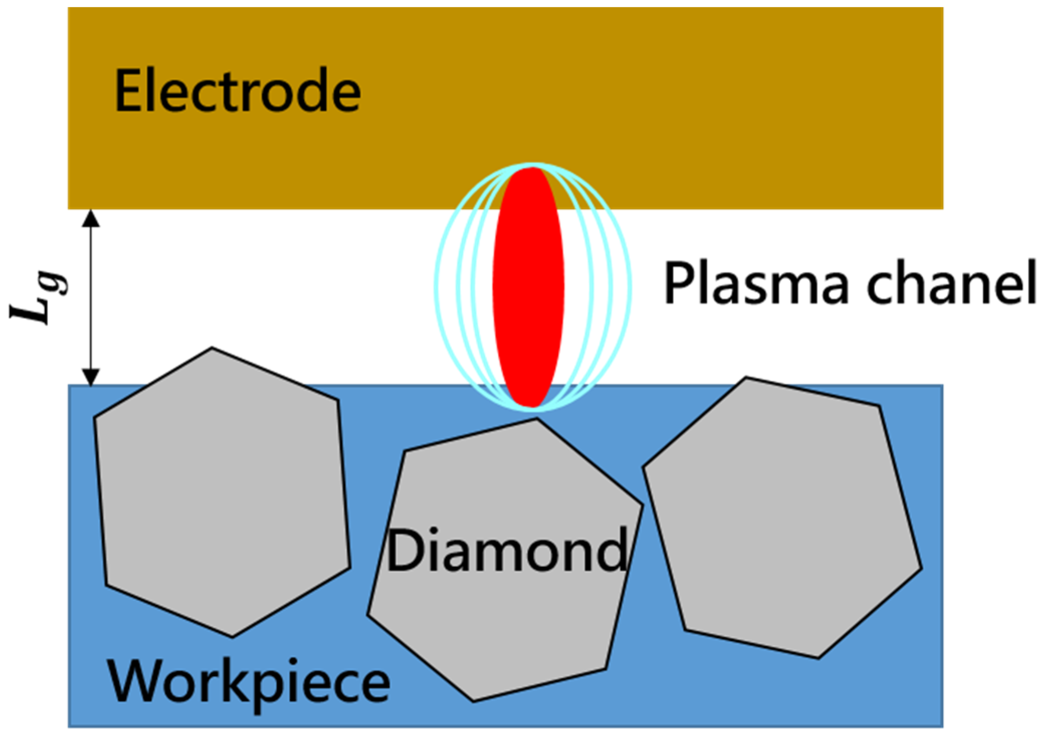
The principle of EDM processing PCD is shown in Figure 1. As the controller controls the feed rate, the gap (L_g) between the electrode and the workpiece changes accordingly. The electrode (positive electrode) and the surface of the workpiece (negative electrode) are rich in a large number of cations and anions, which are, respectively, affected by the electric field. As the intensity of the electric field increases, electrons are conducted to the surface of the workpiece to form a loop. Wang et al. [4] proposed that when EDM processed PCD, there was a graphene film on top of the PCD, and the discharge point was not restricted by the metal binder or limited to conductive materials (which was the case of conventional EDM). The discharge point could work on any surfaces of the piece theoretically. Therefore, this increased the occurrence of effective discharge pulses and contributes to an increase in material removal rate. According to Pei et al. [5], when a discharge spark occurred, the electric field strength between the electrodes reaches the strength of the dielectric breakdown. Avalanche ionization and collision dielectric would then occur, and the PCD particles would melt and evaporate.

In actual production, high spots (Bumps) are often generated due to uneven distribution of PCD. The phenomenon that causes abnormal processing is called high spots and foreign bodies. This phenomenon causes the gap (L_g) to be unable being reduced, and the feedback is given to the controller. The position is not increased, and therefore the machine idles.

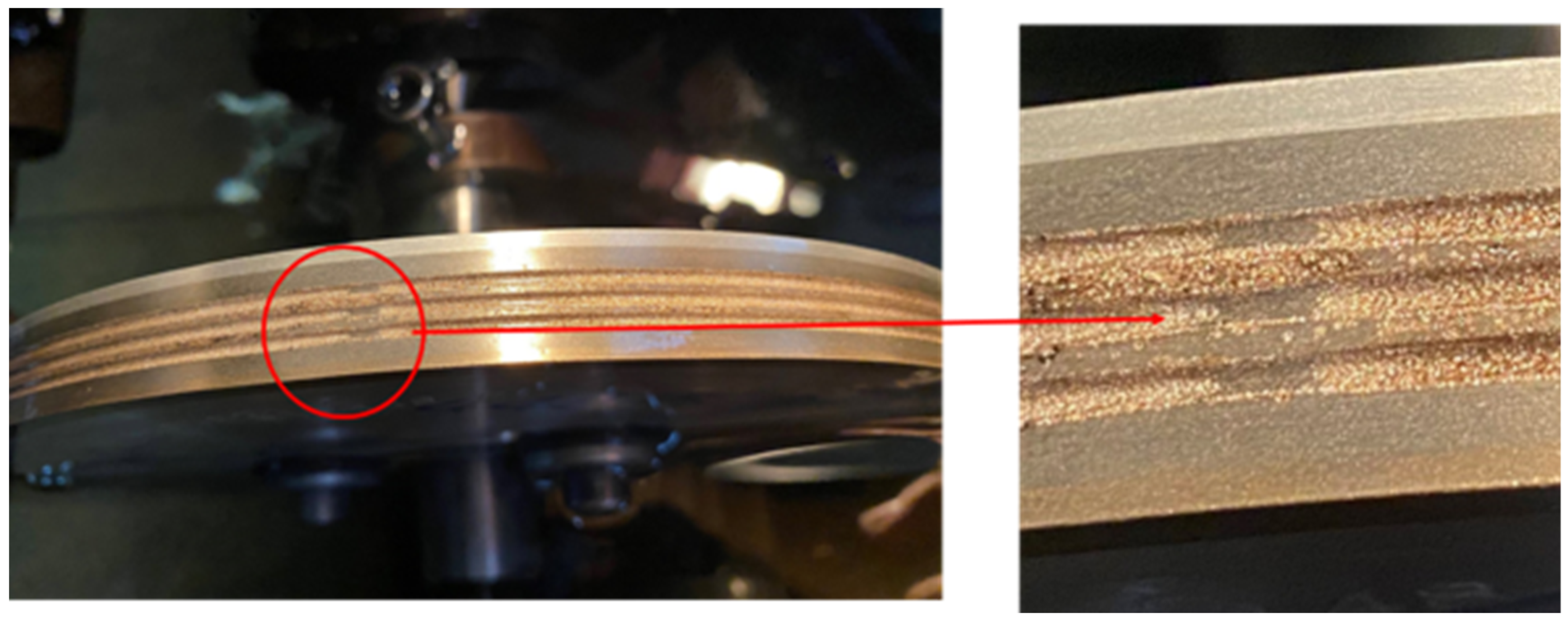
During the processing, if the PCD arrangement is irregular, the large-scale distribution of diamond grit is uneven, as shown in Figure 2. Obvious abnormalities will occur. Not only will the processing produce large friction and impact and the machine vibrate significantly, but also due to the inability to monitor the machine at any time it takes more time to repair and measure when the problem is found. Therefore, the accuracy of the finished product often fails to meet the requirements.

In order to detect the processing process, Caggiano et al. [6] proposed a model-engraving electrical discharge machining monitoring to achieve zero-defect manufacturing. To find out the correlation between processing parameters and inappropriate processing conditions, the model was established with eight highly correlated parameters and monitored with a sampling interval of 32 milliseconds. Caggianoa et al. [7] used a sensor to collect voltage and current signals at a high sampling rate to find ten most relevant features of electrical discharge machining. However, due to the long processing time and the huge amount of data, Gan et al. [8] proposed to use data mining algorithms to solve the feature dimension problem. They reduced the dimension through feature selection models and supervised learning methods, using a self-paced regularizer and ℓ_2,1-norm control model.

Proposed to study the sensors and EDM and established a linear regression model with current and pulse time to predict the surface roughness of the workpiece, by collecting its voltage and current signals, through effective wave extraction, feature calculation, feature matching, and selection of important features and established a model to estimate machining accuracy [9,10,11].

In the EDM process, Wilfried König (1974) proposed that the heat load in the processing was the main factor. The process was affected by heat, causing the temperature to exceed the melting point and even evaporate. Therefore, the edge area of the workpiece corroded by sparks was divided into a solidified layer and a heat-affected zone. (HAZ) and residued form a stress zone (RSZ) on the workpiece. The thickness of this layer depended on the processing parameters [12].

Anomaly detection is an important topic in many fields, and there are many different solutions. Hodg [13] applied statistics and neural-like machine learning methods, which provided a wide range of sample techniques, and proposed three basic principles of clustering methods (clustering approach), classification approaches (classification approach) and novelty approaches (novelty approach). The timing of use depended on the type of data to determine whether to pre-mark the data so that abnormal values were found to process the data. Francis [14] et al.’s novelty detection system based on neural network method was compared to the feature extraction of the data set. The algorithm had equivalent accuracy.

Aiming at the method of anomaly detection, Zhang et al. [15] analyzed arc welding. First, the pre-processing of the arc spectrum was performed on 50 features, and then a measurement index was proposed based on the mean accuracy. Finally, six features were selected to establish an anomaly recognition model based on random forest [16,17]. Chen [18] proposed the limit gradient enhancement method (XGBoost), which was a scalable enhancement system. Through additive training, the current model was retained for each training and a new function is added to the model. Enhancement of the basis was beneficial to the improvement of the objective function.

Characteristics of electrical discharge machining: as the phenomena changes in electrical discharge machining are affected by the relationship between voltage and current [1], the machining accuracy can be estimated with this index [2,11]. Previous research analysis steps and methods [11,12] found the key trend of abnormal electrical discharge machining.

Suitable for single-machine monitoring architecture: due to the difference in processing characteristics between machines, the threshold or model needs to be adjusted. Otherwise it is only suitable for a single machine [12]. After finding the key features, the multiple of steps to monitoring is more convenient and can be presented instantly.

Anomaly detection method: the main reasons for the abnormality of electrical discharge machining are thermal influence and processing parameters [14], the application of statistical methods [15] to detection, even similar neural networks, random forests [16], and XGB-RF. In order to achieve heir goal, more effective use of multiple models could make the results more reliable. Chakraborty [19] developed a model using XGBoost. Their method involves dynamically adjusting thresholds based on predicted real-time moving averages and moving standard deviations to quickly detect faults in HVAC systems.

Therefore, this research further develops an electrical discharge machining real-time monitoring system. Through feature analysis and model diagnosis, it has been able to identify abnormal phenomena at a high level. The specific contributions are as follows:

Abnormal characteristics of electrical discharge machining: the newly-added coefficient of variation feature effectively reduces the amount of macro data, and uses KLD (Kullback–Leibler divergence) as an indicator to calculate the change in processing per minute, so that abnormal processing can now be analyzed.

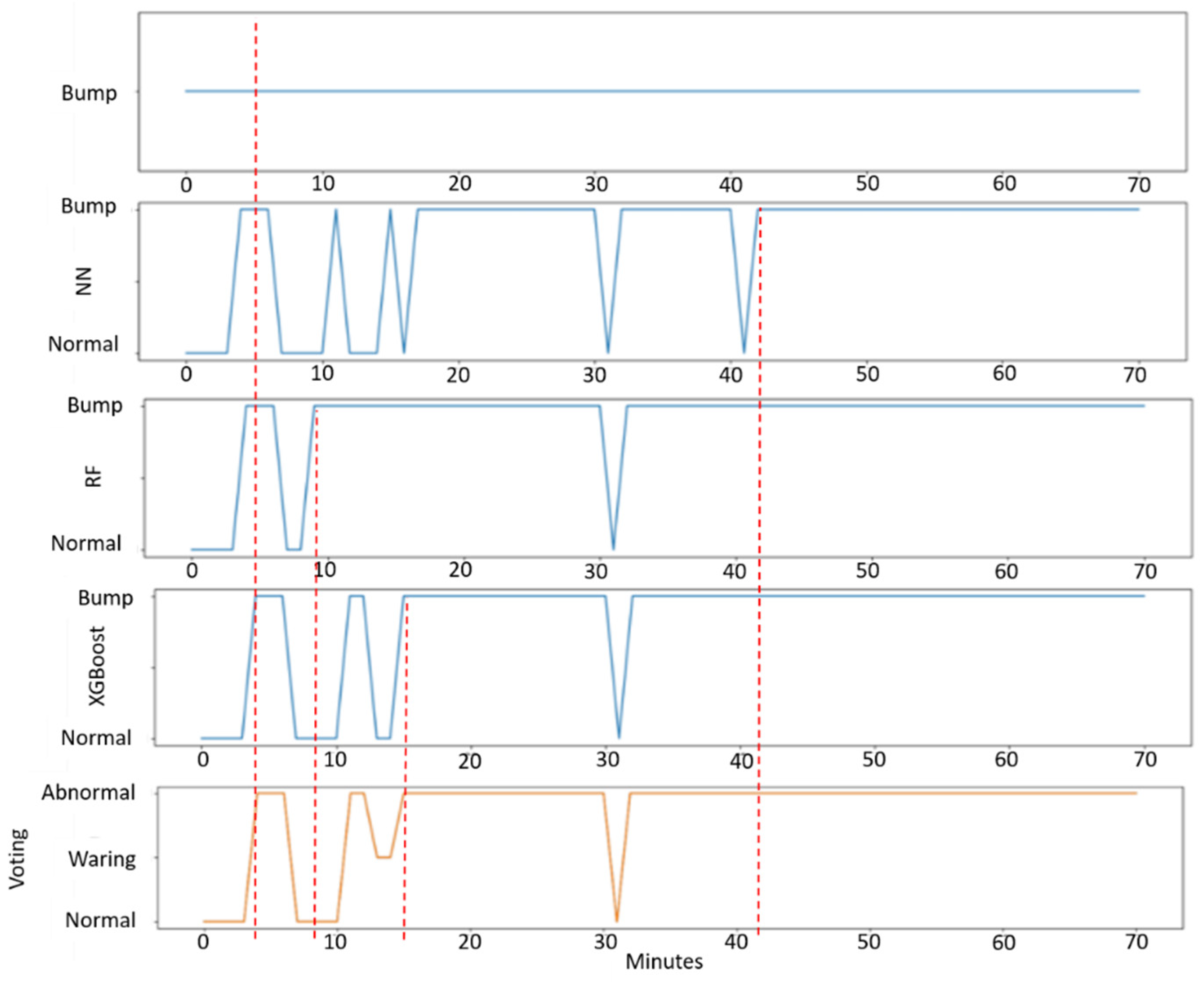
Discharge machining anomaly detection methods of our proposed study are carried out on the basis of three methods (neural network, random forest, and XGB-RF), which are models established separately to identify abnormal processing. Finally, we used voting rules to reduce the weight of a single model and identify false alarms.

2. Proposed Methodology

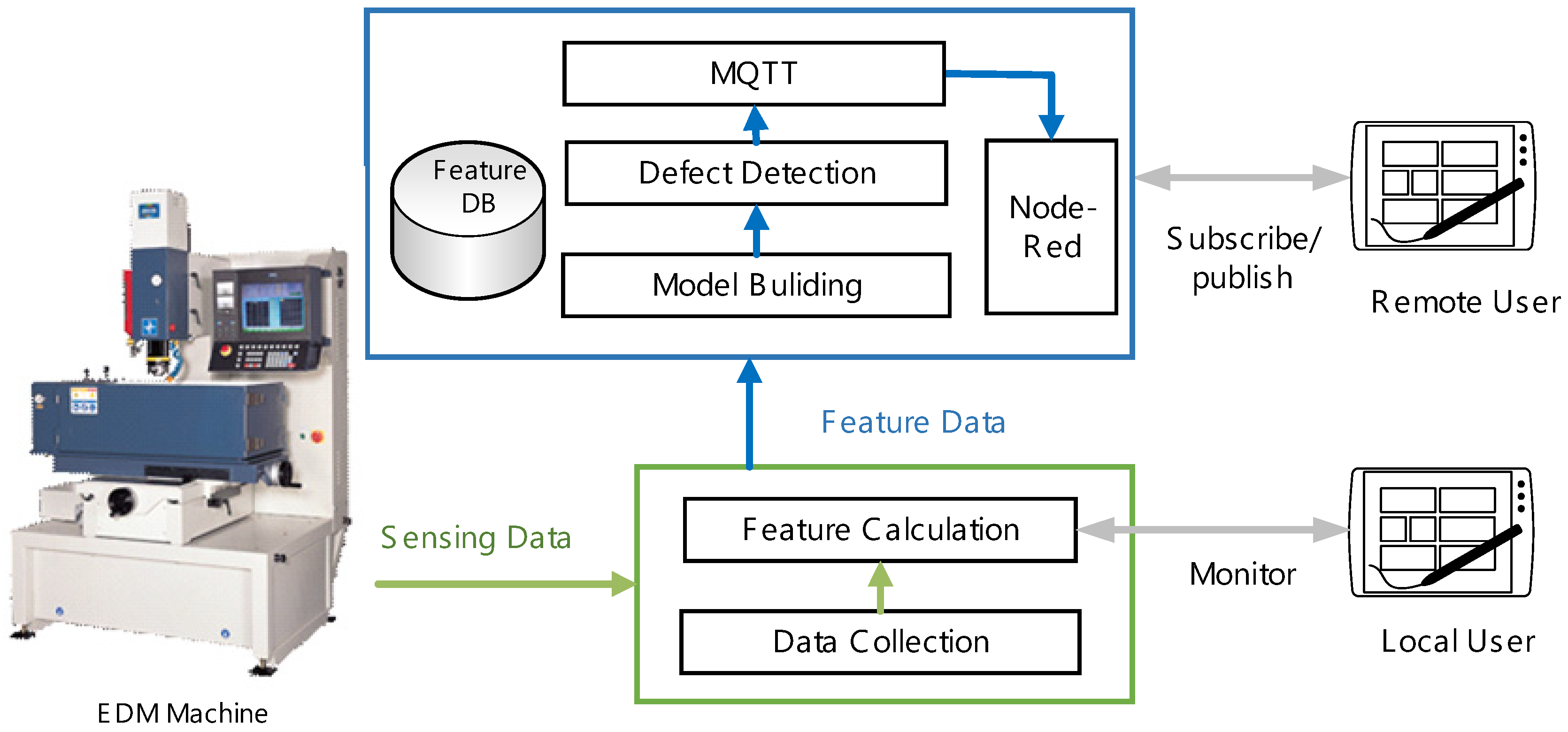
The methodology of our proposed system will focus on EDM abnormal monitoring based on the collected raw data of the EDM machine by retrieving the pulse voltage and current as input data. The defect detection model of EDM was constructed by feature data, which were obtained and picked through the data collection and feature calculation. The output of our proposed system would indicate the status of EDM machine and process quality. The processing flow of the EDM abnormal monitoring system is shown in Figure 3. A high-voltage probe and a current check meter are installed on the processing machine. While starting the machining process, the characteristic calculation would synchronously be to perform based on the retrieving pulse voltage and current data. After obtaining the characteristics, it will be divided into storage and data exchange. The stored data are a log file, and the exchanged data will enter the model analysis. Models are established separately based on characteristics and anomaly monitoring methods, and then decisions are made by voting methods. An abnormality detection system is developed for electrical discharge machining, and transmitting its information to Node-RED via the MQTT (message queuing telemetry transport) communication protocol, which can provide real-time monitoring of machine abnormalities and display the current status of machining.

2.1. Feature Calculation Method

Electric discharge machining melts the workpiece through spark discharge to achieve the purpose of material removal. In the discharge process, the process indicators of peak current, peak voltage, discharge cycle time, discharge gap, etc. change over time. The key characteristics will be calculated, which can be defined as follows:

a.

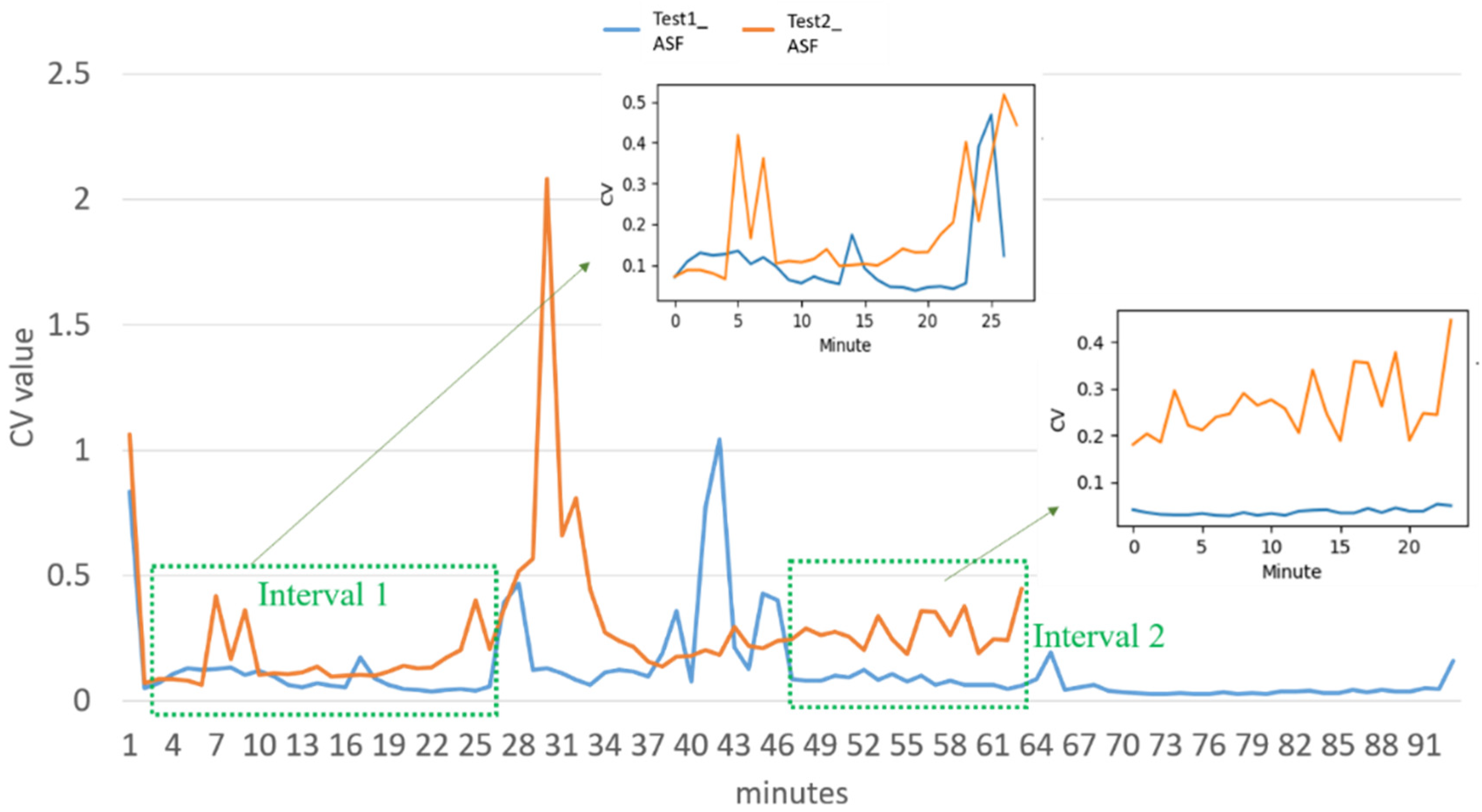
Average spark frequency (ASF)

Spark is defined as when the electrode (positive electrode) almost touches the workpiece (negative electrode) during the machining process, when the electrode is charged and discharged, a current loop will be formed between the electrode and the workpiece, and the current will rise and continue until the end of the discharge. The process is called a spark. The spark frequency is defined as the total number of sparks N_t generated within a period of time T_t, as shown in Equation (1):

$$\mathrm{ASF}=\frac{{\mathrm{N}}_{\mathrm{t}}}{T_{\mathrm{t}}}$$

(1)

b.

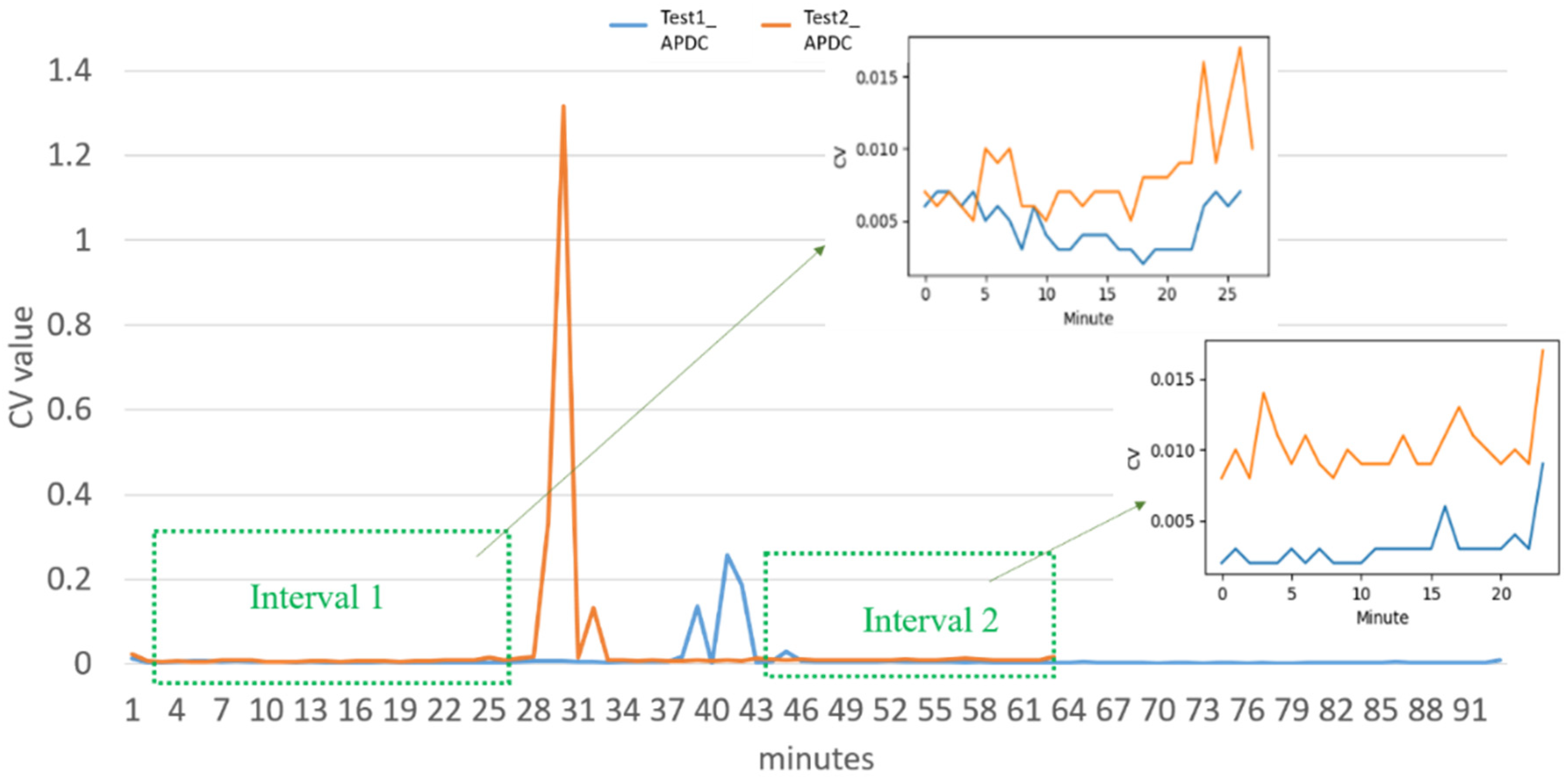
Average peak discharge current (APDC)

When the i-th spark is generated in the discharge process, the maximum current I_i(max) existing is defined as the discharge peak current. The average discharge peak current when all sparks are generated is the average discharge peak current, as shown in Equation (2):

$$\mathrm{APDC}=\frac{1}{{\mathrm{N}}_{\mathrm{t}}}{\displaystyle \sum }_{i=1}^{{\mathrm{N}}_{\mathrm{t}}}{\mathrm{I}}_{i\left(\max \right)}$$

(2)

c.

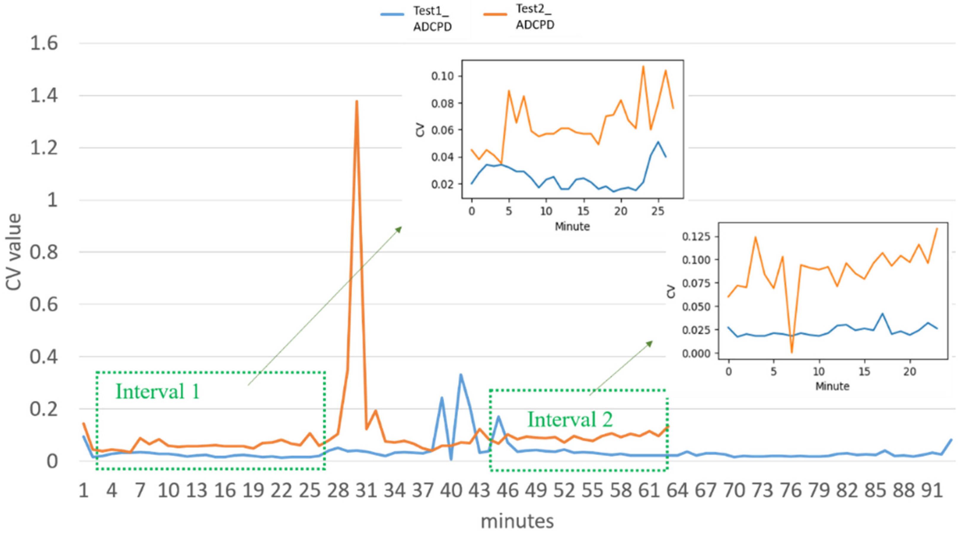
Average discharge current pulse duration (ADCPD)

When Δt_i period is from the beginning to the end of the i-th spark generation. T_t is defined as the discharge current pulse duration. N_t is defined as the discharge current pulse duration. The average discharge current pulse duration is the average of all spark times, as shown in Equation (3):

$$\mathrm{ADCPD}=\frac{1}{{\mathrm{N}}_{\mathrm{t}}}{\displaystyle \sum }_{i=1}^{{\mathrm{N}}_{\mathrm{t}}}\mathsf{\Delta }{\mathrm{t}}_i$$

(3)

d.

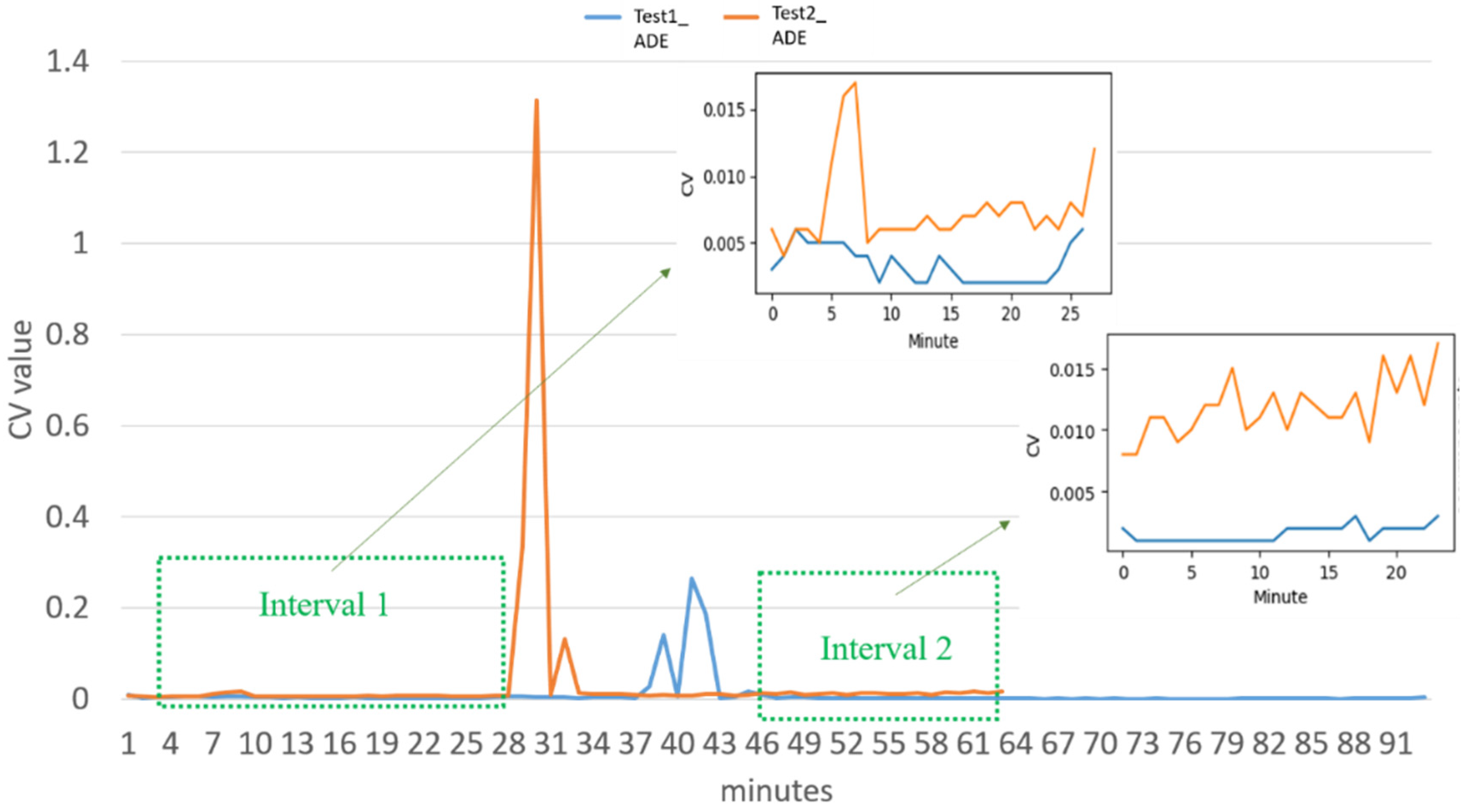
Average discharge energy, ADE

In the spark discharge process, the actual voltage and current are variable values, as well as the i-th discharge energy (E_i). Formula is shown in Equation (4):

$$\mathrm{ADE}=\frac{1}{{\mathrm{N}}_{\mathrm{t}}}{\displaystyle \sum }_{i=1}^{{\mathrm{N}}_{\mathrm{t}}}{\mathrm{E}}_i$$

(4)

where ${\mathrm{E}}_i={{\displaystyle \int }}_0^{T_{\mathrm{t}}}{\mathrm{I}}_{\mathrm{t}}{\mathrm{V}}_{\mathrm{t}}\mathrm{dt}$, V_t is discharge voltage and I_t is the discharge current.

e.

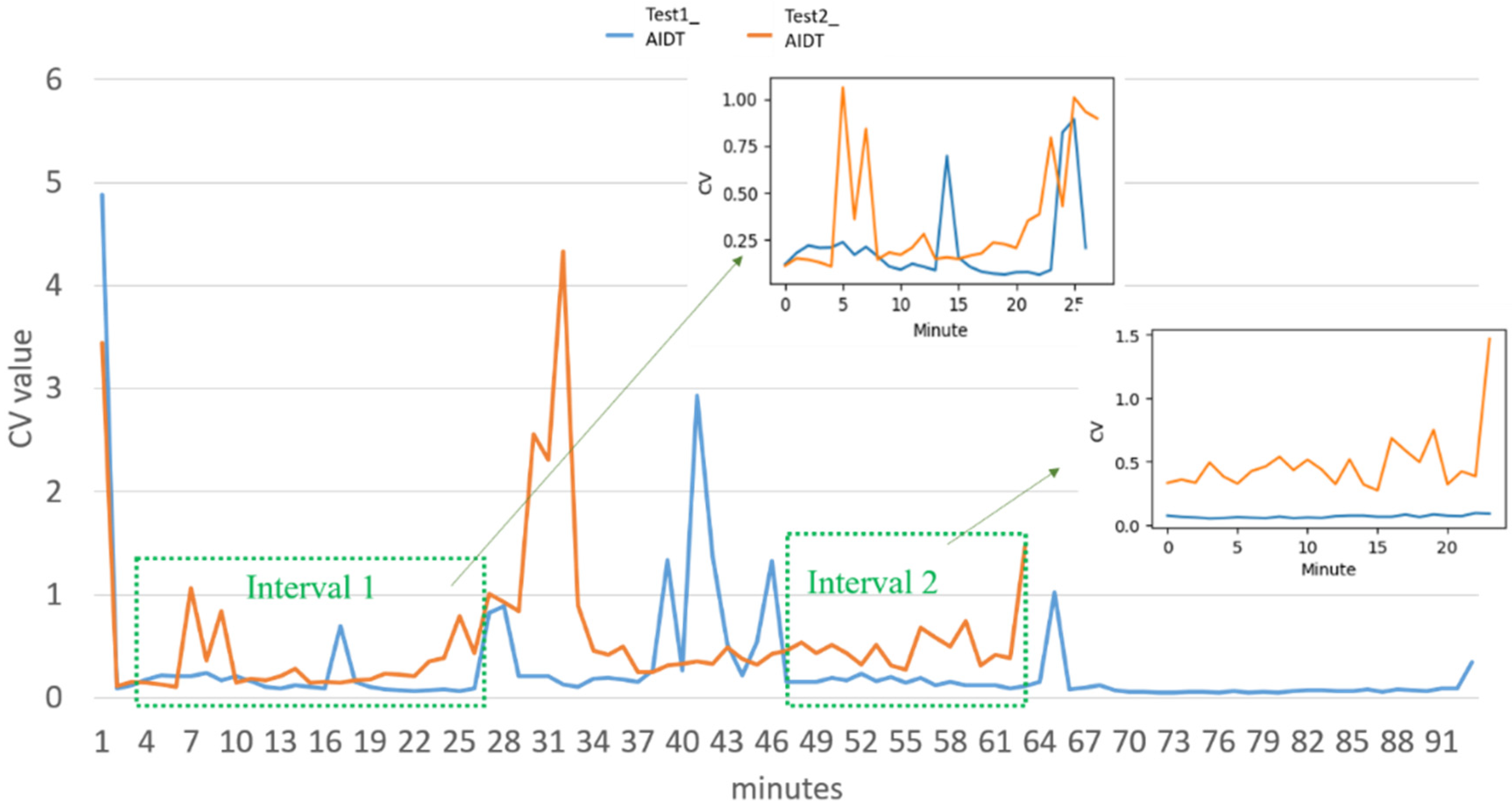
Average ignition delay time, AIDT

In the i-th discharge, the open circuit voltage time t_d,i and the effective discharge current time t_e,i are defined as the ignition delay time. The average ignition delay time is the average of all ignition delay times, as shown in Equation (5):

$$\mathrm{AIDT}=\frac{1}{{\mathrm{N}}_{\mathrm{t}}}{\displaystyle \sum }_{\mathrm{i}=1}^{{\mathrm{N}}_{\mathrm{t}}}\left({\mathrm{t}}_{\mathrm{e},i}-{\mathrm{t}}_{\mathrm{d},i}\right)$$

(5)

f.

Average gap voltage, AGV

When the open circuit voltage of the i-th discharge reaches the effective discharge current, the maximum voltage V_i(max) generated during this period is defined as the gap voltage. The average of all open-circuit peak voltages are taken to get the average gap voltage, as shown in Equation (6):

$$\mathrm{AGV}=\frac{1}{{\mathrm{N}}_{\mathrm{t}}}{\displaystyle \sum }_{i=1}^{{\mathrm{N}}_{\mathrm{t}}}{\mathrm{V}}_{i\left(\max \right)}$$

(6)

g.

Open circuit ratio, OCR

When the voltage peak ends, discharge is required, but the current peak does not rise and is defined as an open circuit. The open circuit ratio is the total number of open circuits O_t divided by the total number of sparks N_t in a period of time T, as shown in Equation (7):

$$\mathrm{OCR}=\frac{{\mathrm{O}}_{\mathrm{t}}}{{\mathrm{N}}_{\mathrm{t}}}$$

(7)

h.

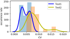
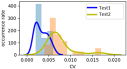
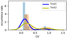
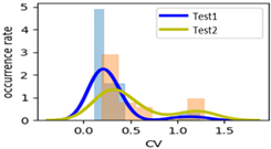
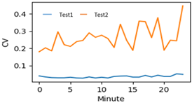
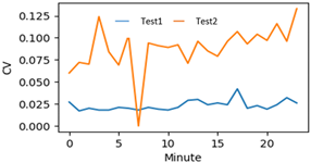
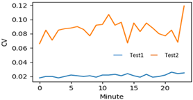
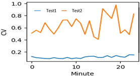
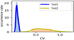
Coefficient of variation, CV

The coefficient of variation of a set of data is defined as the value obtained by dividing the standard deviation σ of this set of data by the mean μ, as shown in Equation (8). The coefficient of variation is the relative amount of difference, which is used to compare the dispersion of the two sets of data.

$$\mathrm{C}.\mathrm{V}.=\frac{\mathsf{\sigma }}{\mathsf{\mu }}$$

(8)

2.2. Anomaly Detection Method

i.

Neural network

In order to evaluate the nonlinear relationship between input and output, neural networks (NN) with supervised learning artificial neural networks have proven their effectiveness in many fields. NN is composed of multiple nodes, where X = [x₁, …, x_n] is the input vector, W = [w₁, …, w_n] is the weight of each input, and b is the partial weight, which is a kind of neural network algorithm modification input value. The activation function f equation is then inputted and the result y is outputted. The overall neural network algorithm is expressed by the equation as shown in Equation (9):

$$\mathrm{y}=\mathrm{f}\left(\mathrm{WX}+\mathrm{b}\right)$$

(9)

j.

Random forest

The random forest algorithm is based on statistical theory and is a method of machine learning [20]. Using the algorithm of classification regression tree and bootstrap to resample the original data, new data are then generated, a decision tree for each bootstrap sample is built, and finally the final result is obtained by a voting method with the same weight of the classifier [20]. It can be applied to detection with less abnormal data.

k.

XGBoost

Chen [17] proposed the extreme gradient boosting (XGBoost) method. In order to solve the problem of the accuracy and speed of the decision tree in the face of supervised learning, the traditional decision tree is mainly based on the classification tree, and XGBoost is added to the regression tree. XGBoost can optimize numerical values more effectively, not only reducing overfitting but reducing the amount of calculation. Supervised learning allows machine learning building a model through training data with multiple characteristics, and use the model to predict the result of the target variable. The model is represented by a mathematical function. Given the X variable to predict the target function of the Y variable, the parameters of the model will be continuously learned and adjusted from the data. In addition, the problem type can be determined according to the difference in the predicted value of the target function. Divided into regression or classification. General classification models are based on linear development, y_i is the predicted value of sample x_i, k is the total number of decision trees, and w_k is the weight of the k-th number, as shown in Equation (10):

$$\widehat{y_i}={\displaystyle \sum }_{k=1}^k{w}_k{x}_{ik}$$

(10)

The target function of XGBoost uses l as the loss function to measure the difference between $\widehat{y_i}$and y, and Ω is the regularization term, which contains two parts. The first is 𝛾𝑇 and the second, T, is the decision tree. For the nodes above, 𝛾 is the hyper parameter. If 𝛾 is larger, the node will be smaller. The other part is adjusted by the weight of the child nodes to avoid overfitting. ω is the weight of the child nodes, as shown in Equations (11) and (12):

$$Obj(\varnothing )={{\displaystyle \sum }}_{i}l\left({\widehat{y}}_i,y\right)+{{\displaystyle \sum }}_k\mathsf{\Omega }\left(f_k\right)$$

(11)

$$\mathsf{\Omega }\left(f\right)=\mathsf{\gamma }T+\frac{1}{2}\lambda {||\omega ||}^2$$

(12)

l.

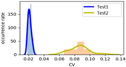
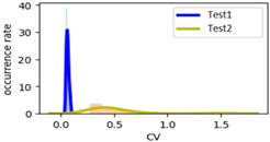
KL divergence

Kullback-Leibler Divergence, KLD, also known as relative entropy, is used to measure the divergence difference of two probability distributions in the same spatial event, which is the difference between the probability distribution p(x) and the arbitrary probability distribution q(x). The probability distributions P and Q of continuous random variables are defined as KL(P||Q) as shown in Equation (13):

$$\mathrm{KL}(\mathrm{P}||\mathrm{Q})={\displaystyle \int }p\left(x\right)\log (\frac{p\left(x\right)}{q\left(x\right)})dx$$

(13)

When the value of KL(P||Q) is smaller, it means that the probability distribution of P and Q is more similar. On the contrary, the larger the value, the greater the difference between the two probability distributions. If p(x) = q(x), KL (P||Q) is zero, KL(P||Q) can be used to calculate the difference between the two probability distributions.

m.

Confusion matrix

The confusion matrix is meant to test the capabilities of the model. A model built from training data is inputted into the model. The model will calculate each datum, and the model results and actual conditions will generate a result analysis table. There are four conditions:

TP (true positive): the actual state is normal, and the model judges it to be normal.

FP (false positive): the actual state is abnormal, and the model judges it to be normal.

FN (false negative): the actual state is normal, and the model judges it to be abnormal.

TN (true negative): the actual state is abnormal, and the model judges it to be abnormal.

The sensitivity, specificity, false positive rate (Fpr), and false negative rate (Fnr) of the model based on the four conditions are calculated, as shown in Equations (14)–(17).

$$\mathrm{Sensitivity}=\frac{\mathrm{TP}}{\mathrm{TP}+\mathrm{FN}}$$

(14)

$$\mathrm{Specificity}=\frac{\mathrm{FN}}{\mathrm{FP}+\mathrm{TN}}$$

(15)

$$\mathrm{Fpr}=1-\mathrm{Sensitivity}$$

(16)

$$\mathrm{Fnr}=1-\mathrm{Specificity}$$

(17)

The higher the sensitivity result, the higher the accuracy rate of the normal processing state model judgement. Otherwise, the higher the result, the lower the missed detection rate (which is ideally zero). The higher the specific result, the higher the abnormal processing state model judgement accuracy rate. On the contrary, the false positive rate will be lower (the ideal is zero).

3. Case Study

3.1. Experimental Results of Feature Calculation

This diagnostic recording experiments on the actual launch processing machine will be conducted. Aiming at the high points caused by uneven distribution of diamond particles, the processing experiments and analysis are conducted.

After calculating the seven features, the coefficient of variation of each feature per minute is calculated. Taking 26 min (1–25 min) before abnormal processing as the normal value and 23 min (40–63 min) after processing as interval 2, interval 1 and interval 2 are converted into probability, and the KLD value of the two intervals is calculated. It has occurred, and the time when it appears with probability is not obvious. In a period of time, the second period is significantly shorter. KLD increases by 0.209. The abnormal method can determine the normal and processing trends shown in Figure 4.

In the average spark frequency (ASF), the KLD value of interval 1 is 3.097, and the KLD value of interval 2 is 4.236. In this feature, the KLD value of both intervals is greater than 3, indicating that there is a clear trend of positive and abnormal machining in two intervals, especially in interval 2, the distribution of normal processing is almost concentrated in the range of 0.05 to 0.15, while the distribution of abnormal processing is in the range of 0.2 to 0.4, shown in Figure 5.

In the average energy (ADE), the KLD value of interval 1 is 4.128 and the KLD value of interval 2 is 1.476. This feature is as high as 4 in interval one, indicating that the coefficient of variation of normal processing energy is relatively concentrated (0.002–0.004), while abnormal processing energy variation coefficient is relatively scattered (0.004–0.016), which makes the distance elongated. The KLD value is therefore very large, meaning that normal and abnormal processing trends can be observed in the first interval, shown in Figure 6.

In the average discharge current pulse duration (ADCPD), the KLD value of interval 1 is 0.889. The KLD value of interval 2 is 0.864, and the KLD value of both intervals is less than 1. Although the difference can be seen in the distribution, the distribution value is only between 0.02 and 0.1, shown in Figure 7.

In the average gap voltage (AGV), the KLD value of interval 1 is 2.617, the KLD value of interval 2 is 3.16, and the KLD values of both intervals are greater than 2.5, indicating that normal and abnormal processing can be distinguished, especially in interval 2, where the two distributions are clearly separated, shown in Figure 8.

In the average gap voltage (AGV), the KLD value of the interval 1 is 0.124, the KLD value of the interval 2 is 1.419, and the KLD value of the interval 2 is 1.295 larger than that of the interval, shown in Figure 9.

In the open circuit ratio (OCR), the KLD value of interval 1 is 2.844, the KLD value of interval 2 is 1554, the distribution of abnormal processing in interval 1 is more concentrated in 0–0.4, and the distribution of normal processing in interval 2 is more concentrated in 0–0.5. This means that the two processing abnormal behaviors are different, although they can still be classified, shown in Figure 10.

3.2. Model Judgment Result

The summary of exponential results for interval 1, shown in

Table 1. Results for interval 1.

Characteristic	Raw Data	CV
APDC
ASF
ADE
ADCPD
AGV
AIDT
OCR

.

The summary of exponential results for interval 2, shown in

Table 2. Results for interval 2.

Characteristic	Raw Data	CV
APDC
ASF
ADE
ADCPD
AGV
AIDT
OCR

.

In this section, abnormal processing is used as the verification, and the models trained with the features in Section 3.1 are input, respectively. In order to avoid misjudgment caused by a single method, three independent models are trained in three methods (respectively, NN, RF, and XGB-RF), and the voting rules are used for reducing the problem of excessive weight for a single model.

The experimental results significantly indicated that the CV values of these seven features (e.g., ASF, ADE, etc.) were obviously separated into two clusters between the normal and abnormal machining processes. The EDM abnormal monitoring model was trained well by picking up the key features of the raw data. In order to avoid misjudgment caused by a single method, three independent models were adopted to be trained in three independent methods (NN, RF, and XGB-RF, respectively). The voting rules reduce the problem of excessive weight for a single model. In summary, three models indicated either a normal or abnormal case forward equal response. Only single model voting would lead to pre-warning (and not a warning state of the EDM machine).

In the model judgment result, as shown in Figure 11, after the 16th minute of the NN model, the judgment result begins to stabilize, and the judgment only misses for 2 min in the subsequent 55 min. After 8 min of the RF model, the judgment result begins to stabilize, and within 63 min, only 1 min is missed. The XGB-RF model starts to stabilize after 14 min, and within 57 min, only 1 min is missed. With the voting mechanism added, as a whole, the sensitivity can reach 0.974 and the Fpr is 0.07. Compared with the previous two seconds, it is judged formally. The sensitivity reaches 0.93 and the Fpr is 0.002.

4. Conclusions

Our proposed research would focus on the pre-diagnosis and in-line monitoring which is applied for the EDM process. The seven key characteristics of the process would lead us to know the quality of the machining process. The abnormality of electrical discharge machining could be easily recognized based on the above-mentioned key characteristics. This research adds a coefficient of variation and provides a feature analysis in real-time. The model of the neural network and random forest and XGB-RF methods were adopted for anomaly detection. The three results are equally emphasized by voting rules and then formally judged as anomalies in the most cautious way. The accuracy of our prediction model can approach 0.93, and the false positive rate is only 0.002. According to our proposed configuration, the system is no longer limited to different machines. In order to reduce the trouble of false alarms, the formal judgment should be based on two consecutive model results.