Article

Calculation of the Insertion Loss of Barriers on Rigid Ground in the Time Domain

Key Laboratory of Modern Acoustics, Institute of Acoustics, Nanjing University, Nanjing 210093, China
*
Authors to whom correspondence should be addressed.
Appl. Sci. 2022, 12(4), 2018; https://doi.org/10.3390/app12042018
Submission received: 20 January 2022 / Revised: 12 February 2022 / Accepted: 14 February 2022 / Published: 15 February 2022
(This article belongs to the Special Issue Sound Field Control)

Abstract

:
This paper presents a method for calculating the insertion loss of barriers on the ground. The method combines the classic imaging method for an analysis of sound propagation with the secondary source model for diffraction by barriers in the time domain, which is different from other frequency-domain methods. The validity of the proposed method is verified by comparing the theoretical results with those derived from the MacDonald method, and a valid approximation for the infinite barrier is discussed.

1. Introduction

Sound barriers have been widely used for noise reduction in daily life, such as roads [1] and buildings [2]. Sound barrier research essentially can boil down to the diffraction problem. Hence, to better improve the acoustic performance of noise barriers, it is important to accurately calculate the sound field diffracted by barriers.
Since the 19th century, many studies have been carried out on sound diffraction by barriers. In 1896, Sommerfeld [3] first presented a mathematically rigorous solution for the diffraction problem of a plane wave and a cylindrical wave incident on a thin rigid half plane. Carslaw [4] and MacDonald [5] extended Sommerfeld’s method to the spherical incident case. Hadden and Pierce [6] developed an analytical model for wedge diffraction based on Green’s function and used the Laguerre technique for numerical integration. Zhao et al. [7] proposed an analytical method for calculating a sound field based on the integral equation method. Then, Huang et al. [8] extended this method to investigating the effects of top edge impedance on sound barrier diffraction.
Besides the frequency-domain analytical solutions above, time-domain solutions for diffraction have also been developed. Biot and Tolstoy [9] provided a closed-form time-domain solution for the impulse response of an infinite rigid wedge. Medwin et al. [10] proposed a discrete Huygens interpretation to model diffraction using a finite wedge by assuming the existence of secondary edge sources located along the apex of the wedge. Svensson et al. [11,12] extended this model by deriving analytical directivity functions for the secondary edge sources.
In addition to the solutions above, the geometrical theory of diffraction (GTD) [13], the uniform geometrical theory of diffraction (UTD) [14], and the physical theory of diffraction (PTD) [15] are widely used diffraction theories. Moreover, the classic boundary element method (BEM) [16,17,18] and the finite element method (FEM) [19,20,21] have found application in the calculation of barrier diffraction.
It is worth noting that most of the studies above neglected the effect of ground reflections. L’Esperance et al. [22] combined the Hadden–Pierce solution with the imaging method to study the insertion loss of absorbent barriers on the ground. Buret [23] utilized a semi-empirical model to investigate the dipole sound field diffracted by a barrier above an impedance ground. Zhao et al. [24] developed an integral equation method for calculating diffraction using a rigid barrier on the ground. However, most of these methods focused on the frequency domain and rarely adopted time-domain solutions to address ground reflections. It is convenient to perform a method in the time domain as it handles the whole frequency range at the same time due to the time-domain nature, while frequency-domain methods have to repeat the process point by point in the range of interest. Moreover, this is a basis for future extension of this method to a moving sound source.
This paper combines the time-domain Svensson method [11,12] of wedge diffraction with the image method to investigate the insertion loss of a rigid barrier on a rigid ground. The validity of the proposed method was verified by comparing the theoretical results with those derived from the MacDonald method, which has been verified by experiments and other methods [7,24]. A valid approximate substitution for the infinite barrier was discussed.

2. Theory

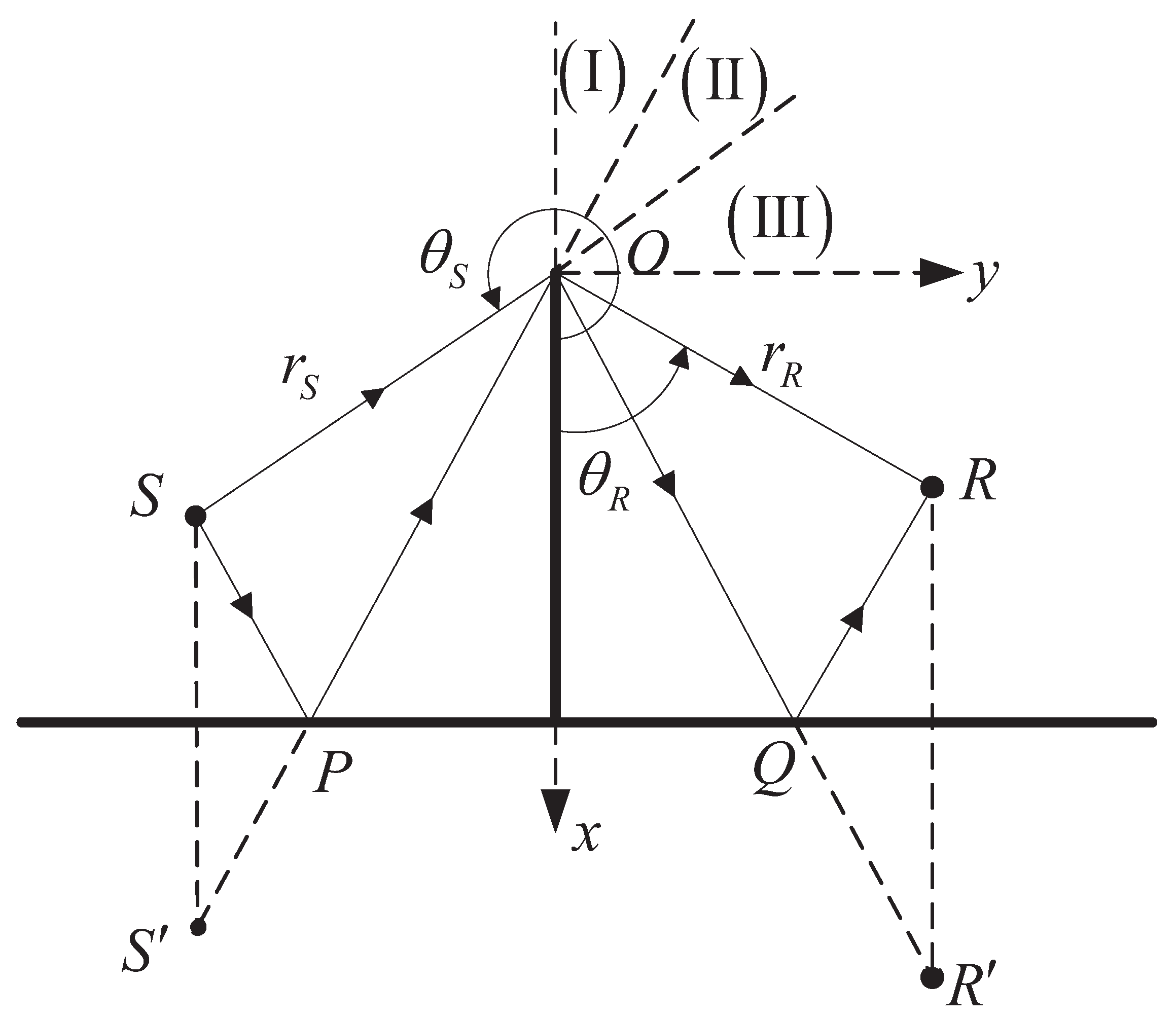
2.1. The Secondary Edge Source Model

Figure 1 shows the geometry of a rigid wedge and cylindrical coordinate system. The source signal is defined as q ( t ) = ρ A ( t ) / 4 π so that the free-field impulse response of the source is h S ( t ) = δ ( t d / c ) / d , where ρ is the density of air, A ( t ) is the volume acceleration of the point source, c is the speed of sound in air, and d is the source-to-receiver distance. Following Svensson et al. [11,12], the sound field diffracted by a wedge can be described as
p D S R ( t ) = ν 4 π z 1 z 2 q ( t m + l c ) β m l d z ,
where z 1 and z 2 are the two endpoints of the finite or infinite wedge; ν = π / θ W is the wedge index; θ W is the exterior wedge angle; and m and l are distances from the edge point z to the source S ( r S , θ S , z S ) and receiver R ( r R , θ R , z R ) , respectively. The function β is described as
β ( t ) = β + + ( t ) + β + ( t ) + β + ( t ) + β ( t ) ,
with individual terms defined by
β ± ± ( t ) = s i n [ ν ( π ± θ S ± θ R ) ] c o s h [ ν η ( t ) ] c o s [ ν ( π ± θ S ± θ R ) ] ,
where
η ( t ) = c o s h 1 c 2 t 2 [ r S 2 + r R 2 + ( z S z R ) 2 ] 2 r S r R .

2.2. Estimation of the Insertion Loss via the Image Method
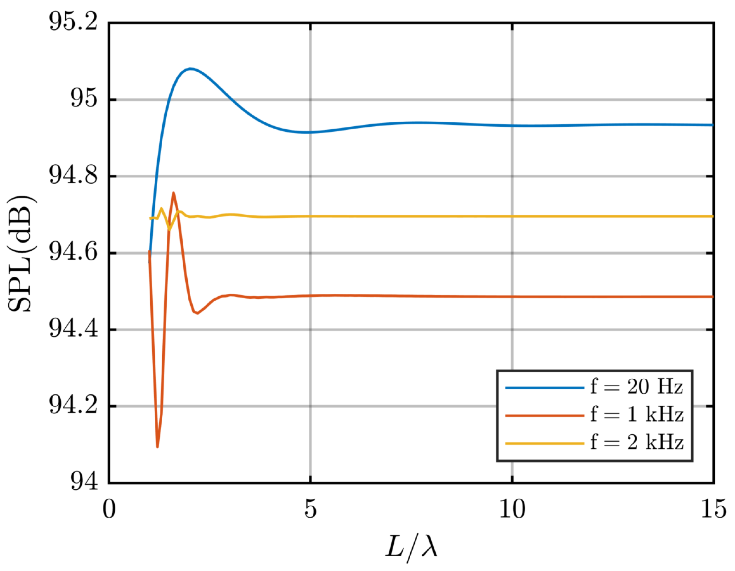
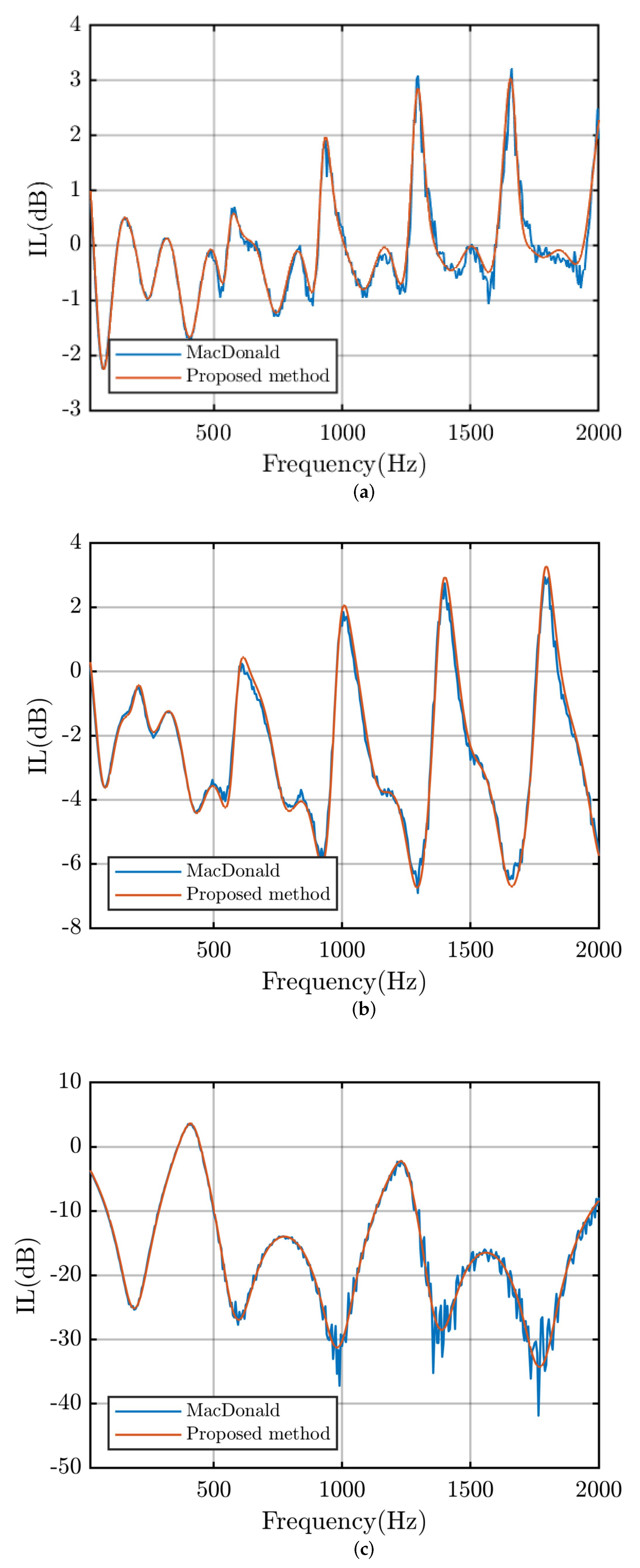
Figure 2 shows the schematic diagram and coordinate systems. Consider sound propagation in the presence of a barrier when the source S ( x S , y S , z S ) and receiver R ( x R , y R , z R ) are located on either side of the barrier above a rigid ground. The barrier is assumed to be infinitely thin, corresponding to θ W = 2 π and located at y = 0 , 0 x h , where h is the height of the barrier and the ground is represented by x = h . The diffracted sound field p D ( t ) at the receiver from the source is a superposition of four components corresponding to four different paths, considering the effect of ground reflections. Thus,
p D ( t ) = p D S R ( t ) + p D S R ( t ) + p D S R ( t ) + p D S R ( t ) ,
where the superscripts represent the four propagation paths related to the source S; the receiver R; the image source S ( x S , y S , z S ) ; and the image receiver R ( x R , y R , z R ) , with x S = 2 h x S and x R = 2 h x R . Then, the cylindrical coordinates of the four positions are as follows:
r S = x S 2 + y S 2 θ S = 2 π c o s 1 x S r S , z S = z S
r R = x R 2 + y R 2 θ R = c o s 1 x R r R , z R = z R
r R = x R 2 + y R 2 θ R = c o s 1 x R r R . z R = z R
According to the sound field components, the space on the right side of the barrier is divided into three regions, as follows:
Region I:
p T ( t ) = p d ( t ) + p r ( t ) + p D ( t ) ,
Region II:
p T ( t ) = p d ( t ) + p D ( t ) ,
Region III:
p T ( t ) = p D ( t ) ,
where p T ( t ) , p d ( t ) , and p r ( t ) represent the total sound field, the direct wave, and the reflected wave, respectively. Thus,
p d ( t ) = ρ 4 π d S R A ( t d S R / c ) ,
p r ( t ) = ρ 4 π d S R A ( t d S R / c ) ,
where d S R and d S R are the distances from the source S and image source S to the receiver R.
The insertion loss of a barrier describes the difference in the sound level with and without the barrier in the presence of the ground in both cases. Thus,
I L = 20 log | p T ( ω ) p g ( ω ) | ,
where p T ( ω ) and p g ( ω ) are the frequency spectra of p T ( t ) and p g ( t ) , respectively. The total sound field p g ( t ) without the barrier can be expressed as
p g ( t ) = p g d ( t ) + p r ( t ) .

3. Simulation

It is efficient and acceptable to approximate the infinite barrier with a finite one, as proved in Figure 3. For better comparison, the sound pressure level (SPL) for frequencies f = 1 kHz and f = 2 kHz in Figure 3 are artificially raised to 28 dB and 14.5 dB, respectively. The sound pressure level at the receiving point R 3 ( 0.5 , 0.5 , 0 ) m from the source S ( 0.5 , 0.5 , 0 ) m converges with the ratio L / λ , where L is the length of the barrier and λ is the wavelength. Lower frequencies require longer barriers. When the barrier length L increases to 10 λ , the convergence is sufficient for the whole frequency range. Thus, the barrier length L is set to 20 m, with its middle edge point located at the origin O of the coordinate systems in the following simulations using MATLAB. The barrier has a height of 1 m.
To check the validity of the method described in the previous section, the results are compared with those derived from the MacDonald method. Three receiving points corresponding to regions I, II, and III are selected as R 1 ( 0.6 , 0.1 , 0 ) m , R 2 ( 0.3 , 0.2 , 0 ) m and R 3 . Figure 4 presents the insertion loss at three different receivers from the same source. The time-domain method agrees reasonably well with the MacDonald method in the frequency range of interest in different regions. The Mean Absolute Error (MAE) values corresponding to the three receiving positions R 1 , R 2 , and R 3 in Figure 4 are 0.1, 0.2, and 0.8, respectively. Moreover, the calculation with the proposed method is more efficient compared with the MacDonald method. The frequency-domain MacDonald method take 78 s to calculate 397 frequency points using a computer with 1.60 GHz main frequency and 16 GB random access memory. By contrast, the proposed method takes 3 s for the whole frequency range as it operates in the time domain with a sampling frequency of 48 kHz.

4. Conclusions

In this paper, an analytical method for calculating the insertion loss of barriers on the ground was described. In line with the theory, the time-domain method for wedge diffraction proposed by Svensson et al. was combined with the classic image method for the analysis of sound propagation over a barrier on the ground. The accuracy of the proposed method was validated using the classic MacDonald method. Moreover, the proposed method has faster processing speed than the conventional MacDonald method. In addition, the proposed method can calculate the whole frequency range at the same time due to the nature of the time domain, while frequency-domain methods have to repeat the process point by point in the range of interest. However, the proposed method is currently restricted more by the fact that it does not allow for absorbent barriers and impedance ground. Thus, our future work will focus on an extension of our method to absorbent barriers and finite impedance ground. Moreover, predictions of a finite barrier or moving source effects would be interesting.

Author Contributions

Conceptualization, J.G.; methodology, J.G.; software, J.G. and X.F.; validation, J.G.; formal analysis, J.G.; investigation, J.G.; resources, J.G. and Y.S.; data curation, J.G.; writing—original draft preparation, J.G.; writing—review and editing, J.G., X.F. and Y.S.; visualization, J.G.; supervision, X.F. and Y.S.; project administration, X.F. and Y.S. All authors have read and agreed to the published version of the manuscript.

Funding

This research received no external funding.

Institutional Review Board Statement

Not applicable.

Informed Consent Statement

Not applicable.

Data Availability Statement

Not applicable.

Conflicts of Interest

The authors declare no conflict of interest.

References

  1. Pardo-Quiles, D.; Rodríguez, J.V.; Molina-García-Pardo, J.M.; Juan-Llácer, L. Traffic Noise Mitigation Using Single and Double Barrier Caps of Different Shapes for an Extended Frequency Range. Appl. Sci. 2020, 10, 5746. [Google Scholar] [CrossRef]
  2. Tang, S.K. Noise screening effects of balconies on a building facade. J. Acoust. Soc. Am. 2005, 118, 213–221. [Google Scholar] [CrossRef] [PubMed]
  3. Sommerfeld, A. Mathematische Theorie der Diffraction. Math. Ann. 1896, 47, 317–374. [Google Scholar] [CrossRef]
  4. Carslaw, H.S. Diffraction of Waves by a Wedge of any Angle. Proc. Lond. Math. Soc. 1920, 2, 291–306. [Google Scholar] [CrossRef]
  5. Macdonald, H.M. A Class of Diffraction Problems. Proc. Lond. Math. Soc. 1915, 2, 410–427. [Google Scholar] [CrossRef] [Green Version]
  6. Hadden, W.J.; Pierce, A.D. Sound diffraction around screens and wedges for arbitrary point source locations. J. Acoust. Soc. Am. 1981, 69, 1266–1276. [Google Scholar] [CrossRef]
  7. Zhao, S.; Qiu, X.; Cheng, J. An integral equation method for calculating sound field diffracted by a rigid barrier on an impedance ground. J. Acoust. Soc. Am. 2015, 138, 1608–1613. [Google Scholar] [CrossRef]
  8. Huang, X.; Zou, H.; Qiu, X. Effects of the Top Edge Impedance on Sound Barrier Diffraction. Appl. Sci. 2020, 10, 6042. [Google Scholar] [CrossRef]
  9. Biot, M.A.; Tolstoy, I. Formulation of Wave Propagation in Infinite Media by Normal Coordinates with an Application to Diffraction. J. Acoust. Soc. Am. 1957, 29, 381–391. [Google Scholar] [CrossRef]
  10. Medwin, H.; Childs, E.; Jebsen, G.M. Impulse studies of double diffraction: A discrete Huygens interpretation. J. Acoust. Soc. Am. 1982, 72, 1005–1013. [Google Scholar] [CrossRef]
  11. Svensson, U.P.; Fred, R.I.; Vanderkooy, J. An analytic secondary source model of edge diffraction impulse responses. J. Acoust. Soc. Am. 1999, 106, 2331–2344. [Google Scholar] [CrossRef] [Green Version]
  12. Svensson, U.P.; Calamia, P.T. Edge-Diffraction Impulse Responses Near Specular-Zone and Shadow-Zone Boundaries. Acta Acust. United Acust. 2006, 92, 501–512. [Google Scholar]
  13. Keller, J.B. Geometrical Theory of Diffraction. J. Acoust. Soc. Am. 1962, 52, 116–130. [Google Scholar] [CrossRef] [PubMed]
  14. Pathak, P.H.; Carluccio, G.; Albani, M. The Uniform Geometrical Theory of Diffraction and Some of Its Applications. IEEE Antennas Propag. Mag. 2013, 55, 41–69. [Google Scholar] [CrossRef]
  15. Ufimtsev, P.Y. Fundamentals of the Physical Theory of Diffraction, 2nd ed.; Wiley: Hoboken, NJ, USA, 2014. [Google Scholar] [CrossRef]
  16. Seznec, R. Diffraction of sound around barriers: Use of the boundary elements technique. J. Sound Vib. 1980, 73, 195–209. [Google Scholar] [CrossRef]
  17. Fard, S.M.B.; Peters, H.; Kessissoglou, N.; Marburg, S. Three-dimensional analysis of a noise barrier using a quasi-periodic boundary element method. J. Acoust. Soc. Am. 2015, 137, 3107–3114. [Google Scholar] [CrossRef] [PubMed]
  18. Monazzam, M.R.; Abbasi, M.; Yazdanirad, S. Performance Evaluation of T-Shaped Noise Barriers Covered with Oblique Diffusers Using Boundary Element Method. Arch. Acoust. 2019, 44, 521–531. [Google Scholar] [CrossRef]
  19. Kook, J.; Koo, K.; Hyun, J.; Jensen, J.S.; Wang, S. Acoustical topology optimization for Zwicker’s loudness model—Application to noise barriers. Comput. Meth. Appl. Mech. Eng. 2012, 237-240, 130–151. [Google Scholar] [CrossRef]
  20. Reiter, P.; Wehr, R.; Ziegelwanger, H. Simulation and measurement of noise barrier sound-reflection properties. Appl. Acoust. 2017, 123, 133–142. [Google Scholar] [CrossRef]
  21. Guo, J.; He, Y.; Wang, M.Y. Level-set based topology optimization on acoustic balcony ceiling design of a simplified urban building for noise reduction. J. Acoust. Soc. Am. 2020, 148, 3980–3991. [Google Scholar] [CrossRef]
  22. L’Espérance, A.; Nicolas, J.; Daigle, G.A. Insertion loss of absorbent barriers on ground. J. Acoust. Soc. Am. 1989, 86, 1060–1064. [Google Scholar] [CrossRef]
  23. Buret, M.; Li, K.M.; Attenborough, K. Diffraction of sound from a dipole source near to a barrier or an impedance discontinuity. J. Acoust. Soc. Am. 2003, 113, 2480–2494. [Google Scholar] [CrossRef] [PubMed]
  24. Li, K.M.; Wong, H.Y. A review of commonly used analytical and empirical formulae for predicting sound diffracted by a thin screen. Appl. Acoust. 2005, 66, 45–76. [Google Scholar] [CrossRef]
Figure 1. Wedge geometry and cylindrical coordinate system with the z-axis along the edge of the wedge.
Applsci 12 02018 g001
Figure 2. Schematic diagram showing the sound propagation over a barrier on a rigid ground and coordinate systems.
Applsci 12 02018 g002
Figure 3. The sound pressure level (SPL) at R 3 versus the ratio L / λ with different frequencies.
Applsci 12 02018 g003
Figure 4. The insertion loss (IL) at (a) R 1 , (b) R 2 , and (c) R 3 .
Applsci 12 02018 g004
Publisher’s Note: MDPI stays neutral with regard to jurisdictional claims in published maps and institutional affiliations.

