Combining Hyperspectral Reflectance and Multivariate Regression Models to Estimate Plant Biomass of Advanced Spring Wheat Lines in Diverse Phenological Stages under Salinity Conditions

Abstract

An area of growing interest in wheat-breeding programs for abiotic stresses is the accurate and expeditious phenotyping of large genotype collections using nondestructive hyperspectral sensing tools. The main goal of this study was to use data from canopy spectral signatures (CSS) in the full-spectrum range (400–2500 nm) to estimate and predict the plant biomass dry weight at booting (BDW-BT) and anthesis (BDW-AN) growth stages, and biological yield (BY) of 64 spring wheat germplasms exposed to 150 mM NaCl using 13 spectral reflectance indices (SRIs, consisting of seven vegetation-related SRIs and six water-related SRIs) and partial least squares regression (PLSR). SRI and PLSR performance in estimating plant traits was evaluated during two years at BT, AN, and early milk grain (EMG) growth stages. Results showed significant genotypic differences between the three traits and SRIs, with highly significant two-way and three-way interactions between genotypes, years, and growth stages for all SRIs. Genotypic differences in CSS and the relationships between the three traits and a single wavelength over the full-spectrum range depended on the growth stage. Water-related SRIs were more strongly correlated with the three traits compared with vegetation-related SRIs at the BT stage; the opposite was found at the EMG stage. Both types of SRIs exhibited comparable associations with the three traits at the AN stage. Principal component analysis indicated that it is possible to assess plant biomass variations at an early stage (BT) through published and modified SRIs. SRIs coupled with PLSR models at the BT stage exhibited good prediction capacity of BDW-BT (57%), BDW-AN (82%), and BY (55%). Overall, results demonstrated that the integration of SRIs and multivariate models may present a feasible tool for plant breeders to increase the efficiency of the evaluation process and to improve the genetics for salt tolerance in wheat-breeding programs.

1. Introduction

Wheat (Triticum aestivum L.) is one of the most important cultivated cereal crops around the world and plays a crucial role in global food security. It ranks first and second globally among cereal crops in terms of acreage (215.9 million ha) and production (765.76 million tons), respectively [1]. It occupies a central place in human nutrition, providing approximately 18% of the global human intake of food calories and 20% of the daily protein intake [1]. Furthermore, approximately 80 million farmers in low-income countries rely on wheat for their livelihoods [2]. Most importantly, by the year 2050, the current global wheat production will need to increase by up to 60% (a 1.7% per-year increase) to meet the projected demand from the rising population, which will number over 9 billion [3]. Unfortunately, wheat production is constrained by a number of environmental abiotic stresses, especially salinity and drought, which are the major constraints to crop production in arid and semiarid regions. Salinity, in particular, influences more than 6% of the world’s total land area, including 30% of irrigated land and 20% of arable land. Additionally, approximately 1.5 Mha of arable land is degraded annually by salt accumulation, with the main cause being the improper application of several agricultural activities including intensive agriculture and heavy application of fertilizers [4,5,6]. If the degradation of arable land continues at this rate, soil salinization will lead to the degradation of an estimated 50% of the world’s agricultural land by 2050 [7]. Furthermore, salinization of agricultural soil causes approximately 50% of potential yield losses and up to $27.5 billion of economic losses annually [8]. Therefore, recovering the agricultural potential of degraded saline soils is vitally important to ensure global food security and improve farmers’ livelihoods in arid and semiarid regions. Common agronomic practices to reduce the deleterious effects of salinity stress on crop growth and productivity include the addition of mineral gypsum and organic amendments into the soil, use of effective leaching and drainage schemes, and treatment of plants and seeds with hormones, growth regulators, and nutrient nanoparticles [9,10,11]. However, these approaches require particular skills in their application. Therefore, improving the salt tolerance of genotypes through different breeding techniques is generally seen as an integrated approach with agronomic practices to sustain crop production and harvest reasonable yields under salinity conditions, as well as reducing reliance on the costlier agronomic practices [5,12,13,14]. Although many efforts have been made during the past five decades to develop the genotypes salinity tolerance of field crops, especially wheat, limited salinity-tolerant genotypes have been released through breeding programs. The lack of easy screening methodologies necessary for the in-depth multidimensional assessment of phenotypic traits associated with salinity tolerance and the lack of assessment methods for the salt tolerance of a large number of genotypes at different growth stages, locations, and years remain a major challenge for plant breeders to accelerate wheat breeding for salinity tolerance [15,16,17,18,19,20].

The potential yield of a crop through different growth stages and under normal or stress conditions is controlled by three main integrative processes: (1) the interception of incident sunlight radiation by the canopy, (2) the conversion of this intercepted light into biomass, and (3) the biomass allocation patterns between plant organs or harvest index (HI) [21,22]. Generally, overall crop biomass is closely associated with the first two processes, which depend on the photosynthetic area and overall photosynthetic efficiency of the canopy [21]. Furthermore, because it may be difficult to achieve further genetic improvement in grain yield based on HI, further improvement in grain yield may rely more on increasing plant biomass rather than on HI [23,24]. Therefore, when monitoring dynamic changes in the salt tolerance trait at different growth stages, the total biomass of a crop could be used to practically evaluate and elucidate the mechanisms of salt tolerance of various wheat genotypes. Unfortunately, conventional phenotyping of plant biomass based on laborious field work and destructive plant sampling makes the evaluation of salt tolerance of a large number of wheat genotypes at different growth stages cumbersome, expensive, and time consuming. Therefore, the availability of effective phenotyping tools to assess several key plant traits for a large number of genotypes in a time- and cost-efficient, nondestructive manner is necessary to shorten the evaluation process and improve salt tolerance genetics in wheat-breeding programs [19,25].

Generally, salinity stress causes noticeable changes in several biophysical and biochemical characteristics of plants: photosynthetic efficiency, pigment content, chlorophyll fluorescence, ion concentrations, biomass accumulation, vegetative vigor, internal leaf structures, leaf area index, and plant water status [5,26,27,28,29]. Fortunately, these changes eventually result in unique changes in the characteristics of the spectral signatures that are reflected from the canopy at certain wavelengths from the three different regions of the spectrum. For example, Li et al. [30] reported that the canopy spectral reflectance of Chinese castor bean shifts to a shorter wavelength at indigo blue (420–470 nm) and red-edge (700–750 nm) regions in response to salt stress. Previous studies related to the response of spectral signatures to salinity stress showed a decrease in the visible region (VIS, 350–700 nm) and at a peak of 550 nm with increasing salinity levels [23,31,32]. The spectral reflectance at blue, green (520–580 nm), red (640–680 nm), red-edge, and near-infrared (NIR, 350–700 nm) regions were also found to be sensitive to salt stress in different field crops [13,33,34,35]. Zhang et al. [15] also found that the spectral reflectance of cotton at the NIR and shortwave-infrared (SWIR, 1300–2500 nm) regions showed obvious differences between five salinity levels, and these differences were most obvious in three spectrum regions: (1) 920 to 1120 nm, (2) 1650 to 1850 nm, and (3) 2000 to 2400 nm. Consequently, these close associations between plant characteristics and spectral reflectance of the canopy at these three spectrum regions indicate that the high-throughput phenotyping technique (HTPT) is a promising salt-response screening tool that can be incorporated in plant breeding. Currently, the feasibility of using HTPT to evaluate several genotypes under normal and varying abiotic stresses, particularly drought stress, was reported in different field crops [19,36,37,38,39]. However, few studies have tried to identify salt tolerance in wheat genotypes using HTPT. Additionally, almost all of these studies reported the spectral evaluation of a relatively small number of genotypes, leaving a substantial field to be explored by researchers addressing the use of HTPT to evaluate a large number of genotypes.

Generally, HTPT data have often been exploited as an indirect screening tool after they are used to establish specific spectral reflectance indices (SRIs). These SRIs are usually obtained by incorporating two or three spectral bands in simple mathematical formulas. Importantly, the majority of the published SRIs are usually developed on the basis of their relationships with various plant traits. Therefore, several SRIs have been widely applied to rapidly and nondestructively assess several plant traits under either control or stress conditions [15,19,39,40,41,42,43,44,45,46]. For example, the normalized difference vegetation index (NDVI), photochemical reflectance index, water index (WI), and normalized difference water index (NDWI) were each found to be sensitive to salinity stress. Therefore, they are widely applied to delineate the negative impacts of salinity stress on plant growth and production in different crops [15,19,20,31,35,47,48,49]. Rud et al. [34] reported a possibility of providing an early warning of salinity effects on the growth of eggplant and cauliflower plants through seven SRIs that are concentrated mainly in the green, red, and NIR regions. Hackl et al. [50] estimated the genotypic differences in shoot fresh wheat between two spring wheat genotypes under salinity stress using the NDVI and simple ratio indices: R780/R550 and R760/R670. However, the use of SRIs as simple and rapid tools for genotype evaluation in a breeding program requires identification of the plant growth stage in which the maximum genotypic differences appear. Because several factors have been found to affect canopy spectral reflectance signatures, and some SRIs may be more effective under certain conditions but are not suitable under other conditions, it is necessary to test the performance of published SRIs with different crops, abiotic stresses, and locations. The need to further validate the published SRIs for phenotyping the plant traits related to the salinity tolerance of genotypes remains.

Because most SRIs include only two to three wavelengths, they tend to perform poorly at early growth stages, particularly vegetation-related-SRIs. Poor performance may also be due to the saturation problems that are observed with a high leaf area index, above-ground biomass, and chlorophyll content [39,51]. Additionally, the performance of SRIs in the estimation of traits is influenced by their limited wavelengths when measured across various growth conditions [44,49]. Most SRIs exhibit substantial multicollinearity among themselves because they are formulated from broad wavelengths with similar reflectance and absorption behaviors exhibited by the plant canopy. Therefore, it is difficult to determine which index provides the best performance [39]. To overcome these problems, several studies have integrated the information given by each index separately by combining them together into one model using multivariate models to provide more information than an individual index. In recent literature, partial least squares regression (PLSR), the most common multivariate method used in spectral studies, has been combined with different SRIs to provide an important approach for better predictions of target traits compared with standalone SRIs. For instance, Hansen et al. [52] found that coupling two-band SRIs with a PLSR model estimated the biomass of wheat satisfactorily (R² = 0.89). Ferrio et al. [53] mentioned that the prediction of the grain yield of durum wheat under normal conditions was generally stronger when based on PLSR models than when based on previously assayed SRIs. Elsayed et al. [54] also reported that SRIs coupled with PLSR increased the accuracy of predictions of wheat grain yield under drought conditions. Other studies have reported that SRIs coupled with other multivariate models, such as artificial neural network and support vector regression, exhibited better performance for predicting the biomass of wheat and maize at different growth stages [55,56]. These articles show that the predictions for plant biophysical traits could be significantly improved by coupling SRIs with an appropriate multivariate model.

Owing to the limited available knowledge on the use of hyperspectral reflectance data for characterizing the impacts of salinity stress on plant biomass of a large number of advanced spring wheat genotypes at various phenological stages under field conditions, this investigation was undertaken with the following objectives: (1) to evaluate the potential of full-spectrum range (350–2500 nm) wavelengths to accurately detect genotypic variation in plant biomass at different growth stages, (2) to investigate the performance of published and modified vegetation- and water-related SRIs in estimating plant biomass at each distinct growth stage and across all stages, (3) to evaluate the performance of SRIs coupled with the PLSR model in predicting plant biomass at each distinct growth stage and across all stages, and (4) to identify the most effective combination of SRIs and PLSR models for early detection of genotypic variation in plant biomass.

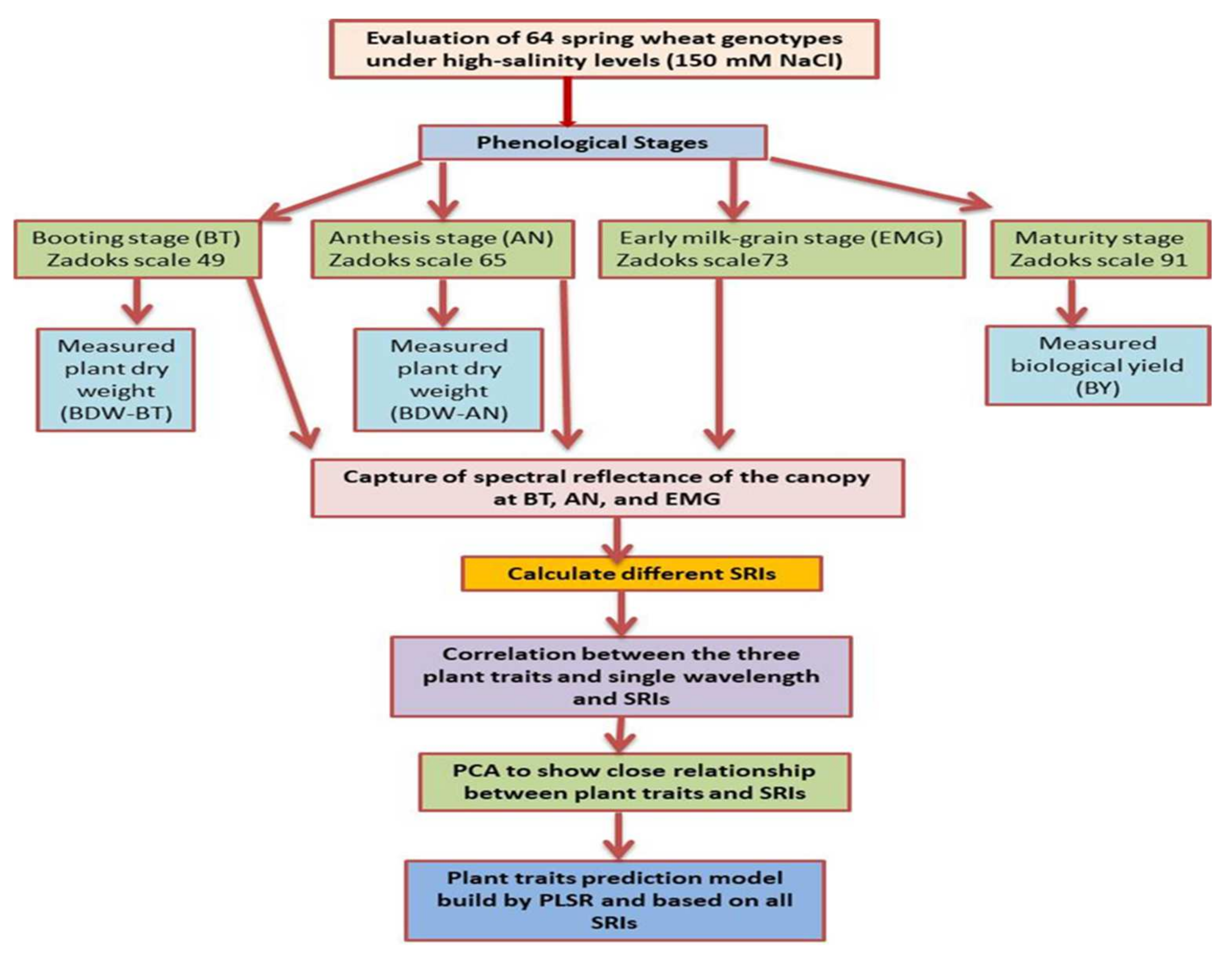
2. Materials and Methods

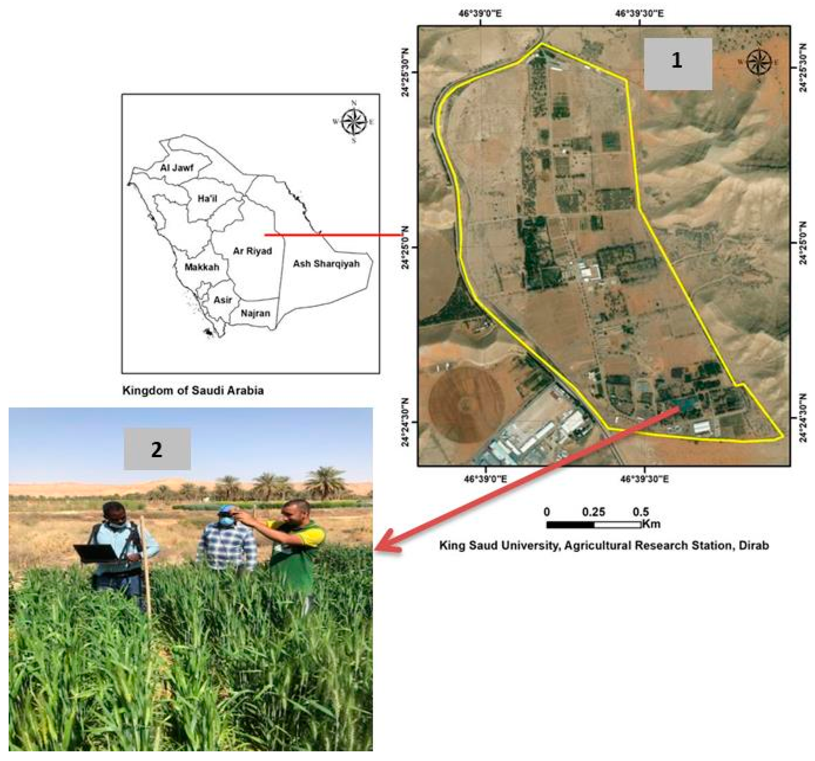
2.1. Plant Materials

The field experiment was conducted in a randomized complete block design with three replications. To generate a wide range of genetic variability in salt tolerance, the experiment included 56 recombinant inbred lines (RILs) of spring wheat, which were developed from the following genetic crosses: between the salt-tolerant genotype Sakha 93 and moderately salt-tolerant genotype Sids 1 (28 RILs), between Sakha 93 and the salt-sensitive genotype Sakha 61 (28 RILs), in addition to five commercial cultivars (Kharchia 65, Misr-1, Shandawel-1, Gemiza-9, and Kawz). These commercial cultivars demonstrated differences in their salt tolerance based on their previous evaluations for salinity tolerance at different growth stages using various agronomic and physiological traits [57,58,59]. All plant material was evaluated under high-salinity levels (150 mM NaCl) during two growing seasons, from 2019 to 2020 and from 2020 to 2021, at the Dierab Research Station of King Saud University in the middle of Saudi Arabia (24°25′ N, 46°34′ E; elevation, 400 m) (Figure 1). At the research station and during the wheat growing season, which is about 150 days, the mean temperature and rainfall ranged from 12.9 °C to 32.2 °C and from 4.0 to 20.0 mm, respectively. Soil texture was sandy loam with electrical conductivity of 1.12 dS m⁻¹, pH of 7.85, organic matter of 0.46%, bulk density of 1.48 g cm⁻³, field capacity of 0.101 m³ m⁻³, and water-holding capacity of 0.066 m³ m⁻³ [60].

The seeds of each genotype were sown on 25 November 2019, and 17 November 2020 in five 1.5 m-long rows spaced 0.2 m apart (1.5 m² in the total area) and at a seeding rate of 15 g m⁻². All genotypes were fertilized with a nitrogen–potassium–phosphorus (NPK) fertilizer at a rate of 150, 120, and 100 kg ha⁻¹, respectively. The entire amount of phosphorus (as calcium superphosphate, 18.5% P₂O₅) and 50 kg ha⁻¹ of each nitrogen (as ammonium nitrate, 33.5 N) and potassium (as potassium chloride, 50% K₂O) were applied before sowing. The plants were fertilized again with 50 kg ha⁻¹ of nitrogen at the late tillering growth stage (Zadoks scale, ZS 28) and with 50 kg ha⁻¹ of nitrogen and potassium at the late booting growth stage (Zadoks scale, ZS 47). The phenology growth stages were defined based on the scale created by Zadoks et al. [61]. Weeds were removed manually, whereas pests and diseases were chemically treated when necessary.

Each genotype was irrigated with fresh water for the first three weeks after sowing to avoid the negative impacts of salinity on germination and seedling establishment. Thereafter, the genotypes were irrigated with artificial saline water containing 150 mM NaCl L⁻¹ solution. The genotypes were irrigated with saline water using a low-pressure surface irrigation system. To deliver saline water from plastic water tanks (5.0 m³) to each plot, the irrigation system consisted of a main line (76 mm in diameter) that branched off to the sub-main hoses at each plot and that was equipped with a manual control valve. Irrigation (frequency and rate) was adjusted according to environmental conditions and plant phenology. On the basis of this information, the genotypes were irrigated with saline water 10 times during their growth stages, with the amount of water totaling 4800 m³ ha⁻¹.

2.2. Measurements of Biomass and Biological Yield

At the booting (BT, ZS 49) and anthesis (AN, ZS 65) growth stages, at about 75 and 90 days from sowing, respectively, 10 plants were randomly selected from the second row of each plot to determine the biomass dry weight (BDW) per plant at BT(BDW-BT) and AN (BDW-AN) stages. The leaves, stems, and spikes of 10 plants were separated, and each part was dried at 70 °C for three days and then weighed to obtain the BDW.

At maturity (on 21 April 2020, and 21 April 2021), the plants from the 1 m-long central two rows of each plot were harvested by hand, air-dried for one week, and weighed to obtain the total biological yield (BY, ton ha⁻¹).

2.3. Spectroradiometric Data and Processing

The spectral reflectance of the canopy for each genotype was captured at the BT, AN, and early milk grain (EMG, ZS 73) growth stages using a FieldSpec 4.0 spectroradiometer (Analytical Spectral Devices (ASD), Malvern Panalytical, Malvern, Worcs, UK), which can detect reflected light from the canopy in the range between 350 and 2500 nm with a final spectral interval of 1 nm and spectral resolution ranging between 3 nm below 1000 nm and 10 nm between 1000 and 2500 nm. The spectral reflectance of the canopy was captured between 11:00 and 15:00 h under clear-sky conditions from two different places within each plot. The optical sensor of the device, which had a field of view of 25°, was placed vertically approximately 1.0 m above the canopy to cover an area of approximately 0.15 m² (approximately 44 cm in diameter). The final reflectance curve for each plot was the average of the spectral reflectance of the two different places with 10 scans for each. A white polytetrafluoroethylene (PTFE) barium sulfate panel (BaSO₄, Spectralon, Labsphere, ASD), which provides a reflectance value of 95–99% over a full spectrum range (350–2500 nm), was used to calibrate the spectral reflectance measurements and to account for any changes in sun irradiance and atmospheric conditions. These calibrations were made on each of the two plots. The spectral reflectance regions between 1830–1940 and 2445–2500 nm were removed from the final reflectance curve and analysis because of high noise levels. The spectral reflectance data in the full-spectrum range (350–2500 nm) were used to test the relationship between spectral reflectance at a single wavelength in the full-spectrum range and target traits. These spectral reflectance data were also used to calculate 13 published and modified SRIs. According to El-Hendawy et al. [19], the modified SRIs were constructed in this study by replacing one or two wavelengths from published SRIs with new wavelengths, but these new wavelengths were still close to those of the published SRIs. The names of these SRIs and their abbreviations and equations are listed in

Table 1. The full name, abbreviation, and equation of published (P) and modified (M) spectral reflectance indices (SRIs) used in this study.

Name and Abbreviation of SRIs	Equation	References
Vegetation-SRIs
Blue normalized difference vegetation index (BNDVI-P)	(R1245 − R415)/(R1245 + R415)	[62]
Blue normalized difference vegetation index (BNDVI-M)	(R1640 − R415)/(R1640 + R415)	This study
Green normalized difference vegetation index (GNDVI-P)	(R1245 − R550)/(R1245 + R550)	[62]
Green normalized difference vegetation index (GNDVI-M)	(R1640 − R550)/(R1640 + R550)	This study
Red normalized difference vegetation index (RNDVI-P)	(R1245 − R680)/(R1245 + R680)	[62]
Red normalized difference vegetation index (RNDVI-M)	(R1640 − R680)/(R1640 + R680)	This study
Red-edge normalized difference vegetation index (RENDVI-P)	(R1100 − R715)/(R1100 + R715)	[62]
Water-SRIs
Water index (WI-M)	(R860/R1640)	This study
Normalized water index -1 (NWI-1-P)	(R970 − R850)/(R970 + R850)	[63]
Normalized difference water index (NDWI-P)	(R860 − R1640)/(R860 + R1640)	[64]
Normalized difference moisture index (NDMI-P)	(R2200 − R1100)/(R2200 + R1100)	[65]
Normalized difference moisture index (NDWI-M1)	(R669 − R1300)/(R669 + R1300)	This study
Normalized difference water index (NDWI-M2)	(R737 − R1360)/(R737 + R1360)	This study

. To make the data processing easier to understand, Figure 2 shows a general flowchart of the methodology proposed for indirectly estimating the plant biomass at different phenological stages.

2.4. Data Analysis

The traits and SRI data were analyzed according to a randomized complete block design using the Proc Mixed procedure in SAS software (v9.4, SAS Institute, Inc., Cary, NC, USA). Data were analyzed in each growing year and growth stage, and in combined years and growth stages. Mean squares of combined analyses were obtained using the Proc Mixed procedure following the TYPE1 method. Pearson’s correlation coefficients (r) were used to test the relationships of plant traits with individual wavelengths in the full-spectrum range and different SRIs at each growth stage and across different growth stages. Principal component analysis (PCA) was conducted to detect the interrelationships between plant traits and all SRIs at each growth stage and across all stages using data from all genotypes over two years. PLSR combined with leave-one-out cross-validation was applied to relate plant traits with all SRIs. The prediction accuracy of the PLSR was evaluated by selecting the optimal number of latent factors (ONLVs). The best ONLVs were those yielding the smallest root mean squared error (RMSE) and largest coefficient of determination (R²). Correlation, PCA, and PLSR analyses were conducted using the XLSTAT statistical package (v2020.1, Excel Add-ins soft, SARL, New York, NY, USA).

3. Results

3.1. Genotypic Variations for Biomass and Biological Yield

Figure S1 displays summary statistical information (the mean, minimum, maximum, analysis of variance (ANOVA), and frequency distribution) of BDW measured at BT (BDW-BT) and AN (BDW-AN) growth stage and BY of 64 wheat genotypes irrigated with a saline water contain 150 mM NaCl. As shown in Supplementary Figure S1, the values of BDW-BT, BDW-AN, and BY across all genotypes ranged between 2.49 and 5.48 g plant⁻¹, 3.49 and 6.83 g plant⁻¹, and 8.90 and 15.41 ton ha⁻¹ in the first year, with average values of 4.19 g plant⁻¹, 5.27 g plant⁻¹, and 12.58 ton ha⁻¹, respectively. In the second year, the BDW-BT, BDW-AN, and BY values ranged between 2.40 and 5.30 g plant⁻¹, 3.93 and 7.76 g plant⁻¹, and 9.13 and 17.88 ton ha⁻¹, with average values of 4.15 g plant⁻¹, 5.41 g plant⁻¹, and 13.81 ton ha⁻¹, respectively. Additionally, the histogram of frequency distribution showed that the three traits were normally distributed in both years. Furthermore, mean squares from the combined ANOVA revealed highly significant differences (p < 0.0001) among genotypes for the three traits, whereas the difference between the years was significant (p < 0.05) for BY only. The interaction effect between genotype and year was significant (p < 0.05) and highly significant (p < 0.0001) for BDW-BT and BDW-AN, respectively (Figure S1).

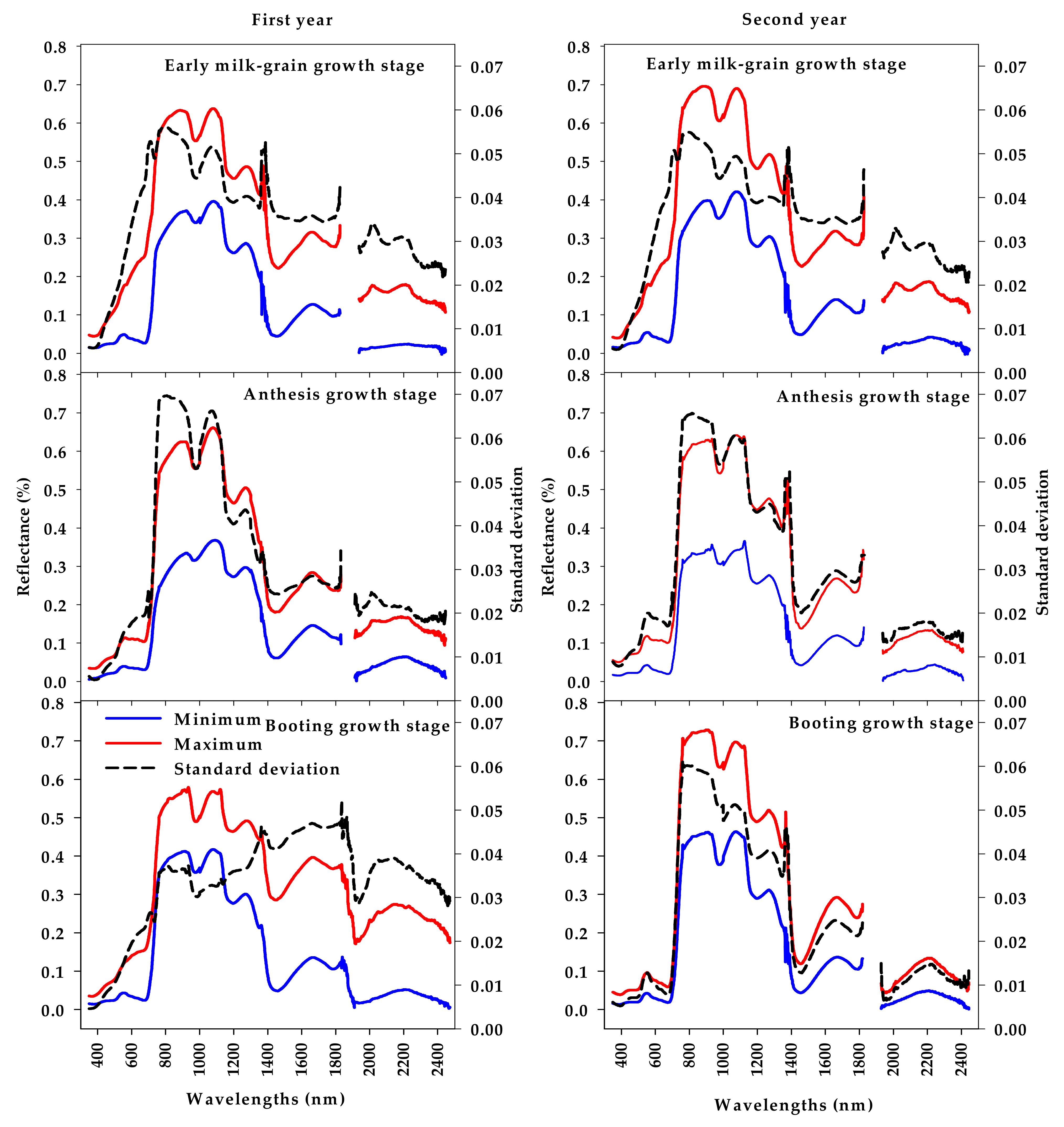
3.2. Analysis of Canopy Spectral Reflectance across Genotypes and Relationship with Biomass and Biological Yield at Different Growth Stages

Figure 3 displays the minimum, maximum, and standard deviations of canopy spectral reflectance in the full range of the spectrum (350–2500 nm) across all genotypes at BT, AN, and EMG stages. Overall, the shape of the spectral reflectance curves in Figure 3 shows that there are obvious differences between the minimum and maximum values of spectral reflectance across all genotypes at the three main regions of the spectrum (VIS, NIR, and SWIR) at each growth stage. In the VIS region, the differences between the minimum and maximum values of the spectral reflectance curve were large at the EMG stage. Compared to the other two stages, the green peak (approximately 550 nm) at the EMG stage was expanded and distorted for the curve of the maximum values (Figure 3). The differences between the minimum and maximum values of the spectral reflectance curve in the NIR region were large at the three stages, except at the BT stage in the first year. The differences between the minimum and maximum values of the spectral reflectance curve in the SWIR region showed very similar patterns at the three stages, except the BT stage in the first year, which indicated obvious differences between the minimum and maximum values in this region (Figure 3).

The results in Figure 3 also revealed that the spectral reflectance at the EMG stage presented higher standard deviations in the VIS and SWIR regions, compared to the other two stages, except the BT stage in the first year, which also presented a high value of standard deviations in the SWIR region. However, the high value for standard deviations of spectral reflectance in the NIR region was observed at the AN stage, as compared with the other two stages (Figure 3).

The Pearson’s correlation coefficient (r) between spectral reflectance at a single wavelength in the three regions of the spectrum and the three traits at the three growth stages are shown in Figure 4. In general, the results showed that the wavelengths in the VIS region were negatively correlated with the three traits at the three growth stages in both years, whereas the whole wavelength in the NIR region was positively correlated with the same traits at the AN and EMG stages. At the BT stage, the red-edge region (700–750 nm) and wavelengths between 1150–1300 nm in the NIR region exhibited a negative correlation with the three traits, and a positive correlation was expressed in the wavelength region between 750–1150 nm (Figure 4). The signs of r between the SWIR wavelengths and three traits depended on the growth stage: r was negative at the BT and AN stages, whereas it was positive at the EMG stage (Figure 4). Additionally, the wavelengths in the three regions of the spectrum showed a higher correlation with the BDW-AN trait than those of the BDW-BT and BY traits at the BT and AN stages, and they were best correlated with the BY trait, followed by the BDW-AN trait, at the EMG stage (Figure 4). The wavelengths in the VIS region showed no significant correlation with any trait at the BT stage, and they showed weak to strongly significant correlations (r ranged from −0.25 to −0.80) with all traits at the AN and EMG stages. The wavelengths in the NIR region had a weak to strong positive correlation (r ranged from 0.25 to 0.82) with the three traits at the AN and EMG stages, and the red-edge band was the only wavelength range in the NIR region that exhibited a weak to strong negative correlations (r ranged from −0.30 to −0.75) with the three traits at the BT stage (Figure 4). At the BT stage, the wavelengths in the SWIR region exhibit a weak to strong correlation (r ranged from −0.30 to −0.75) with the three traits in both years, and the correlation depended on the traits and year in the AN and EMG stages. In the first year, most wavelengths in the SWIR region were only moderately correlated with the BDW-AN trait at the AN stage and the BY trait at the EMG stage. In the second year, these wavelengths exhibited a moderate correlation with only the BDW-AN trait at the AN stage and three traits at the EMG stage (Figure 4).

3.3. Genotypic Variations for Spectral Reflectance Indices and Their Relationship with Biomass and Biological Yield

Table 2. Mean squares and degrees of freedom (df)for the effects of year (Y), growth stage (GS), genotypes (G), and their possible interaction by ANOVA on different spectral reflectance indices (SRIs).

Effect	Y	GS	GS × Y	G	G × Y	G × GS	G × GS × Y
dF	1	2	2	63	63	126	126
Vegetation-SRIs
BNDVI-P	0.0114 **	0.0817 ***	0.0731 ***	0.0120 ***	0.0032 ***	0.0066 ***	0.0034 ***
BNDVI-M	0.1969 **	0.0366 ***	0.2666 ***	0.0160 ***	0.0103 ***	0.0202 ***	0.0104 ***
GNDVI-P	0.0011 ns	1.9338 ***	0.0500 ***	0.0578 ***	0.0120 ***	0.0305 ***	0.0123 ***
GNDVI-M	0.2608 **	2.0079 ***	0.1929 ***	0.0530 ***	0.0294 ***	0.0596 ***	0.0293 ***
RNDVI-P	0.8169 **	5.6678 ***	0.2006 ***	0.0922 ***	0.0148 ***	0.0524 ***	0.0164 ***
RNDVI-M	1.1368 *	8.8531 ***	0.3262 ***	0.1073 ***	0.0365 ***	0.1005 ***	0.0348 ***
RENDVI-P	0.1400 **	4.6975 ***	0.0295 **	0.0130 ***	0.0102 ***	0.0143 ***	0.0097 ***
Water-SRIs
WI-M	68.3056 **	34.2353 ***	16.7869 ***	1.8441 ***	0.3190 ***	0.7575 ***	0.6815 ***
NWI-1-P	0.1229 **	0.0291 ***	0.0390 ***	0.0016 ***	0.0007 ***	0.0007 ***	0.0008 ***
NDWI-P	1.3212 ***	0.6691 ***	0.3359 ***	0.0471 ***	0.0103 ***	0.0183 ***	0.0172 ***
NDMI-P	0.9310 **	0.3763 ***	0.2314 ***	0.0295 ***	0.0119 ***	0.0143 ***	0.0141 ***
NDWI-M1	0.7614 **	5.4684 ***	0.1913 ***	0.0896 ***	0.0149 ***	0.0516 ***	0.0161 ***
NDWI-M2	0.7219 **	0.1230 ***	0.4228 ***	0.0354 ***	0.0072 ***	0.0194 ***	0.0133 ***

*, **, ***: indicate significance at p ≤ 0.05, 0.01, and 0.001, respectively, and ns indicate not significant. The full names of the abbreviations SRIs are listed in Table 1.

and

Table 3. Statistical parameters (minimum (Min), maximum (Max), mean values, mean standard error (MSE), and LSD) for different spectral reflectance indices (SRIs) at each growth stage and combined all stages across 64 wheat genotypes grown in 150 mM NaCl.

SRIs	Booting Stage					Anthesis Stage
	Min	Max	Mean	MSE	LSD	Min	Max	Mean	MSE	LSD
BNDVI-P	0.768	0.917	0.864	0.003	0.047 ***	0.720	0.931	0.857	0.005	0.026 ***
BNDVI-M	0.551	0.838	0.740	0.007	0.092 ***	0.601	0.832	0.740	0.005	0.059 ***
GNDVI-P	0.547	0.810	0.705	0.006	0.084 ***	0.458	0.828	0.676	0.010	0.047 ***
GNDVI-M	0.219	0.651	0.478	0.011	0.140 ***	0.257	0.609	0.456	0.008	0.089 ***
RNDVI-P	0.584	0.891	0.806	0.007	0.077 ***	0.551	0.890	0.745	0.011	0.051 ***
RNDVI-M	0.254	0.797	0.641	0.012	0.130 ***	0.315	0.730	0.563	0.011	0.085 ***
RENDVI-P	0.453	0.662	0.587	0.006	0.056 ***	0.474	0.639	0.555	0.005	0.040 ***
WI-M	1.626	3.515	2.812	0.049	0.542 ***	1.480	3.940	2.644	0.070	0.590 ***
NWI-1-P	−0.086	−0.022	−0.063	0.002	0.015 ***	−0.075	−0.007	−0.056	0.002	0.012 ***
NDWI-P	0.238	0.557	0.466	0.008	0.078 ***	0.193	0.595	0.436	0.011	0.071 ***
NDMI-P	−0.799	−0.487	−0.712	0.007	0.074 ***	−0.809	−0.531	−0.696	0.008	0.058 ***
NDWI-M1	−0.890	−0.580	−0.803	0.007	0.078 ***	−0.890	−0.553	−0.744	0.011	0.051 ***
NDWI-M2	−0.080	0.117	0.030	0.004	0.060 ***	−0.233	0.234	0.053	0.012	0.098 ***
	Early milk-grain stage					Across three stages
	Min	Max	Mean	MSE	LSD	Min	Max	Mean	MSE	LSD
BNDVI-P	0.701	0.919	0.834	0.005	0.025 ***	0.792	0.904	0.853	0.003	0.020 ***
BNDVI-M	0.496	0.853	0.721	0.009	0.043 ***	0.649	0.807	0.736	0.004	0.039 ***
GNDVI-P	0.266	0.773	0.569	0.013	0.056 ***	0.512	0.768	0.649	0.007	0.037 ***
GNDVI-M	−0.051	0.623	0.343	0.016	0.077 ***	0.257	0.568	0.422	0.007	0.061 ***
RNDVI-P	0.196	0.837	0.570	0.019	0.070 ***	0.480	0.852	0.700	0.009	0.038 ***
RNDVI-M	−0.079	0.737	0.351	0.024	0.091 ***	0.289	0.712	0.499	0.011	0.060 ***
RENDVI-P	0.275	0.527	0.379	0.007	0.036 ***	0.423	0.568	0.500	0.003	0.026 ***
WI-M	1.551	2.969	2.252	0.032	0.222 ***	1.798	3.142	2.521	0.037	0.276 ***
NWI-1-P	−0.077	−0.001	−0.044	0.001	0.010 ***	−0.074	−0.028	−0.055	0.001	0.007 ***
NDWI-P	0.216	0.496	0.381	0.006	0.043 ***	0.285	0.517	0.427	0.006	0.038 ***
NDMI-P	−0.766	−0.511	−0.650	0.006	0.510 ***	−0.761	−0.551	−0.685	0.005	0.036 ***
NDWI-M1	−0.838	−0.205	−0.572	0.019	0.069 ***	−0.851	−0.482	−0.700	0.009	0.038 ***
NDWI-M2	−0.050	0.176	0.061	0.005	0.040 ***	−0.064	0.136	0.048	0.005	0.041 ***

***: indicate significance at p ≤ 0.001. The full names of the abbreviations SRIs are listed in Table 1.

display summary statistical information (ANOVA analysis, minimum, maximum, mean, LSD, and significant level of F-test) for different vegetation- and water-related SRIs calculated at different growth stages. Mean squares from the ANOVA analysis combined over years and growth stages revealed that year, growth stage, and genotype main effects were highly significant (p < 0.001 and 0.0001) for all SRIs, except the published green normalized difference vegetation index (GNDVI-P), for which the year effect was not significant. The two-way (growth stage × year, genotype × year, and genotype × growth stage) and three-way (genotype × growth stage × year) interactions were highly significant for all SRIs (Table 2).

The results in Table 3 also revealed a wide range between the minimum and maximum values among genotypes for all SRIs at the three stages. For nearly all SRIs, the maximum values were two to four times higher than the minimum values. Additionally, the values of all vegetation-related SRIs and two indices from water-related SRIs (the modified water index (WI-M) and published normalized difference water index (NDWI-P) showed a continuous decrease from the BT to the EMG stage. By contrast, the values of other water-related SRIs increased from the BT to the EMG stage (Table 3).

The relationships between SRIs and the three traits at each growth stage, across three growth stages for each year, and across two years are presented in

Table 4. Correlation coefficients for the relationships between different vegetative- and water-SRIs and plant dry weight measured at booting (BDW-BT) and anthesis (BDW-AN) growth stage and biological yield (BY) across 64 wheat genotypes grown in 150 mM NaCl at each growth stage and across three stages for each year and across two years (com.).

SRIs	Booting Stage									Across Stages
	BDW-BT			BDW-AN			BY
	1st Year	2nd Year	Com.	1st Year	2nd Year	Com.	1st Year	2nd Year	Com.	BDW-BT
BNDVI-P	−0.04	−0.14	−0.09	−0.19	−0.07	−0.14	−0.13	−0.03	−0.14	0.61
BNDVI-M	−0.24	−0.23	−0.29	−0.43	−0.16	−0.39	−0.31	−0.13	−0.35	0.44
GNDVI-P	−0.03	−0.13	−0.10	−0.16	−0.09	−0.14	−0.10	−0.06	−0.14	0.61
GNDVI-M	−0.24	−0.22	−0.31	−0.40	−0.18	−0.40	−0.30	−0.15	−0.36	0.48
RNDVI-P	0.02	−0.11	−0.03	−0.11	−0.09	−0.11	−0.06	−0.02	−0.08	0.65
RNDVI-M	−0.11	−0.18	−0.18	−0.26	−0.17	−0.30	−0.17	−0.10	−0.24	0.60
RENDVI-P	0.60	0.62	0.71	0.77	0.75	0.88	0.65	0.60	0.71	0.39
WI-M	0.63	0.46	0.65	0.77	0.51	0.82	0.57	0.52	0.68	0.60
NWI-1-P	−0.64	−0.45	−0.64	−0.74	−0.53	−0.79	−0.56	−0.51	−0.66	−0.57
NDWI-P	0.61	0.42	0.62	0.75	0.48	0.80	0.57	0.52	0.68	0.60
NDMI-P	−0.63	−0.47	−0.66	−0.75	−0.66	−0.83	−0.60	−0.54	−0.68	−0.52
NDWI-M1	−0.01	0.12	0.04	0.12	0.10	0.13	0.07	0.03	0.09	−0.65
NDWI-M2	0.49	−0.02	0.35	0.62	0.03	0.48	0.46	0.03	0.43	0.55
	Anthesis Stage									BDW-AN
BNDVI-P	0.63	0.43	0.65	0.74	0.69	0.83	0.50	0.45	0.54	0.77
BNDVI-M	0.52	0.26	0.55	0.46	0.48	0.58	0.30	0.30	0.38	0.52
GNDVI-P	0.67	0.46	0.67	0.83	0.71	0.88	0.53	0.46	0.55	0.80
GNDVI-M	0.60	0.35	0.65	0.62	0.58	0.75	0.35	0.36	0.45	0.60
RNDVI-P	0.61	0.46	0.65	0.80	0.72	0.88	0.50	0.42	0.55	0.82
RNDVI-M	0.57	0.41	0.64	0.65	0.69	0.80	0.38	0.35	0.46	0.74
RENDVI-P	0.27	0.06	0.12	0.45	0.36	0.34	0.08	0.13	0.19	0.53
WI-M	0.46	0.40	0.51	0.76	0.73	0.84	0.39	0.39	0.47	0.88
NWI-1-P	−0.45	−0.13	−0.34	−0.66	−0.43	−0.60	−0.23	−0.15	−0.29	−0.78
NDWI-P	0.47	0.41	0.51	0.78	0.70	0.83	0.41	0.41	0.49	0.86
NDMI-P	−0.40	−0.30	−0.40	−0.66	−0.53	−0.68	−0.32	−0.22	−0.34	−0.76
NDWI-M1	−0.62	−0.46	−0.65	−0.79	−0.72	−0.88	−0.51	−0.42	−0.55	−0.81
NDWI-M2	0.42	0.38	0.50	0.68	0.62	0.76	0.34	0.39	0.42	0.80
	Early Milk-Grain Stage									BY
BNDVI-P	0.36	0.54	0.54	0.54	0.66	0.70	0.61	0.71	0.74	0.65
BNDVI-M	0.26	0.51	0.48	0.43	0.63	0.64	0.54	0.68	0.72	0.52
GNDVI-P	0.34	0.53	0.52	0.53	0.62	0.68	0.63	0.69	0.72	0.66
GNDVI-M	0.24	0.51	0.47	0.43	0.61	0.64	0.56	0.67	0.71	0.56
RNDVI-P	0.41	0.56	0.57	0.56	0.67	0.71	0.65	0.73	0.73	0.71
RNDVI-M	0.34	0.56	0.54	0.51	0.68	0.69	0.63	0.73	0.74	0.68
RENDVI-P	0.09	−0.24	−0.09	−0.04	−0.23	−0.16	−0.17	−0.30	−0.31	0.26
WI-M	0.19	−0.10	0.12	0.23	−0.13	0.16	0.08	−0.08	0.02	0.55
NWI-1-P	−0.20	0.04	−0.23	−0.22	0.06	−0.25	−0.26	−0.06	−0.23	−0.55
NDWI-P	0.23	−0.08	0.18	0.25	−0.10	0.20	0.14	−0.03	0.08	0.58
NDMI-P	−0.10	0.14	−0.02	−0.12	0.14	−0.07	−0.09	0.09	−0.02	−0.50
NDWI-M1	−0.41	−0.56	−0.57	−0.56	−0.67	−0.71	−0.65	−0.73	−0.74	−0.71
NDWI-M2	0.19	0.06	0.31	0.31	0.07	0.38	0.36	0.21	0.38	0.53

Bold values indicate significant at 0.05, 0.01, 0.001 probability level. The full name of the abbreviation SRIs is listed in Table 1.

.

In general, nearly all SRIs exhibited strong correlations with BDW-BT (r > 0.64 or <−0.64), BDW-AN (r > 0.85 or <−0.81), and BY (r > 0.70 or <−0.70) when data from two years and different growth stages were combined. In most cases, the correlation coefficients between SRIs and the three traits for an individual year were lower than the coefficients using two-year combinations (Table 4). All water-related SRIs, except the modified normalized difference water index-1 (NDWI-M1) and one index from vegetation-related SRIs (i.e., the published red-edge normalized difference vegetation index (RENDVI-P)), provided a moderate to strong correlation with the three traits at the BT stage. The opposite was true at the EMG stage, whereas nearly all vegetation- and water-related SRIs exhibited moderate to strong correlations with the three traits at the AN stage (Table 4).

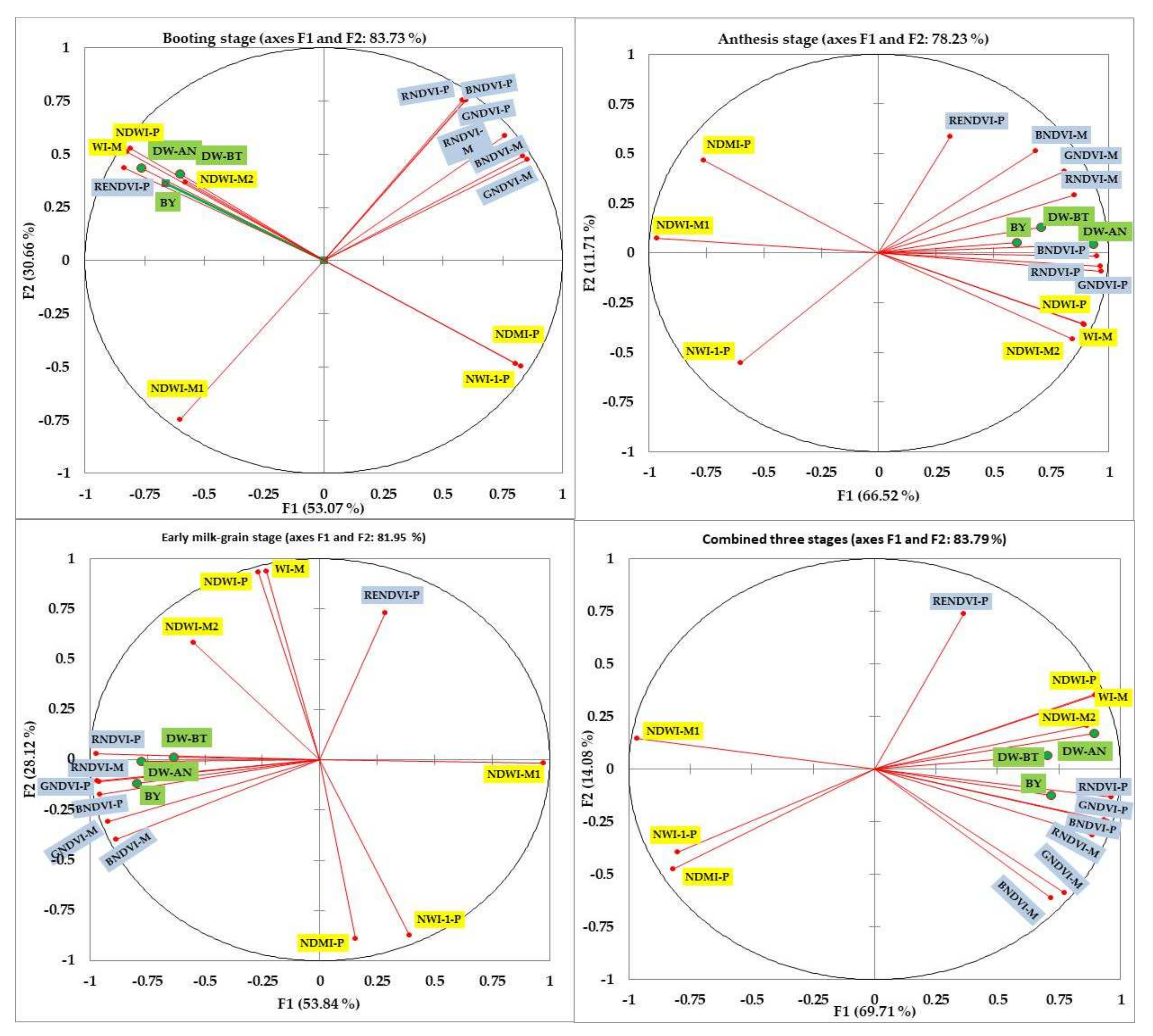
3.4. Principal Component Analysis

PCA was conducted to compare all SRIs and to show which SRIs are close to plant traits. The results from PCA showed that the first factor (PC1) explained 53.1%, 66.5%, 53.8%, and 69.7% of the total variation whereas the second factor (PC2) explained 30.7%, 11.7%, 28.1%, and 14.1% of the total variation at the BT, AN, EMG, and combined three growth stages, respectively (Figure 5). At the BT stage, the three measured traits were grouped together with three water-related SRIs (WI-M, NDWI-P, and NDWI-M2) and one published vegetation-related SRI (RENDVI-P) in a negative PC1 slope, with an acute angle between the vectors of three traits and these four SRIs. The three traits were grouped with the same three water-related SRIs (WI-M, NDWI-P, and NDWI-M2) and all vegetation-related SRIs with a positive PC1 slope at the AN stage and in the combined three stages, and in a negative PC1 slope (except RENDVI-P) at the EMG stage, with an acute angle between the vectors of three traits and these SRIs (Figure 5). At each growth stage and in the combined three stages, the angle between the vectors of the three traits and other water-related SRIs was obtuse and straight (Figure 5). In general, an acute angle indicates a strong positive association between SRIs and the three traits. The opposite is indicated with obtuse and straight angles.

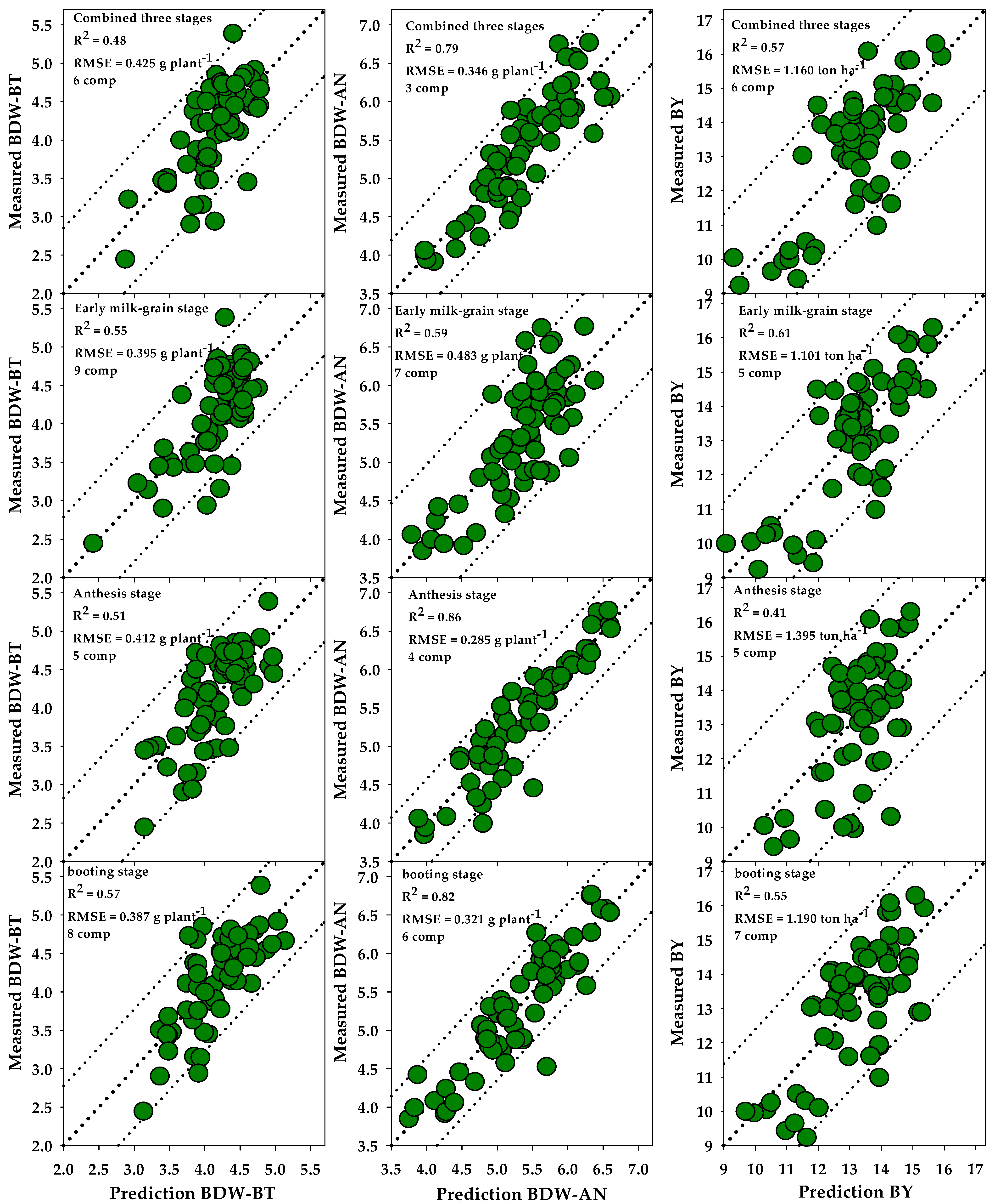
3.5. Prediction of Biomass and Biological Yield Based on All SRIs Using PLSR Models

Figure 6 shows the relationship between the measured and predicted values of the BDW-BT, BDW-AN, and BY traits at each growth stage and in the combined three stages by the PLSR models and based on all SRIs. The optimum number of components was estimated via cross-validation and selected on the basis of the best PLSR model that gave high and low values for R² and RMSE, respectively. The optimum number ranged from five to nine for the BDW-BT trait, from three to seven for the BDW-AN trait, and from five to seven for BY when the data were analyzed for each growth stage separately or for the combined three stages together (Figure 6). For the BDW-BT trait, predictive ability was good at the BT (R² = 0.57) and EGM (R² = 0.55) stages and moderate at the AN stage (R² = 0.51) and combined three stages (R² = 0.48). For the BDW-AN trait, predictive ability was strongest at the BT, AN, and combined three stages (R² = 0.79–0.86) and good at the EGM stage (R² = 0.59). For BY, predictive ability was strongest at the EMG stage (R² = 0.61), good at the BT stage (R² = 0.55) and combined three growth stages (R² = 0.57), and moderate at the AN stage (R² = 0.41) (Figure 6).

4. Discussion

Previous studies have reported that whole-plant biomass is considered one of the most useful phenotypic traits to evaluate genotypes in breeding programs under both normal and stress conditions. This is because this plant trait reflects several physiological processes, integrates plant responses to stresses at the whole-plant level and at different growth stages, and is directly related to radiation use efficiency and final crop production [19,21,22,28,66,67]. Interestingly, this study confirmed that plant biomass measured at booting (BDW-BT) and anthesis (BDW-AN) growth stages, as well as the BY measured at maturity, are important phenotypic traits for differentiating salt tolerance among genotypes. We observed a sufficient genotypic variation for these traits (i.e., genotype had a highly significant main effect on these traits (p < 0.0001) with a wide range between the minimum and maximum values for these traits across genotypes (Figure S1). This wide range of genotypic variation in plant biomass at different growth stages indicates that some tested genotypes might possess more efficient mechanisms than others to cope with the osmotic injury and specific ion toxicity effects of salinity stress. This further indicates that measurements of biomass at different growth stages can be used as potential screening criteria for differentiating salt tolerance behavior between wheat genotypes. Unfortunately, the direct assessment of plant biomass based on destructive sampling methods is generally time- and cost-inefficient, tedious, and unable to detect the dynamic changes of this trait in real time. Tools that are rapid, nondestructive, and cost-efficient are therefore urgently needed to assess plant biomass, particularly when plant breeders wish to incorporate this plant trait into breeding programs as screening criteria to evaluate the salt tolerance of a large number of genotypes across different growth stages.

In general, exposing plants to high-salinity levels leads to noticeable changes and modifications in several morphological, anatomical, biochemical, and physiological plant characteristics [5,68,69,70]. Fortunately, the characteristics of spectral signatures that are reflected from the plant canopy at specific full-spectrum wavelengths using hyperspectral sensors are usually closely associated with these changes [5,42,45,71,72]. This reveals that it is possible to rapidly and nondestructively assess plant biomass for large germplasm collections based on genotypic variation in the spectral reflectance behavior over the full-spectrum range. Interestingly, the results in Figure 1 revealed that there are obvious differences between the minimum and maximum values of spectral reflectance across all genotypes in the three main regions of the spectrum at three different growth stages, with a few exceptions. Additionally, the standard deviation of spectral reflectance across all genotypes is highest in the VIS and SWIR regions at the EMG stage and in the three regions of the spectrum at the AN stage (Figure 3). This genotypic variation in spectral reflectance behavior makes the hyperspectral reflectance tool a promising technique for providing crucial information for genotype selection and management of abiotic stresses and allows for the effective evaluation of a large number of genotypes without compromising the accuracy of conventional phenotyping methods through repetitive assessments of screening criteria of interest. The results in Figure 4 further confirmed this and indicated that the three traits (BDW-BT, BDW-AN, and BY) showed significant correlation with the wavelengths in the three regions of the spectrum. However, the value of correlation between traits and wavelengths depends on growth stages. The wavelengths in the VIS region exhibited a weak correlation (not significant) with the three traits at the BT stage, and they showed weak to strong correlations (r ranged from −0.25 to −0.80) with the three traits at the AN and EGM stages. The three traits were better correlated with wavelengths in the SWIR region than with wavelengths in the NIR region at the BT stage, and the opposite was found at the AN and EMG stages, with a few exceptions (Figure 4). These findings revealed that in using hyperspectral reflectance tools, specific wheat growth stages must be taken into account when phenotyping the plant traits for a large number of genotypes. These findings also suggest that the hyperspectral reflectance tool can be applicable in salinity studies for assessing plant biomass and for effectively screening wheat genotypes at the early growth stage, obviating the need to grow genotypes to maturity, but this suggestion is only applicable by looking at specific wavelengths in the red-edge and SWIR regions as shown in Figure 4. Generally, the spectral reflectance at wavelengths in the VIS, NIR, and SWIR regions is affected primarily by the vegetation growth status (contents of chlorophyll and other photosynthetic pigments), plant biomass status (cumulative plant biomass, canopy structure, and leaf cellular structure), and plant water status (content of canopy water and material absorbed light such as lignin, cellulose, protein, and cell walls), respectively [73,74,75,76,77,78]. According to Munns and Tester [24], plant biomass responds to salinity stress in two phases, referred to as the osmotic phase and ionic phase. In the first phase, the plant canopy begins to show symptoms of a water deficit because the high salt concentrations in the root zone restrict the capacity of roots to uptake sufficient water. In the second phase, which corresponds to the build-up of harmful ions (Na⁺ and Cl⁻) in the leaves, necrosis and senescence are the main canopy symptoms. These two phases of salinity stress, in addition to the close relationship between spectral reflectance at specific wavelengths and plant canopy characteristics may explain why the relationships between SWIR wavelengths and plant biomass are stronger at the early stage (BT) than those in the VIS and NIR regions, and vice versa at the later stages (AN and EMG stages).

4.1. Identification of the Best Spectral Reflectance Indices and Growth Stage for Indirect Biomass Assessment

Previous studies have reported that SRIs can be used as indirect alternative evaluation tools for providing rapid and accurate assessment of stress-related traits [13,17,19,50,79,80]. However, SRI type (vegetation- or water-based), sampling date (phenological growth stages), and the degree of genotypic variation for SRIs play a key role in the capability of SRIs to accurately assess and monitor plant traits of interest. In the case of the SRI type, previous studies reported that in capturing genotypic variability in grain yield and biomass under diverse environmental conditions, water-related SRIs, which are calculated from wavelengths located in the NIR and SWIR regions, always performed better than the vegetation-related SRIs, which are calculated from wavelengths located in the VIS and red-edge regions [19,36,63,79,81]. Because there is a significant interaction between growth stages and genotypes for different SRIs, the suitable growth stage for assessing the plant traits based on SRIs must be cautiously identified to accurate assessment of the most effective plant traits among genotypes. In wheat, most previous studies reported that the majority of SRIs were sensitive to variation in measured plant traits (i.e., plant biomass and grain yield) when recorded after the heading stage (AN and EMG stages). Combining SRIs across multiple stages also gave a better correlation with plant traits than any individual growth stage [17,21,44,63,79,81,82,83]. This study dealt with the abovementioned three factors and found that a significant genotypic variation was observed for all SRIs (Table 2), with a wide range between the minimum and maximum values for these indices at different stages separately and across three stages (Table 3). This finding indicates that effective genetic gain in plant biomass under salinity stress could be obtained by evaluating genotypes based on SRIs and that these SRIs could be used as alternative selection criteria for fast and accurate assessments of salinity tolerance in a spring wheat-breeding program. However, we observed the interaction of growth stages with genotypes for different SRIs in this study (Table 2). This emphasizes that the appropriate growth stage for assessing plant biomass under salinity conditions using SRIs must be precisely identified for the accurate assessment of the salt tolerance of wheat genotypes in breeding programs. The results presented in Table 4 confirmed this finding and further revealed that the appropriate growth stage for assessing plant biomass also depends on the type of SRIs. At the BT stage, all water-related SRIs, except NDWI-M1, and only one index from vegetation-related SRIs (RENDVI-P) were found to be efficient for assessing the three traits; the opposite was true at the EMG stage. However, nearly all vegetation- and water-related SRIs were similarly well suited to assess the three traits at the AN stage (Table 4). All of these results implied that the variation in plant biomass among genotypes can be assessed at the early growth stage (BT) using the water-related SRIs, which detect plant water status, and the late growth stage (EMG) is appropriate for vegetation-related SRIs, which reflects the chlorophyll and growth status of plants. The AN stage is the appropriate developmental stage for plant biomass assessment, using a combination of vegetation- and water-related SRIs. These results confirmed the importance of two phases of plant response to salinity stress described by Munns and Tester [24]. Additionally, the visible wavelengths incorporated in the vegetation-related SRIs (especially red light) are usually saturated at a high leaf area index and high concentration of different pigments; this may explain why vegetation-related SRIs failed to assess plant biomass at the BT stage. However, as growth progresses from the BT to EMG stage, these kinds of indices become effective for assessing plant biomass because necrosis and senescence symptoms start to appear on the leaves as a real phenomenon of salinity damage, and genotypic differences in biomass and chlorophyll contents are also high at later stages. This also confirms why the mean values of vegetation-related SRIs decrease from the BT to the EMG stage (Table 3). Furthermore, because multiple measurements of spectral reflectance of genotypes across multiple growth stages capture overall the effects of salinity stress on various physiological attributes that ultimately cumulatively affect plant biomass and yield, this may be the reason that nearly all SRIs successfully assess plant biomass when the SRI data are analyzed together across the three growth stages (Table 4). Therefore, in all cases, our results suggest that it is possible to detect genotypic variation in plant traits related to biomass accumulation under high-salinity stress at early growth stages based on SRIs.

The results of the PCA presented in Figure 5, in which all indices and their relationship with the three plant traits are shown together, fully confirmed the abovementioned findings and showed that the angle of the vectors of the three traits was acute in three cases: (1) with three water-related SRIs (WI-M, NDWI-M2, and NDWI-P) and one vegetation-related SRI (RENDVI-P) at the BT stage; (2) with all vegetation-related SRIs, except RENDVI-P, at the EMG stage; and (3) with a combination of these former indices at the AN stage and across three stages. However, the angle between the vectors of the remaining indices and the three traits was obtuse or straight at each growth stage or across three stages (Figure 5). Generally, the acute angle between SRIs and traits reflects the ability of these indices to effectively assess genotypic variation in plant biomass. The obtuse and straight angles between SRIs and traits indicate that these indices could be used as a complementary selection tool with other indices to detect genotypic differences in plant biomass. The results of PCA indicate that the water-related SRIs are more effective in assessing plant biomass than vegetation-related SRIs at an early growth stage; the opposite is true at a late growth stage. Additionally, each type of SRI measures related parameters, confirming the importance of the two phases of plant response to salinity stress described by Munns and Tester [24].

4.2. Prediction of Plant Biomass and Biological Yield Based on PLSR

The performance of SRIs for estimating the three plant traits depends on the growth stage and type of SRIs. Additionally, almost all vegetation-related SRIs were grouped in one dimension as shown in PCA (Figure 5). One reason for these findings may be that the different SRIs are always formulated based on two to three sensitive wavelengths, making it difficult to build a unified index that includes enough wavelengths that are sensitive to all biophysical and biochemical changes that logically occur in plants in diverse phenological stages. These limited wavelengths in each index make it difficult to overcome the impacts of growth conditions, soil background, and saturation of the leaf area index, chlorophyll content, and biomass on the performance of the index of interest. The same type of SRIs exhibits high multicollinearity among themselves, which reduces the ability of such indices to detect a variation among genotypes that exhibit similar reflectance and absorption behavior. Therefore, previous studies have reported that using a combination of SRIs and multivariate regression models such as PLSR can overcome these limitations and significantly improve the predication accuracy of relevant plant traits [43,52,54,80,82,84,85,86,87,88,89]. Most of these studies reported that using several SRIs in tandem with the PLSR model resulted in better performance in the estimation of plant traits, such as plant biomass, grain yield, and plant water content, as compared with a single index. In this study, by combining SRIs with PLSR, assessing plant biomass at the early growth stage was possible. Interestingly, by coupling both methods, a good prediction of BDW-BT (57%), BDW-AN (82%), and BY (55%) was obtained at the BT stage (Figure 6). However, the highest predictions of BDW-BT, BDW-AN, and BY were obtained at the BT (57%), AN (86%), and EMG (61%) stages, respectively (Figure 6). The results in Figure 4 generally suggest that the combination of different SRIs and PLSR models is a promising approach to predict the plant biomass of a large number of wheat genotypes under high-salinity conditions at the BT stage because this combination can simultaneously cover several response variables and can account for multicollinear variables.

5. Conclusions

The results of this study showed that the response plant biomass of a large number of wheat genotypes to salinity stress at different growth stages can be assessed using the rapid, nondestructive, and relatively inexpensive hyperspectral reflectance tool. Significant genotypic differences were observed in canopy spectral reflectance at the three regions of the spectrum (VIS, NIR, and SWIR) with a significant correlation between a single wavelength within these regions and the three plant traits related to biomass accumulation. Furthermore, the significant correlation between SRIs confirmed the potential of hyperspectral reflectance data as a simple and easy way to assess plant biomass for a large number of genotypes. However, the growth stage and type of SRIs played a key role in the capability of SRIs to accurately assess and monitor plant biomass. Water-based SRIs were much more effective than vegetation-related SRIs for assessing plant biomass at the BT stage; the opposite was found at the EMG stage. Both types of SRIs demonstrated consistently higher levels of association with plant biomass at the AN stage. Interestingly, by coupling SRIs with the PLSR model, an assessment of the plant biomass at the early stage (BT) was possible. Combining both methods resulted in a good prediction of BDW-BT (57%), BDW-AN (82%), and BY (55%) at the BT stage. Finally, our findings confirmed the importance of hyperspectral reflectance data and multivariate analysis in evaluating the salt tolerance of a large number of genotypes in wheat-breeding programs.

References

1. FAOSTAT. Food and Agriculture Organization of the United Nations Statistics Database, Rome. 2021. Available online: http://www.fao.org/faostat/en/#home (accessed on 15 February 2021).
2. Curtis, B.C. Wheat in the World. Available online: http://www.fao.org/3/y4011e/y4011e04.htm (accessed on 28 March 2019).
3. Grote, U.; Fasse, A.; Nguyen, T.T.; Erenstein, O. Food security and the dynamics of wheat and maize value chains in Africa and Asia. Front. Sustain. Food Syst. 2021, 4, 617009. [Google Scholar] [CrossRef]
4. Rengasamy, P. Soil processes affecting crop production in salt-affected soils. Funct. Plant Biol. 2010, 37, 613–620. [Google Scholar] [CrossRef]
5. El-Hendawy, S.E.; Hassan, W.M.; Al-Suhaibani, N.A.; Refay, Y.; Abdella, K.A. Comparative performance of multivariable agro-physiological parameters for detecting salt tolerance of wheat cultivars under simulated saline field growing conditions. Front. Plant. Sci. 2017, 8, 435. [Google Scholar] [CrossRef] [PubMed] [Green Version]
6. Wang, Z.; Fan, B.; Guo, L. Soil salinization after long-term mulched drip irrigation poses a potential risk to agricultural sustainability. Eur. J. Soil Sci. 2019, 70, 20–24. [Google Scholar] [CrossRef] [Green Version]
7. Sheoran, P.; Kumar, A.; Sharma, R.; Prajapat, K.; Kumar, A.; Barman, A.; Raju, R.; Kumar, S.; Dar, Y.J.; Singh, R.K.; et al. Quantitative dissection of salt tolerance for sustainable wheat production in sodic agro-ecosystems through farmers participatory approach: An Indian experience. Sustainability 2021, 13, 3378. [Google Scholar] [CrossRef]
8. Munns, R.; Gilliham, M. Salinity tolerance of crops—What is the cost? New Phytol. 2015, 208, 668–673. [Google Scholar] [CrossRef] [Green Version]
9. Azzedine, F.; Gherroucha, H.; Baka, M. Improvement of salt tolerance in durum wheat by ascorbic acid application. J. Stress Physiol. Biochem. 2011, 7, 27–37. [Google Scholar]
10. Mbarki, S.; Sytar, O.; Cerda, A.; Zivcak, M.; Rastogi, A.; He, X.; Zoghlami, A.; Abdelly, C.; Brestic, M. Strategies to mitigate the salt stress effects on photosynthetic apparatus and productivity of crop plants. In Salinity Responses and Tolerance in Plants, 1st ed.; Kumar, V., Wani, S.H., Uprasanna, P., Tran, L.S., Eds.; Springer: Cham, Switzerland, 2018; Volume 1, pp. 85–136. [Google Scholar]
11. Minhas, P.S.; Bali, A.; Bhardwaj, A.K.; Singh, A.; Yadav, R.K. Structural stability and hydraulic characteristics of soils irrigated for two decades with water having residual alkalinity and its neutralization with gypsum and sulphuric acid. Agric. Water Manag. 2021, 244, 106609. [Google Scholar] [CrossRef]
12. Ismail, A.M.; Horie, M. Genomics, physiology, and molecular breeding approaches for improving salt tolerance. Annu. Rev. Plant Biol. 2017, 68, 405–434. [Google Scholar] [CrossRef] [Green Version]
13. El-Hendawy, S.E.; Al-Suhaibani, N.; Hassan, W.; Dewir, Y.H.; El-Sayed, S.; Al-Ashkar, I.; Abdella, K.A.; Schmidhalter, U. Evaluation of wavelengths and spectral reflectance indices for high throughput assessment of growth, water relations and ion contents of wheat irrigated with saline water. Agric. Water Manag. 2019, 212, 358–377. [Google Scholar] [CrossRef]
14. Sheoran, P.; Basak, N.; Kumar, A.; Yadav, R.K.; Singh, R.; Sharma, R.; Kumar, S.; Singh, R.K.; Sharma, P.C. Ameliorants and salt tolerant varieties improve rice-wheat production in soils undergoing sodification with alkali water irrigation in Indo–Gangetic Plains of India. Agric. Water Manag. 2021, 243, 106492. [Google Scholar] [CrossRef]
15. Zhang, L.; Zhou, Z.; Zhang, G.; Meng, Y.; Chen, B.; Wang, Y. Monitoring the leaf water content and specific leaf weight of cotton (Gossypium hirsutum L.) in saline soil using leaf spectral reflectance. Eur. J. Agron. 2012, 41, 103–117. [Google Scholar] [CrossRef]
16. Garriga, M.; Retamales, J.B.; Romero, S.; Caligari, P.D.S.; Lobos, G.A. Chlorophyll, anthocyanin, and gas exchange changes assessed by spectroradiometry in Fragaria chiloensis under salt stress. J. Integr. Plant. Biol. 2014, 56, 505–515. [Google Scholar] [CrossRef] [PubMed]
17. Hu, Y.; Hackl, H.; Schmidhalter, U. Comparative performance of spectral and thermographic properties of plants and physiological traits for phenotyping salinity tolerance of wheat cultivars under simulated field conditions. Funct. Plant. Biol. 2016, 44, 134. [Google Scholar] [CrossRef] [PubMed]
18. Moghimi, A.; Yang, C.; Miller, M.E.; Kianian, S.F.; Marchetto, P.M. A Novel approach to assess salt stress tolerance in wheat using hyperspectral imaging. Front. Plant Sci. 2018, 9, 1182. [Google Scholar] [CrossRef]
19. El-Hendawy, S.E.; Al-Suhaibani, N.; Dewir, Y.H.; El-Sayed, S.; Alotaibi, M.; Hassan, W.M.; Refay, Y.; Tahir, M.U. Ability of modified spectral reflectance indices for estimating growth and photosynthetic efficiency of wheat under saline field conditions. Agronomy 2019, 9, 35. [Google Scholar] [CrossRef] [Green Version]
20. Calzone, A.; Cotrozzi, L.; Lorenzini, G.; Nali, C.; Pellegrini, E. Hyperspectral detection and monitoring of salt stress in pomegranate cultivars. Agronomy 2021, 11, 1038. [Google Scholar] [CrossRef]
21. Aparicio, N.; Villegas, D.; Casadesús, J.; Araus, J.L.; Royo, C. Spectral vegetation indices as nondestructive tools for determining durum wheat yield. Agron. J. 2000, 92, 83–91. [Google Scholar] [CrossRef]
22. Pennacchi, J.P.; Carmo-Silva, E.; Andralojc, P.P.J.; Feuerhelm, D.; Powers, S.J.; Parry, M.A.J. Dissecting wheat grain yield drivers in a mapping population in the UK. Agronomy 2018, 8, 94. [Google Scholar] [CrossRef] [Green Version]
23. Peñuelas, J.; Isla, R.; Filella, I.; Araus, J.L. Visible and near-infrared reflectance assessment of salinity effects on barley. Crop Sci. 1997, 37, 198–202. [Google Scholar] [CrossRef]
24. Munns, R.; Tester, M. Mechanisms of salt tolerance. Annu. Rev. Plant Biol. 2008, 59, 651–681. [Google Scholar] [CrossRef] [PubMed] [Green Version]
25. Araus, J.L.; Cairns, J.E. Field high-throughput phenotyping: The new crop breeding frontier. Trends Plant Sci. 2014, 19, 52–61. [Google Scholar] [CrossRef] [PubMed]
26. Bazihizina, N.; Barrett-Lennard, E.G.; Colmer, T.D. Plant growth and physiology under heterogeneous salinity. Plant Soil. 2012, 354, 1–19. [Google Scholar] [CrossRef]
27. Ahmed, I.M.; Cao, F.; Zhang, M.; Chen, X.; Zhang, G.; Wu, F. Difference in yield and physiological features in response to drought and salinity combined stress during anthesis in Tibetan wild and cultivated barleys. PLoS ONE 2013, 8, e77869. [Google Scholar] [CrossRef] [PubMed]
28. Oyiga, B.C.; Sharma, R.; Shen, J.; Baum, M.; Ogbonnaya, F.; Léon, J.; Ballvora, A. Identification and characterization of salt tolerance of wheat germplasm using a multivariable screening approach. J. Agron. Crop Sci. 2016, 202, 472–485. [Google Scholar] [CrossRef]
29. Al-Ashkar, I.; Alderfasi, A.; El-Hendawy, S.E.; Al-Suhaibani, N.; El-Kafafi, S.; Seleiman, M.F. Detecting salt tolerance in doubled haploid wheat Lines. Agronomys 2019, 9, 211. [Google Scholar] [CrossRef] [Green Version]
30. Li, G.; Wan, S.; Zhou, J.; Yang, Z.; Qin, P. Leaf chlorophyll fluorescence, hyperspectral reflectance, pigments content, malondialdehyde and proline accumulation responses of castor bean (Ricinus communis L.) seedlings to salt stress levels. Ind. Crops Prod. 2010, 31, 13–19. [Google Scholar] [CrossRef]
31. Hamzeh, S.; Naseri, A.A.; AlaviPanah, S.K.; Mojaradi, B.; Bartholomeus, H.M.; Clevers, J.G.P.W.; Behzad, M. Estimating salinity stress in sugarcane fields with space borne hyperspectral vegetation indices. Int. J. Appl. Earth Obs. Geoinf. 2013, 21, 282–290. [Google Scholar] [CrossRef]
32. Lara, M.A.; Diezma, B.; Lle’o, L.; Roger, J.M.; Garrido, Y.; Gil, M.I.; Ruiz-Altisent, M. Hyperspectral imaging to evaluate the effect of irrigation water salinity in lettuce. Appl. Sci. 2016, 6, 412. [Google Scholar] [CrossRef]
33. Krezhova, D.; Kirova, E.; Yane, T.; Iliev, I. Effects of salinity on leaf spectral reflectance and biochemical parameters of nitrogen fixing soybean plants (Glycine max L.). In Proceedings of the AIP 7th General Conference of the Balkan Physical Union, Alexandroupolis, Greece, 9–13 September 2009; pp. 694–699. [Google Scholar]
34. Rud, R.; Shoshany, M.; Alchanatis, V. Spectral indicators for salinity effects in crops: A comparison of a new green indigo ratio with existing indices. Remote Sens. Lett. 2011, 2, 289–298. [Google Scholar] [CrossRef]
35. Zhang, T.; Zeng, S.; Gao, Y.; Ouyang, Z.; Li, B.; Fang, C.; Zhao, B. Using hyperspectral vegetation indices as a proxy to monitor soil salinity. Ecol. Indic. 2011, 11, 1552–1562. [Google Scholar] [CrossRef]
36. Gutierrez, M.; Reynolds, M.P.; Raun, W.R.; Stone, M.L.; Klatt, A.R. Spectral water indices for assessing yield in elite bread wheat genotypes in well irrigated, water stressed, and high temperature conditions. Crop Sci. 2010, 50, 197–214. [Google Scholar] [CrossRef]
37. Ajayi, S.; Reddy, S.K.; Gowda, P.H.; Xue, Q.; Rudd, J.C.; Pradhan, G.; Liu, B.A.; Stewart, C.; Biradar, K.E.; Jessup, K.E. Spectral reflectance models for characterizing winter wheat genotypes. J. Crop Improv. 2016, 30, 176–195. [Google Scholar] [CrossRef]
38. Garriga, M.; Romero-Bravo, S.; Estrada, F.; Escobar, A.; Matus, I.A.; del Pozo, A.; Astudillo, C.A.; Lobos, G.A. Assessing wheat traits by spectral reflectance: Do we really need to focus on predicted trait-values or directly identify the elite genotypes group? Front. Plant Sci. 2017, 8, 280. [Google Scholar] [CrossRef] [PubMed] [Green Version]
39. Garriga, M.; Romero-Bravo, S.; Estrada, F.; Méndez-Espinoza, A.M.; González-Martínez, L.; Matus, I.A.; Castillo, D.; Lobos, G.A.; Del Pozo, A. Estimating carbon isotope discrimination and grain yield of bread wheat grown under water-limited and full irrigation conditions by hyperspectral canopy reflectance and multilinear regression analysis. Intern. J. Remote Sens. 2021, 42, 2848–2871. [Google Scholar] [CrossRef]
40. Weber, V.S.; Araus, J.L.; Cairns, J.E.; Sanchez, C.; Melchinger, A.E.; Orsini, E. Prediction of grain yield using reflectance spectra of canopy and leaves in maize plants grown under different water regimes. Field Crop. Res. 2012, 128, 82–90. [Google Scholar] [CrossRef]
41. Silva-Perez, V.; Molero, G.; Serbin, S.P.; Condon, A.G.; Reynolds, M.P.; Furbank, R.T.; Evans, J.R. Hyperspectral reflectance as a tool to measure biochemical and physiological traits in wheat. J. Exp. Bot. 2018, 69, 483–496. [Google Scholar] [CrossRef] [Green Version]
42. Lobos, G.A.; Escobar-Opazo, A.; Estrada, F.; Romero-Bravo, S.; Garriga, M.; del Pozo, A.; Poblete-Echeverría, C.; Gonzalez-Talice, J.; González-Martinez, L.; Caligari, P. Spectral reflectance modeling by wavelength selection: Studying the scope for blueberry physiological breeding under contrasting water supply and heat conditions. Remote Sens. 2019, 11, 329. [Google Scholar] [CrossRef] [Green Version]
43. El-Hendawy, S.E.; Al-Suhaibani, N.; Al-Ashkar, I.; Alotaibi, M.; Tahir, M.U.; Solieman, T.; Hassan, W.M. Combining genetic analysis and multivariate modeling to evaluate spectral reflectance indices as indirect selection tools in wheat breeding under water deficit stress conditions. Remote Sens. 2020, 12, 1480. [Google Scholar] [CrossRef]
44. Elmetwalli, A.H.; El-Hendawy, S.E.; Al-Suhaibani, N.; Alotaibi, M.; Tahir, M.U.; Mubushar, M.; Hassan, W.M.; El-Sayed, S. Potential of hyperspectral and thermal proximal sensing for estimating growth performance and yield of soybean exposed to different drip irrigation regimes under arid conditions. Sensors 2020, 20, 6569. [Google Scholar] [CrossRef]
45. El-Hendawy, S.; Elsayed, S.; Al-Suhaibani, N.; Alotaibi, M.; Tahir, M.U.; Mubushar, M.; Attia, A.; Hassan, W.M. Use of hyperspectral reflectance sensing for assessing growth and chlorophyll content of spring wheat grown under simulated saline field conditions. Plants 2021, 10, 101. [Google Scholar] [CrossRef]
46. Yang, H.; Li, F.; Wang, W.; Yu, K. Estimating above-ground biomass of potato using random forest and optimized hyperspectral indices. Remote Sens. 2021, 13, 2339. [Google Scholar] [CrossRef]
47. Naumann, J.C.; Young, D.R.; Anderson, J.E. Spatial variations in salinity stress across a coastal landscape using vegetation indices derived from hyperspectral imagery. Plant Ecol. 2009, 202, 285–297. [Google Scholar] [CrossRef]
48. Song, C.; White, B.L.; Heumann, B.W. Hyperspectral remote sensing of salinity stress on red (Rhizophora mangle) and white (Laguncularia racemosa) mangroves on Galapagos Islands. Remote Sens. Lett. 2011, 2, 221–230. [Google Scholar] [CrossRef]
49. El-Hendawy, S.E.; Hassan, W.M.; Refay, Y.; Schmidhalter, U. On the use of spectral reflectance indices to assess agro-morphological traits of wheat plants grown under simulated saline field conditions. J. Agron. Crop Sci. 2017, 203, 406–428. [Google Scholar] [CrossRef]
50. Hackl, H.; Mistele, B.; Hu, Y.; Schmidhalter, U. Spectral assessments of wheat plants grown in pots and containers under saline conditions. Funct. Plant Biol. 2013, 40, 409–424. [Google Scholar] [CrossRef] [PubMed]
51. Li, F.; Mistele, B.; Hu, Y.; Chen, X.; Schmidhalter, U. Reflectance estimation of canopy nitrogen content in winter wheat using optimized hyperspectral spectral indices and partial least squares regression. Euro. J. Agron. 2014, 52, 198–209. [Google Scholar] [CrossRef]
52. Hansen, P.M.; Jorgensen, J.R.; Thomsen, A. Predicting grain yield and protein content in winter wheat and spring barley using repeated canopy reflectance measurements and partial least squares regression. J. Agric. Sci. Camb. 2003, 139, 307–318. [Google Scholar] [CrossRef]
53. Ferrio, J.P.; Villegas, D.; Zarco, J.; Aparicio, N.; Araus, J.L.; Royo, C. Assessment of durum wheat yield using visible and near-infrared reflectance spectra of canopies. Field Crops Res. 2005, 94, 126–148. [Google Scholar] [CrossRef]
54. Elsayed, S.; Elhoweity, M.; Ibrahim, H.H.; Dewir, Y.H.; Migdadic, H.M.; Schmidhalter, U. Thermal imaging and passive reflectance sensing to estimate the water status and grain yield of wheat under different irrigation regimes. Agric. Water Manag. 2017, 189, 98–110. [Google Scholar] [CrossRef]
55. Wang, L.; Zhou, X.; Zhu, X.; Dong, Z.; Guo, W. Estimation of biomass in wheat using random forest regression algorithm and remote sensing data. Crop J. 2016, 4, 212–219. [Google Scholar] [CrossRef] [Green Version]
56. Niu, Y.X.; Zhang, L.Y.; Zhang, H.H.; Han, W.T.; Peng, X.S. Estimating above-ground biomass of maize using features derived from UAV-based RGB imagery. Remote Sens. 2019, 11, 1261. [Google Scholar] [CrossRef] [Green Version]
57. Ashraf, M. Evaluation of genetic variation for improvement of salt tolerance in spring wheat. In Prospects for Saline Agriculture; Ahmed, R., Malik, K.A., Eds.; Kluwer Academic Publishers: Amsterdam, The Netherlands, 2002; pp. 131–137. [Google Scholar]
58. El-Hendawy, S.E.; Hu, Y.C.; Yakout, G.M.; Awad, A.M.; Hafiz, S.E.; Schmidhalter, U. Evaluating salt tolerance of wheat genotypes using multiple parameters. Euro. J. Agron. 2005, 22, 243–253. [Google Scholar] [CrossRef]
59. Mansour, E.; Moustafa, E.S.A.; Desoky, E.M.; Ali, M.M.A.; Yasin, M.A.T.; Attia, A.; Alsuhaibani, N.; Tahir, M.U.; El-Hendawy, S.E. Multidimensional evaluation for detecting salt tolerance of bread wheat genotypes under actual saline field growing conditions. Plants 2020, 9, 1324. [Google Scholar] [CrossRef] [PubMed]
60. Al-Suhaibani, N.; Selim, M.; Alderfasi, A.; El-Hendawy, S. Comparative performance of integrated nutrient management between composted agricultural wastes, chemical fertilizers, and biofertilizers in improving soil quantitative and qualitative properties and crop yields under arid conditions. Agronomy 2020, 10, 1503. [Google Scholar] [CrossRef]
61. Zadoks, J.C.; Chang, T.T.; Konzak, C.F. A decimal code for the growth stages of cereals. Weed Res. 1974, 14, 415–421. [Google Scholar] [CrossRef]
62. Christenson, B.S.; Schapaugh, W.T.; Nan, J.R.; Price, K.P.; Prasad, V.; Fritz, A.K. Predicting soybean relative maturity and seed yield using canopy reflectance. Crop Sci. 2016, 56, 625–643. [Google Scholar] [CrossRef] [Green Version]
63. Babar, M.A.; Reynolds, M.P.; van Ginkel, M.; Klatt, A.R.; Raun, W.R.; Stone, M.L. Spectral reflectance indices as a potential indirect selection criteria for wheat yield under irrigation. Crop Sci. 2006, 46, 578–588. [Google Scholar] [CrossRef]
64. Gao, B.C. NDWI—A normalized difference water index for remote sensing of vegetation liquid water from space. Remote Sens. Environ. 1996, 58, 257–266. [Google Scholar] [CrossRef]
65. Lozano, F.J.; Suárez-Seoane, S.; de Luis, E. Assessment of several spectral indices derived from multi-temporal Landsat data for fire occurrence probability modeling. Remote Sens. Environ. 2007, 107, 533–544. [Google Scholar] [CrossRef]
66. Zhu, X.G.; Long, S.P.; Ort, D.R. What is the maximum efficiency with which photosynthesis can convert solar energy into biomass? Curr. Opin. Biotechnol. 2008, 19, 153–159. [Google Scholar] [CrossRef] [PubMed]
67. Avolio, M.L.; Hoffman, A.M.; Smith, M.D. Linking gene regulation, physiology, and plant biomass allocation in Andropogon gerardii in response to drought. Plant Ecol. 2018, 219, 1–15. [Google Scholar] [CrossRef]
68. Hussein, M.M.; Abo-Leila, B.H.; Metwally, S.A.; Leithy, S.Z. Anatomical structure of Jatropha leaves affected by proline and salinity conditions. J. Appl. Sci. Res. 2012, 8, 491–496. [Google Scholar]
69. Battie-Laclau, P.; Laclau, J.P.; Beri, C.; Mietton, L.; Muniz, M.R.; Arenque, B.C.; DE Cassia Piccolo, M.; Jordan-Meille, L.; Bouillet, J.P.; Nouvellon, Y. Photosynthetic and anatomical responses of Eucalyptus grandis leaves to potassium and sodium supply in a field experiment. Plant Cell. Environ. 2014, 37, 70–81. [Google Scholar] [CrossRef] [PubMed]
70. Zhang, L.; Ma, H.; Chen, T.; Pen, J.; Yu, S.; Zhao, X. Morphological and physiological responses of cotton (Gossypium hirsutum L.) plants to salinity. PLoS ONE 2014, 9, e112807. [Google Scholar] [CrossRef] [PubMed] [Green Version]
71. Bayat, B.; van der Tol, C.; Verhoef, W. Remote sensing of grass response to drought stress using spectroscopic techniques and canopy reflectance model inversion. Remote Sens. 2016, 8, 557. [Google Scholar] [CrossRef] [Green Version]
72. Maimaitiyiming, M.; Ghulam, A.; Bozzolo, A.; Wilkins, J.L.; Kwasniewski, M.T. Early detection of plant physiological responses to different levels of water stress using reflectance spectroscopy. Remote Sens. 2017, 9, 745. [Google Scholar] [CrossRef] [Green Version]
73. El-Hendawy, S.; Al-Suhaibani, N.; Mubushar, M.; Tahir, M.U.; Refay, Y.; Tola, E. Potential Use of Hyperspectral Reflectance as a High-Throughput Nondestructive Phenotyping Tool for Assessing Salt Tolerance in Advanced Spring Wheat Lines under Field Conditions. Plants 2021, 10, 2512. [Google Scholar] [CrossRef]
74. Serbin, S.P.; Dillaway, D.N.; Kruger, E.L.; Townsend, P.A. Leaf optical properties reflect variation in photosynthetic metabolism and its sensitivity to temperature. J. Exp. Bot. 2012, 63, 489–502. [Google Scholar] [CrossRef] [PubMed] [Green Version]
75. Hunt, E.R.; Doraiswamy, P.C.; McMurtrey, J.E.; Daughtry, C.S.T.; Perry, E.M.; Akhmedov, B. A visible band index for remote sensing leaf chlorophyll content at the canopy scale. Geoinformation 2013, 21, 103–112. [Google Scholar] [CrossRef] [Green Version]
76. Barankova, B.; Lazar, D.; Naus, J. Analysis of the effect of chloroplast arrangement on optical properties of green tobacco leaves. Remote Sens. Environ. 2016, 174, 181–196. [Google Scholar] [CrossRef]
77. Buitrago, M.F.; Groen, T.A.; Hecker, C.A.; Skidmore, A.K. Spectroscopic determination of leaf traits using infrared spectra. Int. J. Appl. Earth Obs. Geoinf. 2018, 69, 237–250. [Google Scholar] [CrossRef]
78. Sun, J.; Yang, L.; Yang, X.; Wei, J.; Li, L.; Guo, E.; Kong, Y. Using spectral reflectance to estimate the leaf chlorophyll content of maize inoculated with arbuscular mycorrhizal fungi under water stress. Front. Plant Sci. 2021, 12, 646173. [Google Scholar] [CrossRef] [PubMed]
79. Prasad, B.; Carver, B.F.; Stone, M.L.; Babar, M.A.; Raun, W.R.; Klatt, A.R. Genetic analysis of indirect selection for winter wheat grain yield using spectral reflectance indices. Crop Sci. 2007, 47, 1416–1425. [Google Scholar] [CrossRef] [Green Version]
80. El-Hendawy, S.E.; Alotaibi, M.; Al-Suhaibani, N.; Al-Gaadi, K.; Hassan, W.; Dewir, Y.H.; Emam, M.A.E.-G.; Elsayed, S.; Schmidhalter, U. Comparative performance of spectral reflectance indices and multivariate modeling for assessing agronomic parameters in advanced spring wheat lines under two contrasting irrigation regimes. Front. Plant Sci. 2019, 10, 1537. [Google Scholar] [CrossRef]
81. Prasad, B.; Carver, B.F.; Stone, M.L.; Babar, M.A.; Raun, W.R.; Klatt, A.R. Potential use of spectral reflectance indices as a selection tool for grain yield in winter wheat under Great Plains conditions. Crop Sci. 2007, 47, 1426–1440. [Google Scholar] [CrossRef] [Green Version]
82. Gizaw, S.A.; Garland-Campbell, K.; Carter, A.H. Evaluation of agronomic traits and spectral reflectance in Pacific Northwest winter wheat under rain-fed and irrigated conditions. Field Crops Res. 2016, 196, 168–179. [Google Scholar] [CrossRef] [Green Version]
83. Bowman, B.C.; Chen, J.; Zhang, J.; Wheeler, J.; Wang, Y.; Zhao, W.; Nayak, S.; Heslot, N.; Bockelman, H.; Bonman, J.M. Evaluating grain yield in spring wheat with canopy spectral reflectance. Crop Sci. 2015, 55, 1881–1890. [Google Scholar] [CrossRef] [Green Version]
84. Li, X.; Zhang, Y.; Bao, Y.; Luo, J.; Jin, X.; Xu, X.; Song, X.; Yang, G. Exploring the best hyperspectral features for LAI estimation using partial least squares regression. Remote Sens. 2014, 6, 6221–6241. [Google Scholar] [CrossRef] [Green Version]
85. Barmeier, G.; Schmidhalter, U. High-throughput field phenotyping of leaves, leaf sheaths, culms and ears of spring barley cultivars at anthesis and dough ripeness. Front. Plant Sci. 2017, 8, 1920. [Google Scholar] [CrossRef] [Green Version]
86. Yue, J.; Feng, H.; Yang, G.; Li, Z. A Comparison of regression techniques for estimation of above-ground winter wheat biomass using near-surface spectroscopy. Remote Sens. 2018, 10, 66. [Google Scholar] [CrossRef] [Green Version]
87. Din, M.; Ming, J.; Hussain, S.; Ata-Ul-Karim, S.T.; Rashid, M.; Tahir, M.N.; Hua, S.; Wang, S. Estimation of dynamic canopy variables using hyperspectral derived vegetation indices under varying N rates at diverse phenological stages of rice. Front. Plant Sci. 2019, 9, 1883. [Google Scholar] [CrossRef] [PubMed] [Green Version]
88. Elsayed, S.; El-Hendawy, S.; Dewir, Y.H.; Schmidhalter, U.; Ibrahim, H.H.; Ibrahim, M.M.; Elsherbiny, O.; Farouk, M. Estimating the leaf water status and grain yield of wheat under different irrigation regimes using optimized two- and three-band hyperspectral indices and multivariate regression models. Water 2021, 13, 2666. [Google Scholar] [CrossRef]
89. Sun, H.; Feng, M.; Xiao, L.; Yang, W.; Ding, G.; Wang, C.; Jia, X.; Wu, G.; Zhang, S. Potential of multivariate statistical technique based on the effective spectra bands to estimate the plant water content of wheat under different irrigation regimes. Front. Plant Sci. 2021, 12, 631573. [Google Scholar] [CrossRef] [PubMed]
Figure 1. A location map of the experimental field (1) and canopy spectral reflectance measurements (2).
Applsci 12 01983 g001
Figure 2. Flowchart showing a general overview of the methodology proposed for indirectly estimating the plant biomass at different phenological stages.
Applsci 12 01983 g002
Figure 3. Summary statistical information (minimum, maximum, and standard deviations) of canopy spectral reflectance in the full range of the spectrum (350–2500 nm) across 64 wheat genotypes grown in 150 mM NaCl at three different growth stages.
Applsci 12 01983 g003
Figure 4. Correlation coefficients of spectral reflectance at single wavelength in the full range of the spectrum (350–2500 nm) and measured at the booting, anthesis, and the early milk-grain stages with plant dry weight measured at booting (BDW-BT) and anthesis (BDW-AN) growth stages and biological yield (BY) across 64 wheat genotypes grown in 150 mM NaCl for two years.
Applsci 12 01983 g004
Figure 5. Principal component analysis plot for the first two components of plant dry weight measured at booting (BDW-BT) and anthesis (BDW-AN) growth stage, biological yield (BY), and different vegetative- and water-SRIs at each growth stage and across three stages. The full names of the abbreviation SRIs are listed in Table 1.
Applsci 12 01983 g005
Figure 6. One-to-one relationships between the measured and predicted values of plant dry weight measured at booting (BDW-BT) and anthesis (BDW-AN) growth stage and biological yield (BY) across 64 wheat genotypes grown in 150 mM NaCl at booting, anthesis, early milk-grain stages, and combined three stages using PLSR models that based on all SRIs. The R2 cross-validation, root mean square error (RMSE), and the optimum number of components (comp) for use in each PLSR model are presented in each graph.
Applsci 12 01983 g006