Article

Explainable Machine Learning for Lung Cancer Screening Models

by
Katarzyna Kobylińska
1,*,
Tadeusz Orłowski
2,
Mariusz Adamek
3 and
Przemysław Biecek
1,4
1
Faculty of Mathematics, Informatics and Mechanics, University of Warsaw, 00-927 Warsaw, Poland
2
National Institute of Tuberculosis and Lung Diseases, 01-138 Warsaw, Poland
3
Faculty of Medicine and Dentistry, Medical University of Silesia, 40-055 Katowice, Poland
4
Faculty of Mathematics and Information Science, Warsaw University of Technology, 00-661 Warsaw, Poland
*
Author to whom correspondence should be addressed.
Appl. Sci. 2022, 12(4), 1926; https://doi.org/10.3390/app12041926
Submission received: 7 November 2021 / Revised: 5 February 2022 / Accepted: 9 February 2022 / Published: 12 February 2022
(This article belongs to the Special Issue Explainable Artificial Intelligence (XAI))

Abstract

:
Modern medicine is supported by increasingly sophisticated algorithms. In diagnostics or screening, statistical models are commonly used to assess the risk of disease development, the severity of its course, and expected treatment outcome. The growing availability of very detailed data and increased interest in personalized medicine are leading to the development of effective but complex machine learning models. For these models to be trusted, their predictions must be understandable to both the physician and the patient, hence the growing interest in the area of Explainable Artificial Intelligence (XAI). In this paper, we present selected methods from the XAI field in the example of models applied to assess lung cancer risk in lung cancer screening through low-dose computed tomography. The use of these techniques provides a better understanding of the similarities and differences between three commonly used models in lung cancer screening, i.e., BACH, PLCO m 2012 , and LCART. For the presentation of the results, we used data from the Domestic Lung Cancer Database. The XAI techniques help to better understand (1) which variables are most important in which model, (2) how they are transformed into model predictions, and facilitate (3) the explanation of model predictions for a particular screenee.

1. Introduction

Machine learning algorithms are used to support decisions in a growing number of areas of our lives. The availability of large databases enables us to build algorithms that use data in personalized predictions. Automated decision making offers a number of advantages, such as standardization, faster time of action, and greater effectiveness. However, it also carries certain risks.
Models do not work in a void, but, rather, they exist only to support human decisions. The novelty of the machine learning approach in medicine may result in physicians’ misunderstanding of a model and, as a consequence, lead to incorrect and potentially harmful decision making. The most common challenge is posed by black box algorithms. Both excessive trust in their decisions and exaggerated mistrust lead to the implications accurately described in the book [1].
The need for better collaboration between machine learning (ML) algorithms and humans has been underlined in the recent regulations. The European Commission in [2,3] stresses the importance of the supervisory role of the human over algorithms, which is only possible if the human understands both the limitations and advantages provided by the ML system. Large research agencies, such as DARPA [4], work on techniques to improve cooperation between the model and its user. The need for better understanding of algorithms has led to new methods of model analysis, such as SHAP [5], LIME [6], iBreakDown [7], as well as many software libraries for R or Python, such as DALEX [8], What-if [9], or InterpretML [10]. These methods help to better understand how the model works, and, thus, increase the user’s trust in its functioning. They also facilitate error detection in the model’s predictions, i.e., those that are inconsistent with the domain knowledge.
These techniques are also gaining interest in medical applications and have been featured in well-known journals. The authors in [11] demonstrate how to use explanatory techniques in the analysis of deep neural network models for high-frequency electronic patient records. How explanatory models can complement ML models in predicting mortality for patients with kidney failures was described in [12]. Furthermore, complex ML models in the problem of early detection of circulatory failure in the Intensive Care Unit (ICU) were used in [13]. The authors in [14] present an explanation for models to predict hypoxaemia during surgery. However, medical data are not only tabular. Explainable models are used for image data analysis, X-rays, CTs, and ultrasounds alike. The authors in [15] more broadly discuss the list of methods used in medicine. The articles [16,17] are focused on an explanatory analysis of radiological data, while the article [18] presents solutions for the detection of Acute Kidney Injuries (AKI) and Acute Lung Injuries (ALI). Moreover, lung diseases are also an object of scientific interest. There are a lot of publications regarding the application of artificial intelligence (AI) to lung diseases. Convolutional Neural Networks (CNNs) were used to differentiate between benign and malignant lung nodules [19]. The authors in [20] used machine learning models, such as Random Forests (RF) and Support Vector Machines, to find lung structure disease using exhaled aerosols. RF models were also used in the comprehensive study [21]. The authors propose a homemade e-nose system to detect lung cancer.
Considerable effort and resources have been invested in proving that low-dose computed tomography (LDCT) is able to detect early lung cancer. The results of two randomized clinical trials (NLST and NELSON) have unequivocally demonstrated lung cancer mortality reduction in the intervention arm, i.e., individuals having scheduled a course of a baseline and annual LDCT, see [22,23] for more details. From this time onward, even though there has been an ongoing debate regarding the details of multiple clinical research studies, we can no longer neglect the fact LDCT is capable of saving the lives of those at high risk of lung cancer.
An additional advantage of this diagnostic procedure is gaining considerable amount of information pertaining to other pathologies or comorbidities, which constitutes another dimension of preventive action with the use of imaging techniques. Most likely, it is a clinical bonus we have been able to create. This article is focused on the explainability of models used in lung cancer screening. We know that screening is crucial, as early detection of cancer improves the prognosis [24]. We are also aware of the fact that advanced modeling techniques lead to models with higher efficiency of targeting the at-risk population than criteria guiding recruitment in the National Lung Screening Trial; see [25] for more details. However, advanced models are often difficult to understand and interpret.
In this paper, we compare three models for lung cancer risk prediction applied in lung cancer screening, i.e., the BACH model [26], PLCO m 2012 model [27], and LCRAT model [28]. Their main goal in clinical practice is to enhance the precision of targeting individuals who may benefit most from screening. The PLCO m 2012 model is recommended by the National Comprehensive Cancer Network (NCCN) to be used in the decision-making process, leading to the enrolment of an individual into LDCT screening. As we will demonstrate in the next section, these models are complex and have different mathematical formulas, which makes it difficult to compare them by looking at their coefficients.
Model comparison is also complicated because they can work better or worse depending on which population was used to estimate the coefficients. In this work, we will use one dataset, the Domestic Lung Cancer Database, in which we have over 34,000 patients. The use of such a large common database will enable a reliable comparison of these screening models.
The main goal of the article is to present the application of the interpretable machine learning methods to well-known lung cancer screening models. Such a presentation could boost understanding of the models and their comparisons. It is the first work showing how to apply the XAI methods to lung cancer screening. There are no such studies in medical publications. Moreover, it is not only the application of new methods to known models that we will describe but also their application in a unique set of data on the Polish population. XAI methods also allow us to better understand the individual patient’s situation. In the long term, this can improve the precision of the model.
All analyses were performed in R version 3.6 [29]. We used implementation of screening models available in the lcmodels library version 2.0 [30] and implementation of explainability techniques available in the DALEX library version 1.2 [8].

2. Models for Lung Cancer Screening

According to The National Lung Screening Trial (NLST) [25], it was proved that low-dose computed tomography screening could reduce lung cancer mortality by up to 20% in high-risk patients. Statistical models help to more precisely enroll those who may benefit most, securing, at the same time, efficiently allocated, available financial resources.
Additionally, many models that predict the risk of lung cancer or the risk of death from lung cancer have been developed. The authors in [31] developed a comparison of nine screening models. In the study, they demonstrated that four out of nine prominent risk models are the most accurate. It turns out that based on the data from the National Health Interview Survey from 2010 to 2012, there are four models that most accurately predict lung cancer risk: the BACH model [26], PLCO m 2012 model [27], LCRAT model, and LCDRAT models [28]. In our analysis, we decided to present and compare only models assessing lung cancer risk: the BACH model, PLCO m 2012 model, and LCRAT model. As the LCDRAT model predicts the risk of lung cancer death, not the risk of the lung cancer occurrence, we excluded it from our survey.
According to [31], the models’ performance was compared on two cohorts (AARP and CPS-II). The Area Under the ROC curve’s (AUC) values for the chosen three models vary from 0.75 to 0.77 and are higher than for the other screening models. When we compare only AUCs of the analyzed models, the LCRAT model achieves the highest value equal to 0.77, whereas the Bach model the lowest value equal to 0.75. Note that the differences between AUCs of those three models are small. The authors of [31] also calculated the ratio of model predicted cases to the number of observed cases. This provides information on how the model is calibrated. Bach, LCRAT and PLCO m 2012 models are well-calibrated, with the values of Expected/Observed from 0.92 to 1.12 on both cohorts.
The lung cancer risk models, such as for example BACH or PLCO m 2012 , are developed with different statistical techniques. The BACH and LCRAT models use Cox regression models for survival data. The PLCO m 2012 model is based on logistic regression. Moreover, models are based on different sets of variables that were chosen by the authors of the models. For each model, the lung cancer risks are predicted within different time periods (5, 6, 10 years). See Table 1 for a detailed summary.
On the whole, these models are complex, and it is difficult to understand how they work by simply looking at the model coefficients. For example, Equation (1) shows the risk function in the BACH model. It is based on the multi-variable Cox proportional hazards regression.
r i s k = i = 0 n ( 1 S 0 e x p ( β X i ) ) ( S 1 e x p ( β X i ) ) j < i ( S 0 e x p ( β X j ) ) ( S 1 e x p ( β X j ) )
where:
  • S 0 corresponds to the baseline survival without being diagnosed with lung cancer beyond 1-year, its estimate is 0.996229;
  • S 1 corresponds to the baseline overall survival beyond 1 year, its estimate is 0.9917663;
  • X is the matrix of values of variables for a given person;
  • X i are the values of i-th variable;
  • β are coefficients estimated in the model, see Table 2.
The BACH model estimates the risk of death within 10 years. Nonlinear effects were provided by cubic splines that have been fitted for continuous predictors (for example, age). This precise mathematical formalism shows that even a model with a low number of predictors, based on well-known mathematical formula, could be difficult to understand. Many decimal numbers and the cubic expression for continuous variables make the expression very complex. There is no one common definition of the interpretable model. For example, the author in [32] treats interpretability as “the degree to which an observer can understand the cause of a decision”. We present one of the formulas of the screening models to emphasize that even a well-known model, such as a Cox model, could be very complex and require further explanations. This is a state-of-the-art model. Nevertheless, it is still necessary to check how the model behaves on new data or different patient populations. For this reason, it is essential to analyze state-of-the-art models on a new dataset. We can empirically check that it works well on a specific population. In the next section of the article, we will present tools explaining how the result of the model depends on particular variables.

3. Dataset for Model Comparisons

We have analyzed the screening lung cancer models on the Domestic Lung Cancer Database run by the National Institute of Tuberculosis and Lung Diseases. The dataset contains the medical history of 34,393 individuals who were diagnosed with operable lung cancer. It was collected from 2002 to 2016. The study is an in-depth analysis of how risk models score newly diagnosed cases of lung cancer. The data contain almost every variable necessary to compute risk prediction based on available risk models. Only BMI and education level are not available and are imputed from population distribution. We provide descriptive statistics of variables from the dataset that is used in the research. Table 3 and Table 4 provide detailed information on patient variables included in the study. Notice that the variable race has only one class. This is due to the fact that the Polish population is very homogeneous. Thereby, we have not decided to address this problem. If the population was more heterogeneous, we would have over-sampled the minority classes using the Synthetic Minority Over-sampling Technique (SMOTE).

4. Results

In this study, explaining the methodology is used in order to interpret and understand machine learning model predictions. We focus on model-agnostic explainable machine learning methods that could be applied to any model. This solution enables the comparison of the models of different structures. This methodology may be divided into local (individual-level explanations) and global (dataset-level explanations) categories [33]. Global-level explanations concern model structure and behavior, whereas local-level explanations relate to model behaviors for a single observation. The vast majority of explaining methods (also those presented in this article) demonstrate the effect of each variable separately (variable by variable), and they do not consider the correlation or multilinearity of the variables. The lack of the XAI methods that would take into account the correlation of the variables is beginning to be seen. The new methods are being introduced, such as triplot [34] that explain the contribution of the group of the variables or ALEplot that visualize the effect of the predictor and its interaction effect [35]. Detailed descriptions and mathematical formalism of the methods used in the article are presented in the Appendix A.
In this section, we present how explainable machine learning techniques behave on real lung cancer patient data in the Polish population. In the following subsections, we show how good the models are, which variables are the most important for each model, and how model response depends on particular variables. The aim of the study is neither to compare model performance nor their accuracy but to understand how the models behave for different patients. Since our cohort consists only of patients with lung cancer detected, the performance measures would not be informative. Moreover, the performance of those models has been thoroughly investigated by other researchers on other populations [31]. We present techniques other than performance measures, which enables comparison of the models. Moreover, we would like to show that the machine learning models should be compared and analyzed not only by one number, which is, for example, AUC or ACC (accuracy). The comparison of the models should be also evaluated by the XAI techniques, which allow us to compare models from different perspectives.
The choice of threshold to qualify a particular population to a screening procedure is a challenge and depends on specific model. Figure 1 shows the distributions of predictions across three screening models on panel (A) and cumulative percentage of predictions lower or equal to a certain prediction on panel (B). According to cumulative distribution plots, the BACH model indicates that 68% of people have a lower risk than the cutoff, equal to 2%, whereas PLCO m 2012 and LCRAT models predict that around 70% of Polish high-risk individuals have a lower risk than the threshold.

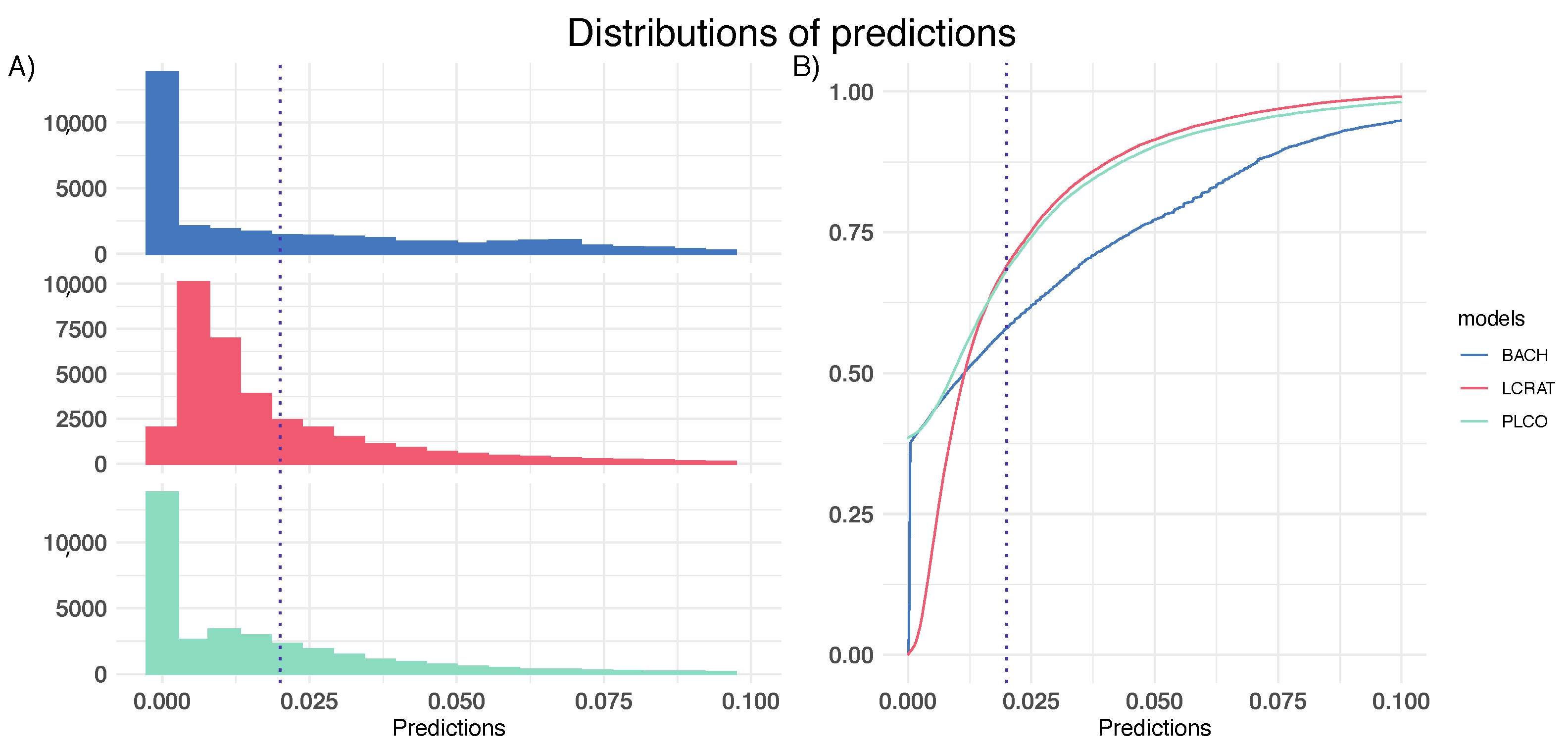
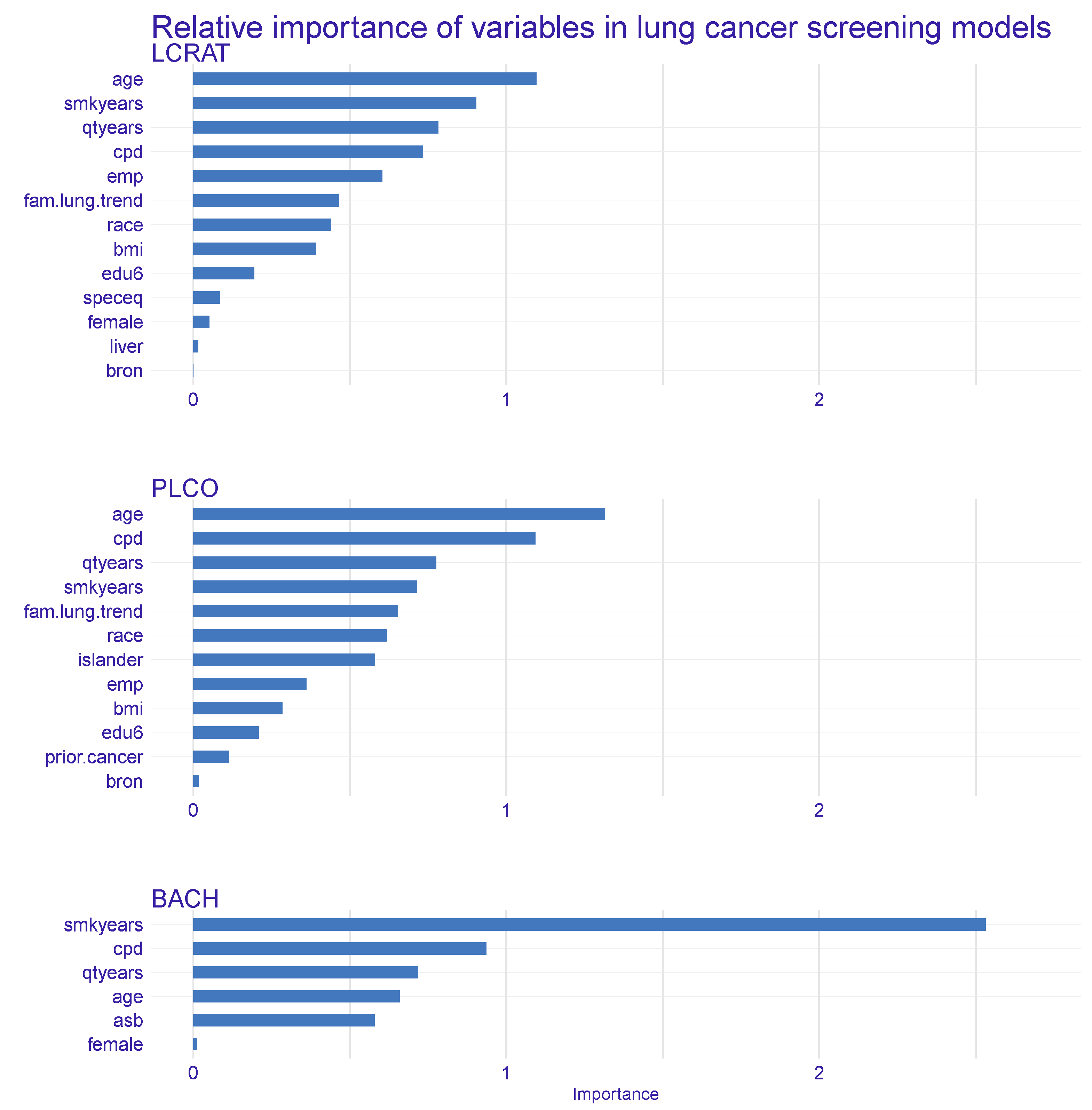
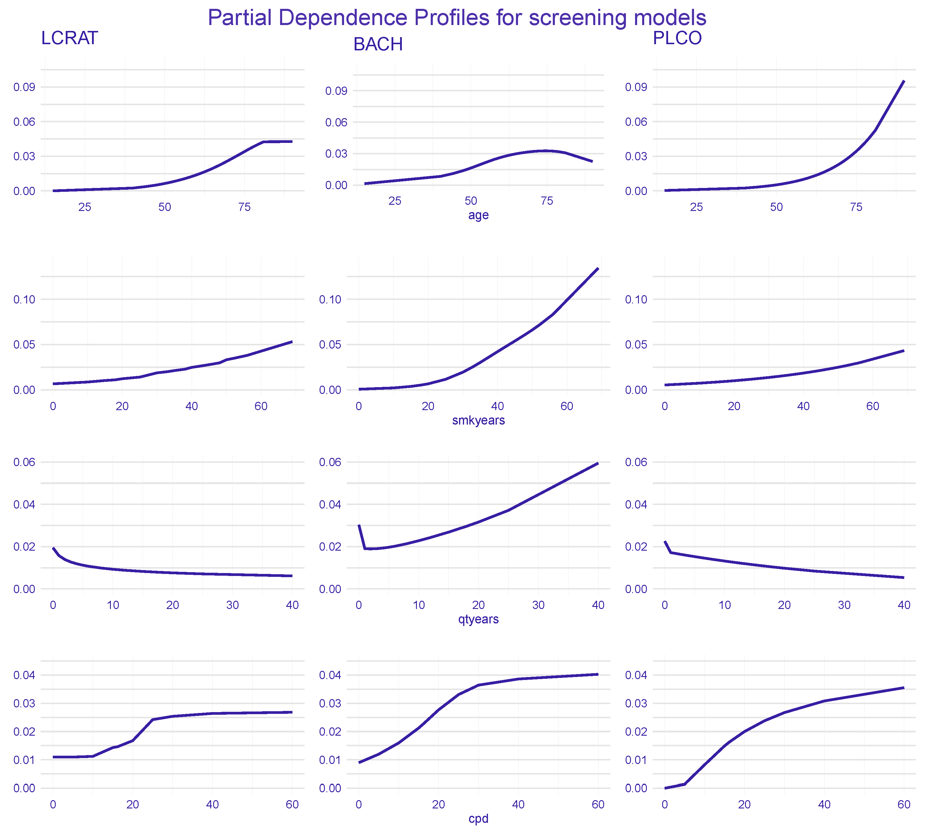
4.1. Dataset-Level Explanations

The purpose of the dataset-level explanation is to understand how the model usually behaves. We are not interested in one particular patient. The two key questions are (1) which variables are the most important and (2) how the risk prediction changes with the variable.
Figure 2 shows the importance of variables [36] in each model. First, we see that the models use different variables. For example, asbestos exposure is important for the BACH model, whereas other models do not include this factor. On the other hand, three variables (family lung trend, race, and emphysema) that are important for the LCRAT and PLCO m 2012 models are not included in the BACH model. The importance of variables from the common set is similar. The most important ones are age, number of years of smoking, cigarette count per day, and quit time. Age is the most important variable for the LCRAT and PLCO m 2012 models, but for the BACH model, it takes the fourth position. Similarly, the difference concerns years of smoking. It is the most important variable for the BACH model, whereas in the PLCO m 2012 model, it takes a lower position. According to the LCRAT model’s variable importance, years of smoking are considered the second most important (after age). However, the relative importance of these variables differs.
Figure 3 shows Partial Dependence Profiles [37,38] for the four most important variables. They summarize how the model prediction changes within the selected variable change. The greatest differences between the average models’ predictions are shown for two variables: age and smoking quit time. It is worth noticing that the considered models predict lung cancer risks for different time periods. Nevertheless, we compare the shapes of the curves rather than the absolute values of the predictions.
The PLCO m 2012 model prediction regarding age differs significantly from other models. The BACH model for the oldest people indicates counter-intuitive dependency, whereas the PLCO m 2012 model predictions increase dramatically for people more than 75 years old. For the LCRAT model, the prediction increases with age but only up to the age of 77 years. For the oldest people, the predictions remain unchanged.
Plots indicate similar dependencies between years of smoking (smkyears) and predictions for 2 models: LCRAT and PLCO m 2012 . For quitting time (qtyears), the BACH model again shows counter-intuitive dependency for the highest values. A very similar curve was also introduced in Figure 1 in the study [26]. The most similar dependencies’ partial dependence plots demonstrate for cigarettes per day variable (cpd). The BACH model prediction increases for those who smoked more than 20 years in a more radical manner than other models. Those changes among the models indicate that models exploit particular variables in different ways. It seems that some of these dependencies could be corrected.

4.2. Individual-Level Explanations

Individual-level explanations help to understand model behavior in the context of a single prediction/single patient. This perspective is much more interesting for a patient who is less interested in average behavior and most often is interested in his or her own situation. Such a local glimpse on a patient prediction can be viewed as personalized medicine. The two key questions are (1) which variables are the most important for this particular patient and (2) how the risk prediction for this patient changes with the variable.
In the current study, we focused on an observation chosen from the data. We chose a patient with the greatest disparities among the models’ predictions. The analysis was conducted for a person with a high lung cancer risk, according to the PLCO m 2012 model (over 10%), and a low risk, according to the BACH model (below 2%, which is the screening threshold). The LCRAT model indicates a risk only slightly above the threshold. Our goal was to present the main local differences between the models and point out their causes.
Figure 4 shows which variables are the most important for the selected patient. Two methods that present the contributions of local variables to the final prediction are demonstrated: (A) break down and (B) Shapley Additive Explanations (Shap). The first method presents nonadditive explanations, whereas the second one focuses only on additive explanations. The comparison of these two methodologies shows that the results of the break down [39] and Shapley attributions [5] are very similar. The only difference concerns the contribution of age equal to 90 for the BACH model. The break down plot indicates its contribution as positive, whereas Shapley indicates it as a negative contribution. In addition, comparison of the models indicates more differences. Regarding break down plots, the LCRAT and PLCO m 2012 models indicate that the patient has a high risk of lung cancer, whereas the BACH model assigns a very low prediction (lower than the 2% threshold). The most important difference between the models seems to be the contribution of quit smoking time. Only the PLCO m 2012 model suggests that being a current smoker (quit smoking value equal to zero) increases the prediction in such a significant manner. The second difference among the models is the impact of age. Age equal to 90 increases the prediction for the PLCO m 2012 and LCRAT models, whereas, according to the Bach model, age has a contribution close to zero. In fact, according to the PLCO m 2012 and LCRAT models, age is the most important variable for that patient. Cigarettes per day equal to 20 have opposite effects across the models. The LCRAT model recognizes it as a negative contributed variable, whereas the PLCO m 2012 and BACH models suggest its positive effect. It is worth noting that the BMI measure has quite a significant influence on prognosis for the LCRAT and PLCO m 2012 models, while it is not included in the BACH model.
Figure 5 illustrates how the risk prediction for the selected patient changes with the variable. Ceteris Paribus plots present the change of prediction within the change of the variable for the selected patient. The profiles indicate major differences between the PLCO m 2012 model and the two other models.
It can be observed that the variability of age, smoking years, quit time, and cigarettes per day is highest for the PLCO m 2012 model. For example, taking age into consideration, it means that if the patient was younger, the predicted risk of cancer would be much lower. The LCRAT and BACH models show much lower variation of predictions. For the selected patient, the BACH model would not change the prediction significantly, even if the patient were to quit smoking or smoke far fewer cigarettes per day.
It is also important to note that local methods present the models’ behaviors for the selected person, not for the whole cohort. Therefore, the results from local explanation methodology could be compared between the models only for the chosen patient.
The global-level explanations help to explore lung cancer risk models. These techniques give the opportunity to prepare the comparative analysis of the models. According to Figure 3, it is seen that some of the dependencies between variables and the model predictions differ drastically. It could give insight into which model is worth trusting. On the other hand, the individual-level explanations can contribute to personalized medicine. The explanations such as Ceteris Paribus, break down, and Shapley values complete each other. Such a combination of different explanation techniques could be useful and give the proper view on the model’s prediction for a selected instance.

5. Discussion and Conclusions

Lung cancer risk models are important, as they facilitate enrolling at-risk population in the screening process, thereby indirectly decreasing the mortality of one of the most common and aggressive cancers. To this end, the complex statistical risk models are increasingly used. Moreover, there are studies that compare the models in terms of the accuracy of the specific datasets, for example, ref. [31]. In our study, we fill the gap related to the interpretability of these risk models. In recent years, explainable machine learning techniques have become increasingly appreciated and are currently being widely used in different fields. The XAI methods have already been applied to lung cancer problems in [40,41]. This study presents how models that are widely recognized could be equipped with explainable machine learning techniques.
We demonstrated the approach to applying methods of explainable machine learning to three risk models. XAI methodology provides insight into the question regarding which patients’ variables are the most important. Additionally, we presented global solutions that help to understand the relationships between a particular variable and a model’s response. We believe that in the field of medicine, local explanations are even more important. Such solutions help to understand how a particular variable affects the final prognosis for a given patient. Moreover, local methods could help ascertain what can be done to change model prediction. However, local explanations can be unstable, mainly because of the underlying model being unstable. In our study, the models seems to be stable as the local explanations show smooth dependencies.
The global methods applied to screening models on the Polish database show that different models treat the dependency between some of the variables and the prediction in distinct ways. Based on the PDP method, we observed that quit smoking time, years smoked, and age have different dependencies among the models. Moreover, the Bach model indicates that years smoked are much more important than other variables. For other models, this variable’s influence does not differ in such a significant way. On the other hand, the local explaining methodology provides a wealth of information on prediction for individual patients. The local explanations presented in our study vary from each other because they are applied to three different models. Therefore, the explanation methods help us to notice the differences between those models. Overall, the local point of view is a step toward personalized medicine.

Author Contributions

Conceptualization, K.K., M.A. and P.B.; Data curation, K.K., T.O., M.A. and P.B.; Formal analysis, K.K. and P.B.; Funding acquisition, P.B.; Investigation, K.K., M.A. and P.B.; Methodology, K.K. and P.B.; Project administration, P.B.; Resources, K.K., T.O., M.A. and P.B.; Software, K.K.; Supervision, M.A. and P.B.; Validation, K.K.; Visualization, K.K.; Writing—original draft, K.K. and P.B.; Writing—review and editing, K.K., M.A. and P.B. All authors have read and agreed to the published version of the manuscript.

Funding

The article was financially supported by NCN Sonata Bis-9 grant 2019/34/E/ST6/00052 and INFOSTRATEG-I/0022/2021-00.

Institutional Review Board Statement

Not applicable.

Informed Consent Statement

Not applicable.

Data Availability Statement

Not applicable.

Conflicts of Interest

The authors declare no conflict of interest. The funders had no role in the design of the study; in the collection, analyses, or interpretation of data; in the writing of the manuscript, or in the decision to publish the results.

Appendix A

In this part, we present the mathematical formalism of explainable machine learning techniques used in the article.
To formally define explainable methods, let X = ( X 1 , . . . X n ) be a vector of variables and f : X R be a scoring function for the predictive model.

Appendix A.1. Dataset-Level Explanations

Partial Dependence Plots compute the average dependency between the variable and the prediction for all instances [42]. They summarize how the model response changes within the single variable change, presenting the marginal effect of a variable on the predicted values [38]. This method is useful for comparison of models in order to trust the final predictions. Such a comparison could assure that the model works appropriately or, on the contrary, finds the mistakes. The values on the partial dependence plot [37,38] are computed according to the following formula:
P D ( f j , z ) = E ( f ( x | j = z ) ) .
Variable’s importance indicates the most important features. It could be calculated as a drop in the model performance after randomization of a certain variable [36]. The difference between the loss function for a model and the loss function for a selected variable corresponds to its importance. Such difference could be presented as:
V I ( f , X , y ) = L o s s ( f , X , y ) L o s s ( f , X j , y )
where X j is a data with permuted j-th column.
However, there is also a possibility to compute the variable’s importance based on partial dependence plots. Then, the variable’s importance corresponds to the mean distance between Partial Dependence for a selected variable and the mean model response. This method is helpful for identification of the most important variables. Physicians can use this knowledge to validate the models with domain knowledge. Moreover, the method could lead to finding new crucial variables for a specific mechanism.
In our study, we presents the variable’s importance computed based on Partial Dependence Profiles. Let V I P D ( f , j ) be a variable importance based on the Partial Dependece Plot for function f and j-th variable. Then:
V I P D ( f , j ) = 1 n i = 1 n P D ( f , j , z i ) P D ¯ ( f , j )
where: P D ¯ ( f , j ) is a mean value of the Partial Dependence values over all values of variable j.

Appendix A.2. Individual-Level Explanations

Local-level explanations focus on the model behavior for a single observation. The break down method [39] and Shapley additive attributions [5] decompose the final prediction into contributions for a certain observation. The methodologies define which variables contribute to the final resultand in what manner. The contributions sum up to the model prediction which is the desired property of the explanation. Such methods are useful for both doctors and patients. Based on break down or Shapley additive attributions, we can learn how different variables contribute to the final prediction. However, the methods could be also useful for discovering why the model provides a wrong prediction for a specific patient. The break down for additive attribution and Shapley additive attributions divide model response into each variable contributions. For particular observation x * , the variables’ contributions v ( f , x * , i ) sum up to the model prediction:
f ( x * ) = b a s e l i n e + i = 1 p v ( f , x * , i ) .
Ceteris Paribus [8] shows the models’ possible responses if one analyzed variable would have changed, keeping all others unchanged. This method enables understanding how the oscillations of the variables influence the model prediction. Physicians might want to check which variables should be changed to improve the prediction and how, for example, in order to alert the dose of a medicine or use another therapy. Based on the Ceteris Paribus profile, a patient could understand that changing some of his features improves the prognosis, for example, a change in habits could lead to a significant prognosis change.
For a particular observation x * and the j-th variable the Ceteris Paribus [8] profile can be expressed as the following:
C P f , j , x ( z ) = f ( x | j = z )
where f ( x | j = z ) means that the value of j-th variable with changed to the z value, keeping all others unchanged for observation x.

References

  1. O’Neil, C. Weapons of Math Destruction: How Big Data Increases Inequality and Threatens Democracy; Crown Publishing Group: New York, NY, USA, 2016. [Google Scholar]
  2. European Commission. On Artificial Intelligence—A European Approach to Excellence and Trust; European Commission: Luxembourg, 2020. [Google Scholar]
  3. EU Expert Group. Ethics Guidelines for Trustworthy AI; EU Expert Group: Brussels, Belgium, 2019. [Google Scholar]
  4. Dickson, B. Inside DARPA’s Effort to Create Explainable Artificial Intelligence; DARPA: Arlington, VA, USA, 2019. [Google Scholar]
  5. Lundberg, S.M.; Lee, S.I. A Unified Approach to Interpreting Model Predictions. In Advances in Neural Information Processing Systems 30; Guyon, I., Luxburg, U.V., Bengio, S., Wallach, H., Fergus, R., Vishwanathan, S., Garnett, R., Eds.; Curran Associates, Inc.: New York, NY, USA, 2017; pp. 4765–4774. [Google Scholar]
  6. Ribeiro, M.T.; Singh, S.; Guestrin, C. “Why Should I Trust You?”: Explaining the Predictions of Any Classifier. In Proceedings of the 22nd ACM SIGKDD International Conference on Knowledge Discovery and Data Mining, San Francisco, CA, USA, 13–17 August 2016; pp. 1135–1144. [Google Scholar]
  7. Gosiewska, A.; Biecek, P. Do Not Trust Additive Explanations. arXiv 2019, arXiv:1903.11420. [Google Scholar]
  8. Biecek, P. DALEX: Explainers for Complex Predictive Models in R. J. Mach. Learn. Res. 2018, 19, 1–5. [Google Scholar]
  9. Wexler, J.; Pushkarna, M.; Bolukbasi, T.; Wattenberg, M.; Viégas, F.; Wilson, J. (Eds.) The What-If Tool: Interactive Probing of Machine Learning Models; Institute of Electrical and Electronics Engineers (IEEE): Washington, DC, USA, 2019. [Google Scholar]
  10. Nori, H.; Jenkins, S.; Koch, P.; Caruana, R. InterpretML: A Unified Framework for Machine Learning Interpretability. arXiv 2019, arXiv:1909.09223. [Google Scholar]
  11. Thorsen-Meyer, H.C.; Nielsen, A.B.; Nielsen, A.P.; Kaas-Hansen, B.S.; Toft, P.; Schierbeck, J.; Strøm, T.; Chmura, P.J.; Heimann, M.; Dybdahl, L.; et al. Dynamic and explainable machine learning prediction of mortality in patients in the intensive care unit: A retrospective study of high-frequency data in electronic patient records. Lancet Digit. Health 2020, 2, e179–e191. [Google Scholar] [CrossRef]
  12. Lundberg, S.M.; Erion, G.; Chen, H.; DeGrave, A.; Prutkin, J.M.; Nair, B.; Katz, R.; Himmelfarb, J.; Bansal, N.; Lee, S.I. From local explanations to global understanding with explainable AI for trees. Nat. Mach. Intell. 2020, 2, 56–67. [Google Scholar] [CrossRef]
  13. Hyland, S.; Faltys, M.; Hüser, M.; Lyu, X.; Gumbsch, T.; Esteban, C.; Bock, C.; Horn, M.; Moor, M.; Rieck, B.; et al. Early Prediction of Circulatory Failure in the Intensive Care Unit Using Machine Learning. Nat. Med. 2020, 26, 364–373. [Google Scholar] [CrossRef]
  14. Lundberg, S.M.; Nair, B.; Vavilala, M.S.; Horibe, M.; Eisses, M.J.; Adams, T.; Liston, D.E.; Low, D.K.W.; Newman, S.F.; Kim, J.; et al. Explainable machine-learning predictions for the prevention of hypoxaemia during surgery. Nat. Biomed. Eng. 2018, 2, 749–760. [Google Scholar] [CrossRef]
  15. Singh, A.; Sengupta, S.; Lakshminarayanan, V. Explainable Deep Learning Models in Medical Image Analysis. J. Imaging 2020, 6, 52. [Google Scholar] [CrossRef]
  16. Holzinger, A.; Biemann, C.; Pattichis, C.S.; Kell, D.B. What do we need to build explainable AI systems for the medical domain? arXiv 2017, arXiv:1712.09923. [Google Scholar]
  17. Xie, Y.; Chen, M.; Kao, D.; Gao, G.; Chen, X. CheXplain: Enabling Physicians to Explore and Understand Data-Driven, AI-Enabled Medical Imaging Analysis. In Proceedings of the CHI’20: CHI Conference on Human Factors in Computing Systems, Honolulu, HI, USA, 25–30 April 2020; Association for Computing Machinery: New York, NY, USA, 2020. [Google Scholar] [CrossRef]
  18. Lauritsen, S.M.; Kristensen, M.R.B.; Olsen, M.V.; Larsen, M.S.; Lauritsen, K.M.; Jørgensen, M.J.; Lange, J.; Thiesson, B. Explainable artificial intelligence model to predict acute critical illness from electronic health records. arXiv 2019, arXiv:1912.01266. [Google Scholar] [CrossRef]
  19. Paul, R.; Schabath, M.; Gillies, R.; Hall, L.; Goldgof, D. Convolutional Neural Network ensembles for accurate lung nodule malignancy prediction 2 years in the future. Comput. Biol. Med. 2020, 122, 103882. [Google Scholar] [CrossRef] [PubMed]
  20. Xi, J.; Zhao, W.; Yuan, J.E.; Cao, B.; Zhao, L. Multi-resolution classification of exhaled aerosol images to detect obstructive lung diseases in small airways. Comput. Biol. Med. 2017, 87, 57–69. [Google Scholar] [CrossRef] [PubMed]
  21. Li, W.; Jia, Z.; Xie, D.; Chen, K.; Cui, J.; Liu, H. Recognizing lung cancer using a homemade e-nose: A comprehensive study. Comput. Biol. Med. 2020, 120, 103706. [Google Scholar] [CrossRef] [PubMed]
  22. National Lung Screening Trial Research Team. Reduced Lung-Cancer Mortality with Low-Dose Computed Tomographic Screening. N. Engl. J. Med. 2011, 365, 395–409. [Google Scholar] [CrossRef] [Green Version]
  23. De Koning, H.J.; van der Aalst, C.M.; de Jong, P.A.; Scholten, E.T.; Nackaerts, K.; Heuvelmans, M.A.; Lammers, J.W.J.; Weenink, C.; Yousaf-Khan, U.; Horeweg, N.; et al. Reduced Lung-Cancer Mortality with Volume CT Screening in a Randomized Trial. N. Engl. J. Med. 2020, 382, 503–513. [Google Scholar] [CrossRef]
  24. Raghu, V.K.; Zhao, W.; Pu, J.; Leader, J.K.; Wang, R.; Herman, J.; Yuan, J.M.; Benos, P.V.; Wilson, D.O. Feasibility of lung cancer prediction from low-dose CT scan and smoking factors using causal models. Thorax 2019, 74, 643–649. [Google Scholar] [CrossRef] [Green Version]
  25. Tammemägi, M.C. Selecting lung cancer screenees using risk prediction models—Where do we go from here. Transl. Lung Cancer Res. 2018, 7, 243. [Google Scholar] [CrossRef]
  26. Bach, P.B.; Kattan, M.W.; Thornquist, M.D.; Kris, M.G.; Tate, R.C.; Barnett, M.J.; Hsieh, L.J.; Begg, C.B. Variations in Lung Cancer Risk Among Smokers. J. Natl. Cancer Inst. 2003, 95, 470–478. [Google Scholar] [CrossRef] [Green Version]
  27. Tammemägi, M.C.; Katki, H.A.; Hocking, W.G.; Church, T.R.; Caporaso, N.; Kvale, P.A.; Chaturvedi, A.K.; Silvestri, G.A.; Riley, T.L.; Commins, J.; et al. Selection Criteria for Lung-Cancer Screening. N. Engl. J. Med. 2013, 368, 728–736. [Google Scholar] [CrossRef] [Green Version]
  28. Katki, H.; Kovalchik, S.; Cheung, C.B.L.; Chaturvedi, A. Development and Validation of Risk Models to Select Ever-Smokers for CT Lung Cancer Screening. JAMA 2016, 315, 2300–2311. [Google Scholar] [CrossRef]
  29. R Core Team. R: A Language and Environment for Statistical Computing; R Foundation for Statistical Computing: Vienna, Austria, 2020. [Google Scholar]
  30. Cheung, L.C.; Kovalchik, S.A.; Katki, H.A. lcmodels: Predictions from Lung Cancer Models. R Package Version 4.0.0. 2019. Available online: https://dceg.cancer.gov/tools/risk-assessment/lcmodels/lcmodels-manual.pdf (accessed on 6 November 2021).
  31. Katki, H.; Kovalchik, S.; Petito, L.; Cheung, L.; Jacobs, E.; Jemal, A.; Berg, C.; Chaturvedi, A. Implications of nine risk prediction models for selecting ever-smokers for computed tomography lung cancer screening. Ann. Intern. Med. 2018, 169, 10–19. [Google Scholar] [CrossRef] [PubMed]
  32. Miller, T. Explanation in Artificial Intelligence: Insights from the Social Sciences. arXiv 2018, arXiv:1706.07269. [Google Scholar] [CrossRef]
  33. Biecek, P.; Burzykowski, T. Explanatory Model Analysis; Chapman and Hall/CRC: New York, NY, USA, 2021. [Google Scholar]
  34. Pękala, K.; Biecek, P. triplot: Explaining Correlated Features in Machine Learning Models. R Package. 2020. Available online: https://cran.r-project.org/web/packages/triplot/triplot.pdf (accessed on 6 November 2021).
  35. Apley, D. ALEPlot: Accumulated Local Effects (ALE) Plots and Partial Dependence (PD) Plots. R Package. 2018. Available online: https://cran.r-project.org/web/packages/ALEPlot/ALEPlot.pdf (accessed on 6 November 2021).
  36. Fisher, A.; Rudin, C.; Dominici, F. All Models are Wrong, but Many are Useful: Learning a Variable’s Importance by Studying an Entire Class of Prediction Models Simultaneously. J. Mach. Learn. Res. 2019, 20, 1–81. [Google Scholar]
  37. Hastie, T.; Tibshirani, R.; Friedman, J. The Elements of Statistical Learning: Data Mining, Inference, and Prediction, 2nd ed.; Springer Series in Statistics; Springer: Berlin/Heidelberg, Germany, 2009. [Google Scholar]
  38. Molnar, C. Interpretable Machine Learning. A Guide for Making Black Box Models Explainable; Leanpub: Victoria, BC, Canada, 2018. [Google Scholar]
  39. Staniak, M.; Biecek, P. Explanations of Model Predictions with live and breakDown Packages. R J. 2018, 10, 395–409. [Google Scholar] [CrossRef] [Green Version]
  40. Siddhartha, M.; Maity, P.; Nath, R. Explanatory Artificial Intelligence (XAI) in the prediction of post-operative life expectancy in lung cancer patients. Int. J. Sci. Res. 2019, 8, 112. [Google Scholar]
  41. Kobylińska, K.; Mikołajczyk, T.; Adamek, M.; Orłowski, T.; Biecek, P. Explainable Machine Learning for Modeling of Early Postoperative Mortality in Lung Cancer. In Artificial Intelligence in Medicine: Knowledge Representation and Transparent and Explainable Systems; Marcos, M., Juarez, J.M., Lenz, R., Nalepa, G.J., Nowaczyk, S., Peleg, M., Stefanowski, J., Stiglic, G., Eds.; Springer International Publishing: Cham, Switzerland, 2019; pp. 161–174. [Google Scholar]
  42. Friedman, J.H. Greedy Function Approximation: A Gradient Boosting Machine. Ann. Stat. 2000, 29, 1189–1232. [Google Scholar] [CrossRef]
Figure 1. (A) Distribution of predictions for the lung cancer risk models. (B) Cumulative distribution for three lung cancer risk models presenting the cumulative percentage of predictions. Vertical dotted lines indicate 2% threshold.
Applsci 12 01926 g001
Figure 2. Variable importance for the three considered risk models. The longer the bar is, the more important the corresponding variable. Note that asb stands for asbestos exposure, cpd stands for cigarettes per day, while islander stands for Pacific Islander ethnicity.
Applsci 12 01926 g002
Figure 3. Partial Dependence Profiles illustrate the relationship between a variable and an average model prediction. On the x-axis, the range of available values of the analyzed variable is shown, while on the y-axis, the values of the mean prediction are shown.
Applsci 12 01926 g003
Figure 4. The first column (A) presents break down plots for additive attributions. The second column (B) presents Shapley additive explanations. (A) The deep purple bar indicates the final prediction for a chosen patient. The plot also shows the contributions of each variable to the final prognosis. Green bars indicate positive contributions, meaning that the value of a certain variable implies an increase in prediction. By analogy, red bars suggest a negative contribution. The larger the bar is, the larger its contribution. (B) Green and red bars indicate the Shapley values and present the positive and negative contributions to the final prediction.
Applsci 12 01926 g004
Figure 5. Plots show the dependencies between continuous variables and the prediction for the selected patient. Blue dots indicate the real value of each variable, whereas the green lines correspond to the change of prediction with the change of the variable’s value.
Applsci 12 01926 g005
Table 1. Summary of variables used in the LCRAT, BACH, and PLCO m 2012 models. The plus sign means that the variable is included in the model.
LCRAT ModelBACH ModelPLCO m 2012 Model
Age+++
Gender++
Race/ethnicity+ +
Education+ +
BMI+ +
Smoking status +
Quitted smoking (in years)+++
Years smoked+++
Cigarettes per day+++
Pack-years+
Prior cancer +
Lung disease+ +
Asbestos exposure +
Any relatives with LC+ +
Number of relatives with LC+
Total number of variables12611
Prediction of Lung Cancer risk5 years10 years6 years
Table 2. Beta coefficients estimated in the BACH model.
VariableExpressionCoefficient
intercept −9.7960571
age  0.070322812
age 2 ( a g e 53.459001 ) 3 · I ( a g e > 53 ) ) −0.00009382122
age 3 ( a g e 61.954825 ) 3 · I ( a g e > 61 )  0.00018282661
age 4 ( a g e 70.910335 ) 3 · I ( a g e > 70 ) −0.000089005389
female −0.05827261
qtyears −0.085684793
qtyears 2 ( q t y e a r s ) 3  0.0065499693
qtyears 3 ( q t y e a r s 0.50513347 ) 3 · I ( q t y e a r s > 0 ) −0.0068305845
qtyears 4 ( q t y e a r s 12.295688 ) 3 · I ( q t y e a r s > 12 )  0.00028061519
smkyears  0.11425297
smkyears 2 ( s m k y e a r s 27.6577 ) 3 · I ( s m k y e a r s > 27 ) −0.000080091477
smkyears 3 ( s m k y e a r s 40 ) 3 · I ( s m k y e a r s > 40 )  0.00017069483
smkyears 4 ( s m k y e a r s 50.910335 ) 3 · I ( s m k y e a r s > 50 ) −0.000090603358
cpd  0.060818386
cpd 2 ( c p d 15 ) 3 · I ( c p d > 15 ) −0.00014652216
cpd 3 ( c p d 20.185718 ) 3 · I ( c p d > 20 )  0.00018486938
cpd 4 ( c p d 40 ) 3 · I ( c p d > 40 ) −0.000038347226
asbestos  0.2153936
Table 3. Descriptive statistics of continuous predictors available in the Domestic Lung Cancer Database.
VariableDescriptionMeansdMedian
ageage at diagnosis63.028.6663
smkyearssmoking years21.5918.9025
qtyearsquit smoking time1.705.030
cpdcigarettes per day13.0211.8420
Table 4. Descriptive statistics of categorical predictors available in the Domestic Lung Cancer Database.
VariableDescriptionFrequencies
femalebeing a femaleNo 0: 22,219 (64.6%)
Yes 1: 12174 (35.4%)
raceethnicityWhite 0: 34,393 (100.0%)
empemphysemaNo 0: 34,284 (99.7%)
Yes 1: 109 (0.3%)
fam.lung.trendnumber of first degree relativesNo relatives 0: 33,332 (96.9%)
with lung cancer1 or more 1: 1061 (3.1%)
asbasbestos exposureNo 0: 34,223 (99.5%)
Yes 1: 170 (0.5%)
Publisher’s Note: MDPI stays neutral with regard to jurisdictional claims in published maps and institutional affiliations.

