Computational Evaluation of Shock Wave Interaction with a Liquid Droplet

Abstract

This article represents the natural continuation of the work by Rossano and De Stefano (2021), dealing with the computational fluid dynamics analysis of a shock wave interaction with a liquid droplet. Differently from our previous work, where a two-dimensional approach was followed, fully three-dimensional computations are performed to predict the aerodynamic breakup of a spherical water body due to the impact of a traveling shock wave. The present engineering analysis focuses on capturing the early stages of the breakup process under the shear-induced entrainment regime. The unsteady Reynolds-averaged Navier–Stokes approach is used to simulate the mean turbulent flow field in a virtual shock tube device with circular cross section. The compressible-flow-governing equations are numerically solved by means of a finite volume method, where the volume of fluid technique is employed to track the air–water interface. The proposed computational modeling approach for industrial gas dynamics applications is verified by making a comparison with reference numerical data and experimental findings, achieving acceptably accurate predictions of deformation and drift of the water body without being computationally cumbersome.

1. Introduction

The aerodynamic breakup (aerobreakup) of liquid droplets into smaller fragments induced by the interaction with a passing shock wave (SW) is of crucial importance for many industrial gas dynamics applications [1,2]. These include, for example, supersonic combustion air-breathing jet engines (scramjets) and raindrop distortion and demise in the flow field around supersonic aircrafts. In the former case, mixing and combustion rates of liquid fuel droplets are greatly improved as a result of the droplet fragmentation induced by detonation waves [3]. In the latter case, erosion caused by the impingement of rain droplets at high relative speeds on aircraft surfaces, is greatly alleviated through proper aerodynamic design [4]. The shock/droplet interaction plays a very important role as it represents the initial stage of the aerobreakup induced by the high-speed gas stream. Several studies have been conducted to investigate this process for correctly interpreting the underlying physical mechanisms. In particular, a number of experimental studies employing shock tube devices have been carried out, wherein a traveling planar SW is reproduced, with uniform gaseous flow conditions being established [5,6]. In these experiments, sophisticated visualization techniques are employed, where the shock front passes over liquid droplets causing their deformation, drift and breakup, due to sudden acceleration.

Theoretically, the physics of aerobreakup is controlled by the Ohnesorge number (Oh), which compares the effects of liquid viscosity and surface tension, along with the Weber number (We), which compares disruptive aerodynamic and restorative surface tension effects. At very low Ohnesorge numbers ($\mathrm{O}\mathrm{h}\ll 1$), the influence of the liquid viscosity can be neglected so that the process is practically governed by the Weber number [7]. Previously based on a large number of different classifications of droplet crushing regimes, the interpretation and identification of the aerobreakup mechanism have been recently reviewed and greatly simplified [8]. Following this new classification, only two principal modes of fragmentation exist, according to the underlying physical mechanism of the governing interfacial instabilities. At low Weber numbers ($10<\mathrm{W}\mathrm{e}<{10}^2$), the Rayleigh–Taylor instability has to be considered the main driving mechanism for the aerobreakup, which is referred to as Rayleigh–Taylor piercing (RTP) regime. Differently, at high Weber numbers ($\mathrm{W}\mathrm{e}>{10}^3$), the breakup process is governed by the Kelvin–Helmholtz instability of the stretched liquid sheets that are formed at the periphery of the deforming droplet. This terminal regime, which is referred to as shear-induced entrainment (SIE), involves the disruption of the liquid surface layer with subsequent liquid sheet stripping and thinning, along with the spraying of stripped liquid [9].

From a numerical point of view, since the droplet aerobreakup under the SIE regime is characterized by a broad range of spatial and temporal scales, the accurate capture of the droplet deformation and fragmentation is particularly demanding in terms of computational power. Nevertheless, computational fluid dynamics (CFD) simulations have been effectively conducted to predict the early stages of the breakup process induced by the impact of a traveling SW. Due to the high computational cost of fully three-dimensional (3D) simulations, several numerical studies have dealt with two-dimensional shock/liquid column interactions [10,11,12,13,14]. In order to make them affordable, in the context of preliminary analyses, 3D computations have been most often conducted by neglecting the effects of molecular viscosity, while resolving the Euler equations [15,16]. Typically, compressible multiphase solvers based on a five-equation model [17] are used to computationally study shock/droplet interactions, where the interface between liquid and gas is modeled using volume fractions. The governing equations consist of two continuity equations for the two different phases, the mixture momentum and energy equations, and the volume fraction advection equation [16,18]. As far as turbulence modeling is concerned, either under-resolved direct numerical simulation (DNS) or large eddy simulation (LES) approaches are usually followed [6,14].

The main goal of the present work is the computational evaluation of the initial stages in the interaction process between a traveling air shock front and a water droplet following a relatively lighter approach, where the viscous effects are not neglected. Namely, the mean turbulent flow in a virtual shock tube device with circular cross section is simulated by solving the unsteady Reynolds-averaged Navier–Stokes (RANS) equations, supplied with a suitable turbulence closure model. The process is considered in the shear-stripping regime, that is, at relatively high Weber and very low Ohnesorge numbers. In this study, a 3D computational model is developed, which represents the natural extension of our previous two-dimensional work [13]. Numerical calculations are conducted by employing one of the CFD solvers that are commonly and successfully used for building virtual wind tunnels in industrial fluid dynamics research, namely, Ansys Fluent [19]. The compressible flow governing equations are solved by means of a finite volume (FV) numerical technique [12,20], where the transient tracking of the air–water interface is approximated on the fixed FV mesh by using the volume of fluid (VOF) method [21]. The present CFD modeling procedure is validated against reference data that are provided by both high-fidelity numerical solutions [15,16] and experiments [22,23].

The rest of this manuscript is organized as follows. After describing the overall computational model in Section 2, the results of the numerical simulations are presented and discussed in Section 3. Finally, in Section 4, some concluding remarks are drawn.

2. Computational Model

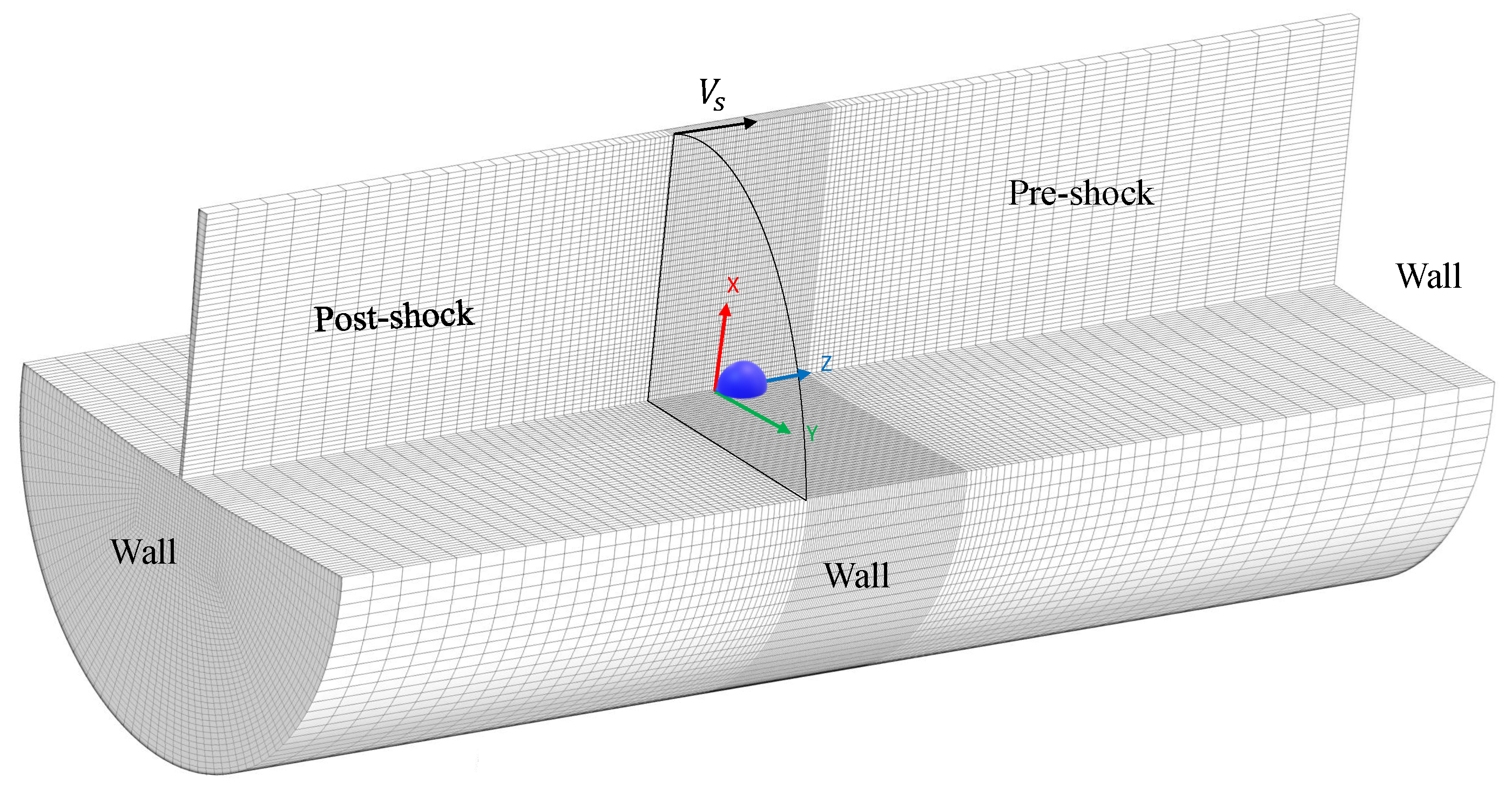
In this section, after introducing the particular industrial fluid dynamics problem under study, the details of the computational model are provided, including the method used for tracking the liquid–gas interface.

2.1. Case Study

The virtual shock tube device is built for the generation of well-defined air flow conditions to which the spherical water body is exposed. According to the 3D approach, the geometry of the shock tube is represented by the cylindrical domain sketched in Figure 1. The reference cylindrical coordinates system $(r,\theta ,z)$ is chosen with the z-axis aligned with the streamwise direction, while the origin corresponds to the leading-edge of the water droplet in its initial position. Note that the normal SW, and thus the post-shock air flow, moves in the positive z-axis direction. Furthermore, based on previous numerical simulations conducted for similar flow configurations [14], the spatial domain size is chosen such that $-21<z/d_0<26$ and $r/d_0<10$, where $d_0$ stands for the initial diameter of the spherical droplet, which represents the natural reference length of the problem.

The shock tube is divided into two parts by means of a virtual cross diaphragm, which is initially located at $z/d_0=-2$ (upstream of the droplet). In the following, the gas conditions at the right and left sides of the tube are indicated by the subscripts 1 and 4, respectively. The two tube sections are initialized with the same temperature ($T_4/T_1=1$) and very different pressure and density levels ($p_4/p_1={\rho }_4/{\rho }_1\gg 1$), with the ideal gas air being at rest on either side ($V_4=V_1=0$). Starting from these initial conditions, a normal SW develops and travels towards the driven section on the right, while a set of expansion waves propagate towards the driver section on the left. Given the pressure level $p_1$ on the right side of the tube, as well as the shock Mach number (${\mathrm{M}\mathrm{a}}_{\mathrm{s}}$) and, thus, the compression ratio across the SW, that is, $\beta =p_2/p_1$, the thermodynamic parameters to be initially imposed on the left side are analytically determined from theoretical considerations, e.g., [24]. Note that the contact surface (where $p_3=p_2$) between the two regions at different density and temperature travels at a lower velocity in the same direction as the shock.

In this study, the shock tube flow is simulated with a SW strength corresponding to ${\mathrm{M}\mathrm{a}}_{\mathrm{s}}=1.47$, which stands for the case mostly studied in the literature, starting from the pioneering experimental works of Igra and Takayama [22,23]. The actual thermodynamic parameters that are imposed as initial conditions are summarized in

Table 1. Shock tube flow parameters.

Parameter	Symbol	Value
Driven section pressure	$p_1$	101.3 kPa
Driven section density	${\rho }_1$	1.204 kg/${\mathrm{m}}^3$
Shock compression ratio	$p_2/p_1$	2.35
Driver section pressure	$p_4$	0.641 MPa
Driver section density	${\rho }_4$	7.61 kg/${\mathrm{m}}^3$
Temperature	$T_1=T_4$	293.15 K

. The air conditions in the driven section correspond to atmospheric pre-shock conditions, while the ambient conditions imposed to the air surrounding the water droplet, which are indicated by the subscript 2, correspond to the high-speed stream behind the shock.

These conditions, together with the droplet parameters, are provided in

Table 2. Post-shock air flow and water body parameters.

Parameter	Symbol	Value
Air temperature	$T_2$	381 K
Air density	${\rho }_2$	2.18 kg/${\mathrm{m}}^3$
Air viscosity	${\mu }_2$	2.23 × 10${}^{-5}$ Pa/s
Air velocity	$V_2$	225.9 m/s
Shock front velocity	$V_{\mathrm{S}}$	504.5 m/s
Droplet diameter	$d_0$	4.80 × 10${}^{-3}$ m
Water density	${\rho }_{l0}$	998 kg/${\mathrm{m}}^3$
Water viscosity	${\mu }_{l0}$	1.003 × 10${}^{-3}$ Pa/s
Surface tension	$\sigma$	7.286 × 10${}^{-2}$ N/m

, where $V_{\mathrm{S}}$ represents the constant velocity of the traveling SW front. Note that, given the present post-shock thermodynamic conditions, the ambient pressure results in being greater than the saturation pressure of water. This way, the liquid body does not undergo phase change and the two different fluids can be considered immiscible. It is worth stressing that the above condition could be no more valid for increasing Mach number.

The compressible aerodynamics of the problem under investigation is governed by the flow’s Mach and Reynolds numbers at free-stream conditions, defined as

$$\mathrm{M}\mathrm{a}=\frac{V_2}{\sqrt{\gamma p_2/{\rho }_2}},$$

(1)

and

$$\mathrm{R}\mathrm{e}=\frac{{\rho }_2{V}_2{d}_0}{{\mu }_2},$$

(2)

respectively. Moreover, as discussed in the previous section, the droplet aerobreakup induced by the SW impact is controlled by the Ohnesorge number for the liquid droplet,

$$\mathrm{O}\mathrm{h}=\frac{{\mu }_{l0}}{\sqrt{{\rho }_{l0}\sigma d_0}},$$

(3)

which is based on the water properties, and the Weber number,

$$\mathrm{W}\mathrm{e}=\frac{{\rho }_2{V}_2^2{d}_0}{\sigma },$$

(4)

which is based on the post-shock air conditions. The constant surface tension $\sigma$ at the air–water interface appearing in both definitions (3) and (4) is assumed constant. In addition, the droplet-phase-to-ambient-phase density ratio, $\epsilon ={\rho }_{l0}/{\rho }_2$, and droplet-phase-to-ambient-phase viscosity ratio, $N={\mu }_{l0}/{\mu }_2$, are usually taken into account.

Basically, the size of the liquid droplet plays a crucial role in determining both the air flow regime and the droplet breakup characteristics. The current value for the initial droplet diameter, that is, $d_0=4.8$ mm, corresponding to the classical reference experiments [22,23], has been widely used in numerical investigations of the aerobreakup in the SIE regime [10,15]. Based on this reference length and the other physical parameters that are involved in their definitions, the above-mentioned characteristic dimensionless groups take the values provided in

Table 3. Characteristic dimensionless groups.

Group	Symbol	Value
Mach number	$\mathrm{M}\mathrm{a}$	$0.577$
Reynolds number	$\mathrm{R}\mathrm{e}$	$1.06\times {10}^5$
Ohnesorge number	$\mathrm{O}\mathrm{h}$	$1.64\times {10}^{-4}$
Weber number	$\mathrm{W}\mathrm{e}$	$7.33\times {10}^3$
Density ratio	$\epsilon$	459
Viscosity ratio	N	$44.9$

.

Owing to the very low Ohnesorge and the relevant Weber numbers, the current aerobreakup configuration does belong to the SIE regime, where the gas is expected to go around the liquid mass producing a surface layer peeling-and-ejection action [25]. Capillary effects could be neglected with respect to the inertial ones in the early stages of the aerodynamic breakup, where shear stripping is the dominant mechanism. Furthermore, based on the relatively high Reynolds number, viscous effects could be considered negligible. In fact, differently from this work, several numerical investigations of the droplet aerobreakup have been conducted by solving the compressible Euler equations in absence of surface tension [15].

2.2. CFD Analysis

The present engineering analysis employed the compressible Navier–Stokes equations, by also considering the surface tension effects at the air–water interface.

2.2.1. VOF Method

For the transient tracking of the liquid–gas interface during the interaction process, the VOF method was used, which allows the approximation of the boundary between the two different phases on a fixed numerical mesh. The VOF technique was shown to be more efficient and flexible than other methods when treating the complex interface between two immiscible fluids [21], and has been very often employed to study the SW/droplet interaction [6,12].

Practically, the compressible Navier–Stokes equations are written for volume-averaged fields that are shared by the two different phases. The governing equations are solved for an effective fluid, whose averaged properties are evaluated according to the volume fractions. For example, the averaged density and viscosity are determined by:

$$\rho =\alpha {\rho }_l+(1-\alpha ){\rho }_g$$

(5)

and

$$\mu =\alpha {\mu }_l+(1-\alpha ){\mu }_g,$$

(6)

where ${\rho }_g$ and ${\mu }_g$ correspond to the gaseous phase, while $\alpha$ stands for the volume fraction of liquid water. The flow field variable $\alpha$ is evaluated throughout the computational domain by solving the corresponding continuity equation, while the volume fraction of the ideal gas is plainly computed. In any computational cell, depending on the local volume fractions, the fluid properties and the flow variables are representative of either one of the two phases ($\alpha =0$ or $\alpha =1$) or a mixture of them in the transitional regions ($0<\alpha <1$). In the following presentation of the results, the air/liquid interface is assumed to correspond to the isosurface at $\alpha =0.5$ for the liquid volume fraction. Note that, due to the explicit formulation that was adopted to compute the time-dependent VOF solution, the time step size was practically limited by stability constraints. Furthermore, the sharp interface modeling type, along with interfacial antidiffusion, was used [16].

Finally, one of the advantages of the VOF method is that the effect of surface tension forces at the air–water interface can be simply simulated. Specifically, the present analysis for the SW/droplet interaction was carried out by employing the continuum surface force (CSF) model proposed in [26], with the momentum equation being supplied with an additional source term due to surface tension [18].

2.2.2. CFD Solution

The mean turbulent flow in the virtual shock tube device was simulated by solving the unsteady compressible RANS equations. The shear-stress transport (SST) k–$\omega$ two-equation eddy-viscosity model was used for turbulence closure, owing to its proven suitability for complex fluids engineering applications [27]. The flow governing equations, which are not reported here for brevity, can be found, for instance, in [28]. The numerical simulations were performed by using the industrial solver Ansys Fluent, which has been successfully employed in analogous works [13,19], as well as in previous CFD studies using RANS models by the same research group [29,30].

The present pressure-based solver utilized the FV approach to discretize the governing equations and approximate the unsteady mean flow solution, where the conservation principles were applied over each computational cell [31,32]. The FV grid was suitably refined in the flow region, just ahead of the diaphragm, that is interested by the SW formation and occupied by the deforming water body, including the near wake, as sketched in Figure 1. Moreover, in order to save computing power, the computational domain that was used corresponded to half the cylindrical shock tube domain, namely $y\ge 0$, where a symmetry boundary condition was imposed at the centerplane. In fact, according to previous experimental visualizations, the flow can be assumed symmetric at the early stages of the interaction process [22]. Wall boundary conditions were employed for simulating the solid walls of the virtual shock tube device, as was done in similar studies, e.g., [12]. The second-order upwind scheme was used for spatial discretization, while the constant time-step of $\mathsf{\Delta }t=2\times {10}^{-7}$ s was used for the explicit transient calculation.

A grid sensitivity analysis was performed by examining the shock front and the post-shock velocities predicted using three different FV grids with increasing resolution, as reported in

Table 4. Shock tube flow: traveling velocities for different mesh resolutions.

Solution	# of FV Cells	${\mathit{h}}_{\mathit{m}\mathit{i}\mathit{n}}/{\mathit{d}}_0$	${\mathit{V}}_{\mathbf{S}}$ (m/s)	${\mathit{V}}_2$ (m/s)
CFD I	$6.5\times {10}^6$	$3.4\times {10}^{-2}$	$504.1$	$225.6$
CFD II	$9\times {10}^6$	$2.5\times {10}^{-2}$	$504.3$	$225.7$
CFD III	$15\times {10}^6$	$1.1\times {10}^{-2}$	$504.4$	$225.8$
Analytical	−	−	$504.5$	$225.9$

. Therein, $h_{min}$ stands for the minimum characteristic mesh size, which was evaluated as the cubic root of the cell volume. The total number of FV elements ranged between $6.5$ and 15 million, where the finest local resolution resulted in 90 cells per original droplet diameter.

The system of integral balance equations for mass, momentum, and energy was completed by employing two equations of state to model the density variations of the two different fluids. Specifically, along with the ideal gas law for the gaseous phase, the following equation of state for the liquid phase was considered [33],

$$\frac{{\rho }_l}{{\rho }_{l0}}={\left(\frac{p+\mathcal{B}}{p_0+\mathcal{B}}\right)}^{\frac{1}{\kappa }},$$

(7)

where $p_0$ and ${\rho }_{l0}$ represent the reference pressure and density levels, while $\mathcal{B}$ and $\kappa$ are constant parameters. Following [12], the pressure-like parameter $\mathcal{B}$ and the so-called adiabatic index $\kappa$ were set to the values of 305 MPa and $6.68$, respectively. However, given the maximum pressure level expected in the simulations, the liquid density can be considered practically constant for the present engineering analysis.

3. Results

The computational setup described in Section 2.1, without the presence of the water droplet, practically corresponds to the classical shock tube problem [34], which admits an exact inviscid solution and has become a standard test case for compressible flow solvers. Therefore, while demonstrating the post-shock air flow in which the liquid droplet is immersed, the initial simulation of the empty shock tube device also represents a preliminary verification and validation test to be completed, e.g., [10].

Here, the robustness of the present CFD model and the accuracy of the transient numerical solution of the shock tube problem were assessed through comparison with the corresponding analytical discontinuous solution [24]. Specifically, the profiles along the shock tube of different flow field variables at a time instant, say $t_0=2d_0/V_{\mathrm{S}}$, when the incident shock impacts the droplet, were examined. By looking at the pressure, temperature, density and velocity plots that are reported in Figure 2, for the three different mesh resolutions, the comparison between numerical and analytical solutions is quite satisfactory. Note that, as it happens in real flows, theoretical discontinuities are smoothed out by resolving viscous effects in practical simulations. Based on the present grid sensitivity analysis, as well as other similar studies using the VOF methodology, the spatial resolution associated with the solution CFD III can be assumed fully adequate to capture the salient flow features without being computationally cumbersome.

The above preliminary simulation allows us to confirm the overall characteristics of the case study described in Section 2.1. In particular, the expansion waves are demonstrated to travel in the opposite direction with respect to the shock front and thus, do not influence the SW/droplet interaction. Subsequently, the complete setup was employed to simulate the interaction of a single water droplet with a traveling SW, where distortion and successive breakup of the water body are observed, as a consequence of the impact of the shock front. In the following discussion, as is usually done in the relevant literature [2,7], the following nondimensional group

$$t^{*}=\frac{V_2}{d_0\sqrt{\epsilon }}(t-t_0)$$

(8)

was used as normalized time variable for examining the droplet aerobreakup.

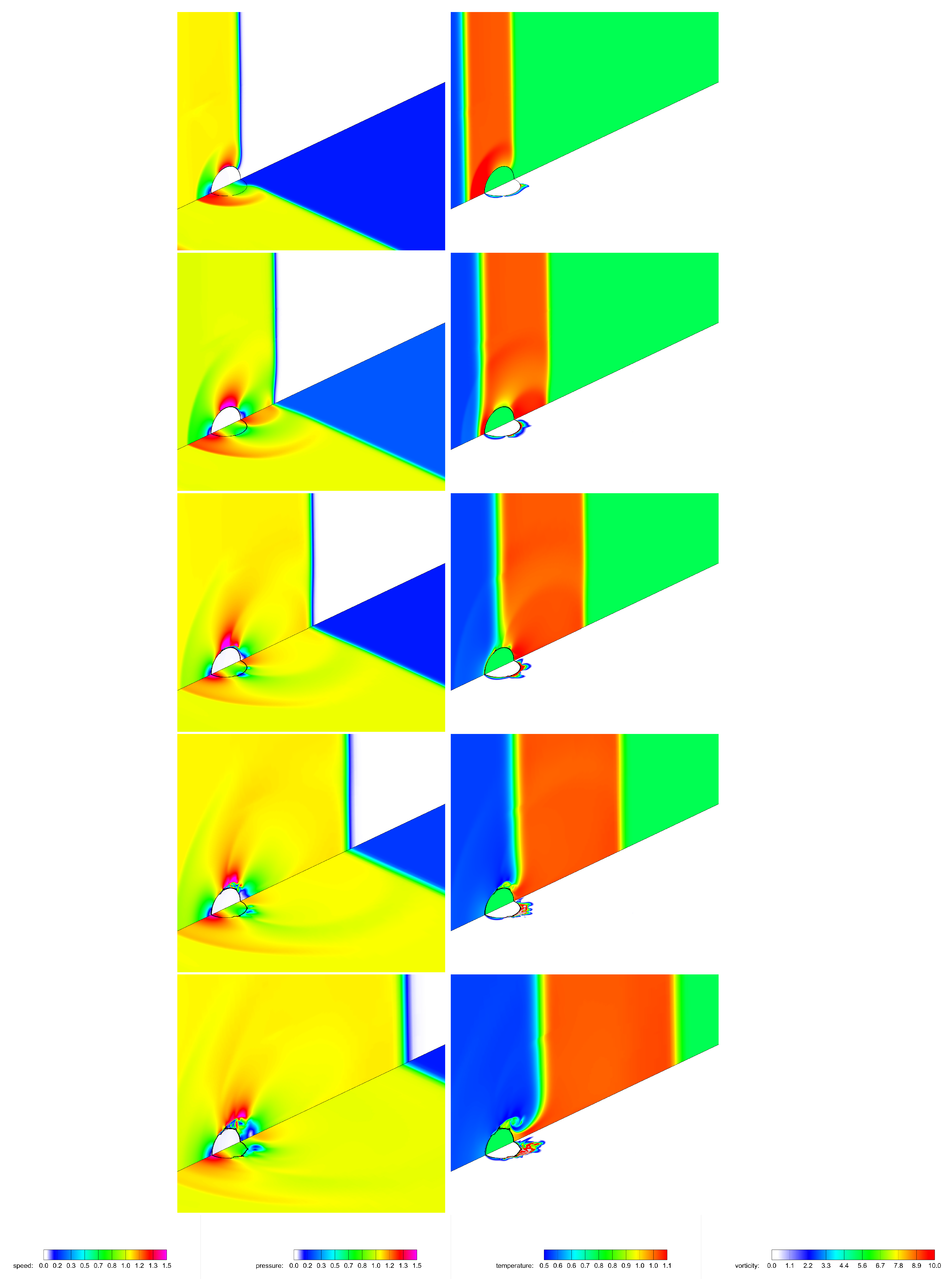
3.1. Qualitative Analysis

The early stages of the interaction process are illustrated in Figure 3, by considering the temporal evolution of the air–water interface, immediately after the SW impact. The snapshots correspond to twelve different time instants in the interval $0<t^{*}\le 0.72$, as they are indicated in the instantaneous pictures, where both front and back views are reported. Here and in the following, the instantaneous shape of the deforming droplet is determined as that one associated with the isosurface at $\alpha =0.5$ for the volume fraction of water. Note that, to correctly visualize the deformation of the water body, the size and position of the zoomed images are exactly the same for each snapshot. Moreover, due to the adopted numerical resolution, the interface between the two immiscible fluids appears to be very slightly diffuse.

As it is apparent from these pictures, initially, the passage of the SW does not produce appreciable droplet deformation. There exists a reaction time, which depends on both drop size and air stream velocity [35], during which the water body appears undistorted, with the air flow field practically resembling the flow past a rigid sphere. As the interaction process continues, after the reaction time has elapsed, small-scale instabilities on the liquid droplet surface appear. The droplet begins to be distorted due to the dominant action of the shock-induced pressure gradient along the axial direction, while still maintaining its coherence. The windward side of the water body remains practically spherical, while the leeward side is flattened into a planar surface, which corresponds to a decreasing axial width. At the same time, the droplet is dragged by the air stream moving at high velocity, while the liquid starts to be stripped at the droplet’s equator. In fact, according to the sheet thinning mechanism proposed by Liu and Reitz [36], the thin liquid sheet being drawn off at the droplet periphery is accelerated and stretched by the dominant action of shear forces due to the surrounding air flow. The liquid sheet becomes thinner and thinner until, eventually, flow instability leads to its incipient breakup into ligaments and the generation of small product droplets. As illustrated in the figure, the parent droplet is continually flattened in the streamwise direction and eroded at the periphery, with the entrainment of small droplets from the liquid sheet edge, near the equator of the main water body. Basically, these pictures confirm the qualitative characteristics of the shear-stripping breakup mechanism, as is expected at the present high Weber number [25]. During the successive stages, the droplet would disintegrate into fragments distributed widely in the flow field, which is out of the scope of this study.

In order to illustrate the resolved mean flow, in Figure 4 and Figure 5, the instantaneous contour maps for some variables of interest are reported. On the left column of these figures, the vertical plots show the speed that is the modulus of the velocity vector, while the horizontal plots show the pressure field, normalized by the corresponding post-shock values that are $V_2$ and $p_2$. On the right column, the vertical plots show the temperature field, normalized by $T_2$, while the horizontal plots show the vorticity magnitude field, normalized by $V_2/d_0$. All these two-dimensional slices are taken through the original center of the droplet, at the plane $x=0$, while a rotation is performed for graphical purposes, with the positive z-axis direction being from the bottom left to top right corners. The different instantaneous pictures are ordered from top to bottom. Furthermore, the initial position of the droplet is represented in the vertical planes to highlight the movement and deformation induced by the SW interaction.

By inspection of the snapshots in Figure 4, corresponding to the time interval $0.01\le t^{*}\le 0.17$, during which the water body changes in shape very slightly, both incident and reflected moving wave fronts are evident, as well as the transmitted wave inside the water body [12]. Immediately after the passage of the main shock, the air flow is accelerated so that the speed approximately becomes $1.5V_2$ at the droplet’s equator, which is the exact value for potential flow past a rigid sphere. As it is clearly illustrated in Figure 5, corresponding to the time interval $0.25\le t^{*}\le 0.65$, during the early stages of the interaction process, the droplet flattening is a consequence of the nonuniform pressure distribution around the droplet surface, with high pressures at the forward and rear stagnation regions and low pressures at the equator, which is due to the acceleration of the surrounding gas. Furthermore, as it is illustrated by the temperature contour maps, the liquid phase is practically maintained at the constant temperature corresponding to the initial conditions.

It is worth stressing that the above qualitative analysis for the initial stages of the interaction process, in terms of unsteady mean flow variables, is fully consistent with the results provided by more sophisticated high-fidelity numerical simulations performed at the same Mach number [15], as well as the experimental visualizations of the SIE phenomenology [37]. In particular, differently from the classical description of the breakup process as corresponding to two consecutive stages [36], the present CFD study confirms that droplet flattening and stripping of liquid material from the parent body occur simultaneously, while being complexly connected, as was already observed in [15].

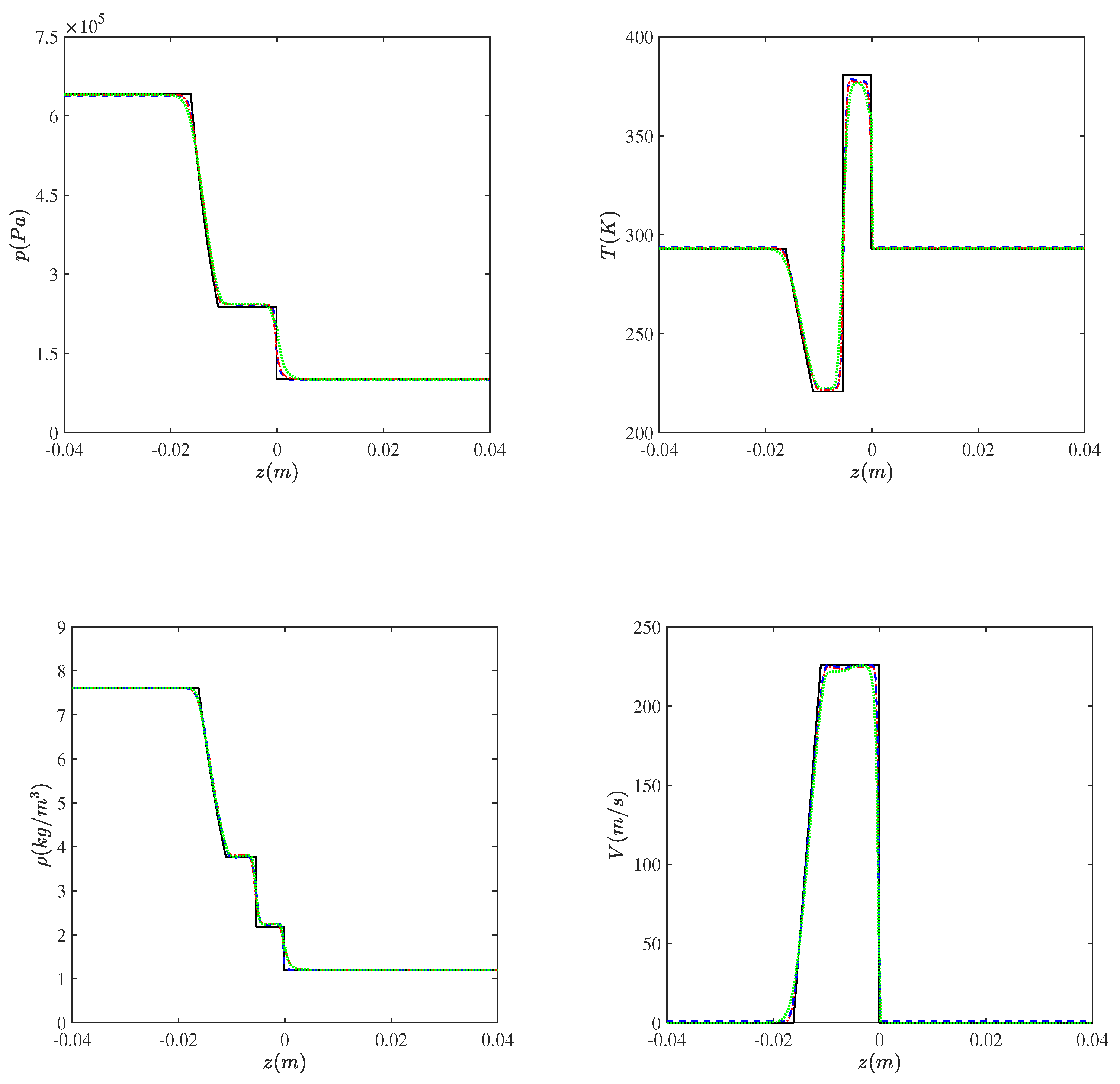
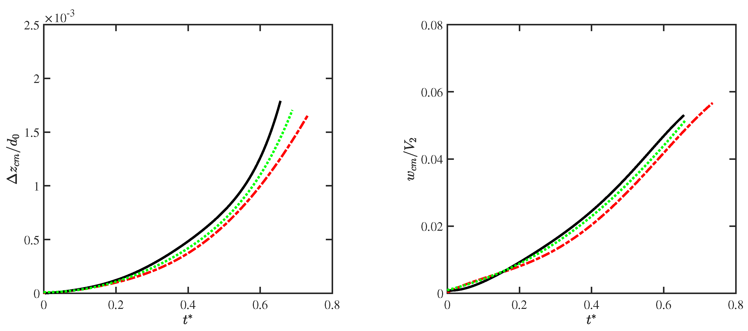
3.2. Quantitative Validation

The quantitative validation of the proposed CFD model was performed by examining the movement and deformation of the water droplet against time, while making a comparison with reference numerical data [15,16]. The time-dependent axial position of the center-of-mass (CM) of the water droplet is simply determined by:

$$z_{\mathrm{CM}}=\frac{{\int }_{\Omega }\alpha {\rho }_{l}zd\Omega }{{\int }_{\Omega }\alpha {\rho }_{l}d\Omega },$$

(9)

where $\Omega$ represents the overall computational domain. Analogously, the axial velocity of the droplet CM is given by:

$$w_{\mathrm{CM}}=\frac{{\int }_{\Omega }\alpha {\rho }_{l}wd\Omega }{{\int }_{\Omega }\alpha {\rho }_{l}d\Omega }.$$

(10)

Owing to the VOF formulation, the above equations inherently exclude the contribution from the flow region that is actually occupied by the gaseous phase ($\alpha =0$).

By inspection of Figure 6, wherein the time histories of the CM drift and velocity are given for two different FV grid resolutions, the present CFD data appear to be acceptably accurate when compared to high-fidelity numerical results [15]. In practice, the present engineering analysis provides slightly anticipated movement and deformation of the liquid droplet. However, since the above integral parameters result in being quite insensitive to small-scale interface structures, which are not resolvable by means of the current mean flow analysis, the overall movement of the droplet is satisfactorily captured. Furthermore, the positive effect of increasing the mesh resolution is apparent.

Furthermore, the streamwise acceleration $a_{\mathrm{cm}}$ of the droplet CM was obtained by differentiating the discrete velocity data using second-order finite difference approximations, for both the present CFDs and reference numerical solutions [13]. Looking at the time evolution of this variable, which is reported suitably normalized on the left side of Figure 7, the good agreement with reference data in [15] is confirmed. Note that a similar result also holds for the aerodynamic drag coefficient of the water body. As to the droplet deformation, the time history of the decreasing axial width d, normalized by the initial diameter $d_0$, is shown on the right side of Figure 7. Apparently, an acceptable agreement is achieved between the present solution and reference numerical data in [16], where the Mach number is almost the same, with the comparison improving for increasing resolution.

It is worth stressing that both reference numerical simulations were conducted without considering the effects of molecular viscosity and surface tension. In particular, the finest mesh resolution that was used in [15] corresponded to 100 cells per original droplet diameter, while no modeling procedure was introduced for the residual unresolved flow scales. Therefore, that solution can be interpreted as either under-resolved DNS or no-model LES, where the numerical scheme inherently included artificial viscosity. Differently, the present study aims to investigate the mean flow by solving the unsteady RANS equations supplied with a suitable closure model.

Finally, based on the acceptable results that were obtained in terms of both qualitative analysis and quantitative validation with respect to reference numerical and experimental findings, the proposed CFD model was shown to be able to capture the salient features of this particular industrial fluid dynamics application, without being computationally cumbersome. This highlights the benefits of the present relatively simple and straightforward numerical approach.

4. Conclusions

This study was intended as a proof of concept, namely the preliminary development and demonstration of an industrial CFD-based prediction methodology to simulate the distortion and breakup of water droplets induced by the passage of a normal SW. Following the unsteady compressible RANS approach, a CFD analysis of the early stages of the droplet aerobreakup, under the shear-stripping regime, was performed. The use of a virtual wind tunnel allowed us to reproduce post-shock flow conditions, as well as droplet distortion and incipient breakup features observed in experiments conducted in real shock tube devices. Both coexistent features of the process, which are water droplet flattening and sheet shearing at the droplet’s equator, were reproduced with acceptable accuracy. The presented results were in good agreement, both qualitatively and quantitatively, with reference solutions provided by high-fidelity numerical studies.

Finally, there remains the possibility of developing more sophisticated computational methodologies for this particular gas dynamics application, depending on the level of accuracy that is desired and the computational cost that is affordable. For instance, following [18], a wavelet-based adaptive multiscale approach could be followed [38,39]. This innovative methodology, which exploits the wavelet transform to dynamically and automatically adjust the grid resolution to the local flow conditions, has recently been further developed for wall-bounded supersonic flows [40,41]. In particular, wavelet-based adaptive unsteady RANS models [42,43,44] could be explored in the present context. Moreover, in order to simulate the appearance and dynamics of microdroplets during the later stages of the process, hybrid VOF-Lagrangian methods [45] could be developed in this framework [46].

References

1. Villermaux, E. Fragmentation. Annu. Rev. Fluid Mech. 2007, 39, 419–446. [Google Scholar] [CrossRef]
2. Nicholls, J.A.; Ranger, A.A. Aerodynamic shattering of liquid drops. AIAA J. 1969, 7, 285–290. [Google Scholar] [CrossRef]
3. Benjamin, M.A.; Jensen, R.J.; Arienti, M. Review of atomization: Current knowledge and future requirements for propulsion combustors. At. Sprays 2010, 20, 485–512. [Google Scholar] [CrossRef]
4. Moylan, B.; Landrum, B.; Russell, G. Investigation of the physical phenomena associated with rain impacts on supersonic and hypersonic flight vehicles. Procedia Eng. 2013, 58, 223–231. [Google Scholar] [CrossRef] [Green Version]
5. Wang, Z.; Hopfes, T.; Giglmaier, M.; Adams, N.A. Effect of Mach number on droplet aerobreakup in shear stripping regime. Exp. Fluids 2020, 61, 193. [Google Scholar] [CrossRef] [PubMed]
6. Poplavski, S.; Minakov, A.; Shebeleva, A.; Boiko, V. On the interaction of water droplet with a shock wave: Experiment and numerical simulation. Int. J. Multiph. Flow 2020, 127, 103273. [Google Scholar] [CrossRef]
7. Guildenbecher, D.R.; López-Rivera, C.; Sojka, P.E. Secondary atomization. Exp. Fluids 2009, 46, 371–402. [Google Scholar] [CrossRef]
8. Theofanous, T.G.; Li, G.; Dinh, T.N. Aerobreakup in rarefied supersonic gas flows. Trans. ASME J. Fluid Eng. 2004, 126, 516–527. [Google Scholar] [CrossRef]
9. Theofanous, T.G.; Li, G. On the physics of aerobreakup. Phys. Fluids 2008, 20, 052103. [Google Scholar] [CrossRef]
10. Chen, H. Two-dimensional simulation of stripping breakup of a water droplet. AIAA J. 2008, 46, 1135. [Google Scholar] [CrossRef]
11. Meng, J.C.; Colonius, T. Numerical simulations of the early stages of high-speed droplet breakup. Shock Waves 2015, 25, 399–414. [Google Scholar] [CrossRef]
12. Sembian, S.; Liverts, M.; Tillmark, N.; Apazidis, N. Plane shock wave interaction with a cylindrical water column. Phys. Fluids 2016, 28, 056102. [Google Scholar] [CrossRef]
13. Rossano, V.; De Stefano, G. Computational evaluation of shock wave interaction with a cylindrical water column. Appl. Sci. 2021, 11, 4934. [Google Scholar] [CrossRef]
14. Nykteri, G.; Gavaises, M. Droplet aerobreakup under the shear-induced entrainment regime using a multiscale two-fluid approach. Phys. Rev. Fluids 2021, 6, 084304. [Google Scholar] [CrossRef]
15. Meng, J.C.; Colonius, T. Numerical simulation of the aerobreakup of a water droplet. J. Fluid Mech. 2018, 835, 1108–1135. [Google Scholar] [CrossRef] [Green Version]
16. Liu, N.; Wang, Z.; Sun, M.; Wang, H.; Wang, B. Numerical simulation of liquid droplet breakup in supersonic flows. Acta Astronaut. 2018, 145, 116–130. [Google Scholar] [CrossRef]
17. Allaire, G.; Clerc, S.; Kokh, S. A five-equation model for the simulation of interfaces between compressible fluids. J. Comput. Phys. 2002, 181, 577–616. [Google Scholar] [CrossRef] [Green Version]
18. Hosseinzadeh-Nik, Z.; Aslani, M.; Owkes, M.; Regele, J.D. Numerical simulation of a shock wave impacting a droplet using the adaptive wavelet-collocation method. In Proceedings of the ILASS-Americas 28th Annual Conference on Liquid Atomization and Spray Systems, Dearborn, MI, USA, 15–18 May 2016. [Google Scholar]
19. Anderson, M.; Vorobieff, P.; Truman, C.R.; Corbin, C.; Kuehner, G.; Wayne, P.; Conroy, J.; White, R.; Kumar, S. An experimental and numerical study of shock interaction with a gas column seeded with droplets. Shock Waves 2015, 25, 107–125. [Google Scholar] [CrossRef]
20. De Stefano, G.; Denaro, F.M.; Riccardi, G. High-order filtering for control volume flow simulation. Int. J. Numer. Methods Fluids 2001, 37, 797–835. [Google Scholar] [CrossRef]
21. Hirt, C.W.; Nichols, B.D. Volume of fluid (VOF) method for the dynamics of free boundaries. J. Comput. Phys. 1981, 39, 201–225. [Google Scholar] [CrossRef]
22. Igra, D.; Takayama, K. Investigation of aerodynamic breakup of a cylindrical water droplet. At. Sprays 2001, 11, 167–185. [Google Scholar]
23. Igra, D.; Takayama, K. Experimental investigation of two cylindrical water columns subjected to planar shock wave loading. J. Fluids Eng. 2003, 125, 325–331. [Google Scholar] [CrossRef]
24. Laney, C.B. Computational Gasdynamics; Cambridge University Press: Cambridge, UK; New York, NY, USA, 1998. [Google Scholar]
25. Theofanous, T.G. Aerobreakup of Newtonian and viscoelastic liquids. Annu. Rev. Fluid Mech. 2011, 43, 661–690. [Google Scholar] [CrossRef]
26. Brackbill, J.U.; Kothe, D.B.; Zemach, C. A continuum method for modeling surface tension. J. Comput. Phys. 1992, 100, 335–354. [Google Scholar] [CrossRef]
27. Menter, F.R. Two-equation eddy-viscosity turbulence models for engineering applications. AIAA J. 1994, 32, 1598–1605. [Google Scholar] [CrossRef] [Green Version]
28. Wilcox, D.C. Turbulence Modelling for CFD, 3rd ed.; DCW Industries, Inc.: La Canada, CA, USA, 2006. [Google Scholar]
29. De Stefano, G.; Natale, N.; Reina, G.P.; Piccolo, A. Computational evaluation of aerodynamic loading on retractable landing-gears. Aerospace 2020, 7, 68. [Google Scholar] [CrossRef]
30. Natale, N.; Salomone, T.; De Stefano, G.; Piccolo, A. Computational evaluation of control surfaces aerodynamics for a mid-range commercial aircraft. Aerospace 2020, 7, 139. [Google Scholar] [CrossRef]
31. Iannelli, P.; Denaro, F.M.; De Stefano, G. A deconvolution-based fourth-order finite volume method for incompressible flows on non-uniform grids. Int. J. Numer. Methods Fluids 2003, 43, 431–462. [Google Scholar] [CrossRef]
32. Denaro, F.M.; De Stefano, G. A new development of the dynamic procedure in large-eddy simulation based on a Finite Volume integral approach. Application to stratified turbulence. Theor. Comput. Fluid Dyn. 2011, 25, 315–355. [Google Scholar] [CrossRef]
33. Shyue, K.M. A fluid-mixture type algorithm for barotropic two-fluid flow problems. J. Comput. Phys. 1998, 200, 718–748. [Google Scholar] [CrossRef]
34. Sod, G.A. A survey of several finite difference methods for systems of nonlinear hyperbolic conservation laws. J. Comput. Phys. 1978, 27, 1–31. [Google Scholar] [CrossRef] [Green Version]
35. Engel, O.G. Fragmentation of waterdrops in the zone behind an air shock. J. Res. Natl. Bur. Stand. 1958, 60, 245–280. [Google Scholar] [CrossRef]
36. Liu, Z.; Reitz, R.D. An analysis of the distortion and breakup mechanisms of high speed liquid drops. Int. J. Multiph. Flow 1997, 23, 631–650. [Google Scholar] [CrossRef]
37. Theofanus, T.G.; Mitkin, V.V.; Ng, C.L.; Chang, C.H.; Deng, X.; Sushchikh, S. The physics of aerobreakup. II. Viscous liquids. Phys. Fluids 2012, 24, 022104. [Google Scholar] [CrossRef]
38. De Stefano, G.; Vasilyev, O.V. Hierarchical adaptive eddy-capturing approach for modeling and simulation of turbulent flows. Fluids 2021, 6, 83. [Google Scholar] [CrossRef]
39. Ge, X.; De Stefano, G.; Hussaini, M.Y.; Vasilyev, O.V. Wavelet-based adaptive eddy-resolving methods for modeling and simulation of complex wall-bounded compressible turbulent flows. Fluids 2021, 6, 331. [Google Scholar] [CrossRef]
40. De Stefano, G.; Brown-Dymkoski, E.; Vasilyev, O.V. Wavelet-based adaptive large-eddy simulation of supersonic channel flow. J. Fluid Mech. 2020, 901, A13. [Google Scholar] [CrossRef]
41. Kasimov, N.; Dymkoski, E.; De Stefano, G.; Vasilyev, O.V. Galilean-invariant characteristic-based volume penalization method for supersonic flows with moving boundaries. Fluids 2021, 6, 293. [Google Scholar] [CrossRef]
42. Ge, X.; Vasilyev, O.V.; De Stefano, G.; Hussaini, M.Y. Wavelet-based adaptive unsteady Reynolds-averaged Navier–Stokes computations of wall-bounded internal and external compressible turbulent flows. In Proceedings of the 2018 AIAA Aerospace Sciences Meeting, Kissimmee, FL, USA, 8–12 January 2018. AIAA Paper 2018–0545. [Google Scholar]
43. De Stefano, G.; Vasilyev, O.V.; Brown-Dymkoski, E. Wavelet-based adaptive unsteady Reynolds-averaged turbulence modeling of external flows. J. Fluid Mech. 2018, 837, 765–787. [Google Scholar] [CrossRef]
44. Ge, X.; Vasilyev, O.V.; De Stefano, G.; Hussaini, M.Y. Wavelet-based adaptive unsteady Reynolds-Averaged Navier-Stokes simulations of wall-bounded compressible turbulent flows. AIAA J. 2020, 58, 1529–1549. [Google Scholar] [CrossRef]
45. Shen, B.; Ye, Q.; Tiedje, O.; Domnick, J. Simulation of the primary breakup of non-Newtonian liquids at a high-speed rotary bell atomizer for spray painting processes using a VOF-Lagrangian hybrid model. In Proceedings of the 29th European Conference on Liquid Atomization and Spray Systems, Paris, France, 2–4 September 2019. [Google Scholar]
46. Nejadmalayeri, A.; Vezolainen, A.; De Stefano, G.; Vasilyev, O.V. Fully adaptive turbulence simulations based on Lagrangian spatio-temporally varying wavelet thresholding. J. Fluid Mech. 2014, 749, 794–817. [Google Scholar] [CrossRef] [Green Version]
Figure 1. Sketch of spatial domain and physical model with the traveling shock front.
Applsci 12 01349 g001
Figure 2. Profiles of pressure (top left), temperature (top right), density (bottom left), and velocity (bottom right) along the shock tube at the impact time instant, compared to the exact inviscid solution (black solid line), for three different solutions that are CFD I (dotted green line), CFD II (red dash-dotted line) and CFD III (dashed blue line).
Applsci 12 01349 g002
Figure 3. Isosurfaces of liquid volume fraction at α = 0.5 , corresponding to twelve different time instants in the interval 0 < t * 0.72 . For each instantaneous picture, both front (a) and back (b) views are shown.
Applsci 12 01349 g003
Figure 4. Instantaneous contours for normalized mean flow variables at the midplane x = 0 , corresponding to t * = 0.010 , 0.044 , 0.060 , 0.099 and 0.17 (from top to bottom). Vertical planes show speed (left) and temperature (right), while horizontal planes show pressure (left) and vorticity magnitude (right). Main flow is from bottom left to top right corners.
Applsci 12 01349 g004
Figure 5. Instantaneous contours for normalized mean flow variables at the midplane x = 0 , corresponding to t * = 0.25 , 0.35 , 0.44 , 0.57 and 0.65 (from top to bottom). Vertical planes show speed (left) and temperature (right), while horizontal planes show pressure (left) and vorticity magnitude (right). Main flow is from bottom left to top right corners.
Applsci 12 01349 g005
Figure 6. Time history of the normalized CM drift (left) and velocity (right) of the droplet: present solutions CFD II (black solid line) and CFD III (green dotted line), compared to reference numerical solutions (red dashed line).
Applsci 12 01349 g006
Figure 7. Time history of the normalized CM acceleration (left) and axial width (right) of the droplet: present solutions CFD II (black solid line) and CFD III (green dotted line), compared to reference numerical solutions (red dashed line).
Applsci 12 01349 g007