Recognition of mRNA N4 Acetylcytidine (ac4C) by Using Non-Deep vs. Deep Learning

Abstract

Deep learning models have been successfully applied in a wide range of fields. The creation of a deep learning framework for analyzing high-performance sequence data have piqued the research community’s interest. N4 acetylcytidine (ac4C) is a post-transcriptional modification in mRNA, is an mRNA component that plays an important role in mRNA stability control and translation. The ac4C method of mRNA changes is still not simple, time consuming, or cost effective for conventional laboratory experiments. As a result, we developed DL-ac4C, a CNN-based deep learning model for ac4C recognition. In the alternative scenario, the model families are well-suited to working in large datasets with a large number of available samples, especially in biological domains. In this study, the DL-ac4C method (deep learning) is compared to non-deep learning (machine learning) methods, regression, and support vector machine. The results show that DL-ac4C is more advanced than previously used approaches. The proposed model improves the accuracy recall area by 9.6 percent and 9.8 percent, respectively, for cross-validation and independent tests. More nuanced methods of incorporating prior bio-logical knowledge into the estimation procedure of deep learning models are required to achieve better results in terms of predictive efficiency and cost-effectiveness. Based on an experiment’s acetylated dataset, the DL-ac4C sequence-based predictor for acetylation sites in mRNA can predict whether query sequences have potential acetylation motifs.

1. Introduction

Ac4C (N4-acetylcytidine) is commonly thought to be a conservative, chemically modified nucleoside found on tRNA and rRNA. Recent research has revealed extensive ac4C modifications in human and yeast mRNA. Ac4C aids in the correct reading of codons during translation, improving translation efficiency and mRNA stability. At the moment, ac4C research employs a variety of detection methods. Ac4C synthesis is linked to N-acetyltransferase 10 (NAT10) and its helpers, such as putative tRNA acetyltransferase (TAN1) for tRNA ac4C and small nucleolar RNA (snoRNA) for rRNA-ac4C. Ac4C has also been linked to the onset, progression, and prognosis of a number of human diseases.

The RNA also regulates N4-acetylcytidine (ac4C), which has been improved in over 160 different ways [1]. This is the only instance of increased cytidine acetylation in eukaryotic mRNA [2]. Arango et al. discovered the role of ac4C in mRNA regulation and translation efficiency promotion [3]. A study of mRNA half-lives revealed a link between acetylation and stability and in addition, N4-acetylcytidine increases the number of translations in cytidine wobble sites [3]. In addition, ac4C has been connected to several human disease progression, prediction, and development [4]. Arango et al. recently demonstrated that N4-acetylcytidine catalyzing (ac4C), as a modification to the mRNA, has engaged NAT10 acetyltransferase [3]. The entire mapping of ac4C’s transcriptome displays several acetylates in a coding sequence. The NAT10, which is related to the mRNA down control, decreases ac4C detection at the mapped mRNA location. To establish the role of ac4C in the mRNA translation law, acetylated residues were thus added to the repertory of mRNA, and PACES data were amended [5,6,7,8,9,10,11,12]. Although mRNA vaccines are a promising solution to humanity’s most recent grand challenge, the technology is still in its early stages. If these nucleotide-based drugs are to continue to be successful, manufacturers must find ways to reduce the headaches associated with their production.

This article describes an ac4C site change theoretical model based on deep learning-ac4C. Nuclear chemicals (NCP), nuclear density (DN), k-mer, single hot coding, and pseudo-potential electron-ion interaction are among the data sets included in the benchmarking data set. DL-aC4C was calculated using a variety of parameters, including precision, sensitivity, and specificity, all of which are commonly used in the field of bioinformatics [8,9,10,11,12,13]. Cross-validation with measurement parameters was used for DL-ac4C controls. Furthermore, there are uneven data sets [10,13] for the receiver operating curve (ROC) and the recall curve (PRC). As a result, the ROC and PRC are used to select the best vector representation and deep learning classification. In this paper, we used sequence one hot coding data and applied deep and none deep learning models to check the genes predict ac4C sites in human mRNA and predict the accuracy, and we proposed a PACES predictor for the classification of ac4C sites in human mRNA. The effects of PACES are still evolving; in this study, we propose a computer model that focuses on a deep learning approach to assessing mRNA DL-ac4C sites; we compare our model to none deep learning models, regression, SVM, and BMAML, and find that our model predicts ac4C sites in human mRNA better.

2. Background

In the age of big data, it is more important than ever to convert large amounts of data into concrete knowledge [14], and bioinformatics is certainly not similar to that in these trends. Biomedical data of various types, such as omics, image, and signal data, have been accumulated in significant quantities, and industry and academia have been drawn to them because of their high bio- and health-related potential. For example, IBM has Watson for Oncology, the Patient Medical Information Review, and the Care Forum [15,16], whereas Google recently released DeepMind Health, a massive AlphaGo success store.

Deep learning algorithms were used in biotech to extract information from large data sets [17,18,19,20,21,22]. Hidden Markov models, Gaussian networks, Bayesian networks, and other common supporting vector algorithms have also been developed in proteomic, genomic, and biological systems [23]. Traditional machine learning algorithms, by manipulating raw data, prevent the development of raw materials with extensive field expertise [24] that are suitable for high abstraction. The researcher is working extremely hard; a new learning algorithm based on large amounts of data, computing power, and complex algorithms was recently developed. Deep learning algorithms have surpassed previous limitations and made significant advances in a variety of fields, including bioinformatics. This in-depth bioinformatics training is not an exception.

Researchers in the Omics field use genetic information such as genomes, transcriptomes, and proteomes to address bio informing problems. The raw, relatively inexpensive and easy to achieve with the next generation of technology for sequencing, deoxyribonucleic acid (DNA), ribonucleic acid (RNA) and amino acid is one of the most popular intrinsically in omics. Deep research algorithms are also used to reduce problems with complex biological data and improve results such as derived sequential characteristics (PSSM) [25,26], physical-chemical characteristics [27,28], Atchley factors (FAC) [28] and structural features of one dimension [29,30]. Furthermore, it employs data from micro-array genes based on problem characteristics. This protein touch map depicts distances between amino acid pairs in their three-dimensional structure.

One of the most frequently studied issues is whether protein structure predicts secondary structure or contact map [31,32,33,34,35,36,37,38,39,40]. Gene expression regulation [41,42,43,44,45,46,47,48] can also be used in superfamily or subcellular studies involving splice junctions or RNA proteins, as well as protein classification [49,50]. Furthermore, using anomaly classification, omics data have been used to detect cancer [51]

These preliminary results confirmed that mRNA can express specific proteins in situ and induce antigen-specific cellular and humoral immunity. However, the field was neglected for nearly ten years until the potential of in vivo mRNA application, i.e., the induction of specific cytotoxic T lymphocytes and antibodies, was discovered. Due to the labile nature of mRNA, which makes experiments with unmodified mRNA extremely difficult unless strict mRNA handling precautions are strictly followed, progress in the mRNA field has been slow. Instead, due to the fact that DNA is more stable than RNA, the emphasis has shifted to DNA-based drugs. N4 acetylcytidine (ac4C) is a post-transcriptional modification in mRNA that plays an important role in mRNA stability control and translation. For conventional laboratory experiments, the ac4C method of mRNA changes is still not simple, time consuming, or cost effective. As a result, we created DL-ac4C, a deep learning model for ac4C recognition based on CNN. In the alternative scenario, model families are well-suited to working with large datasets with a large number of available samples, particularly in biological domains.

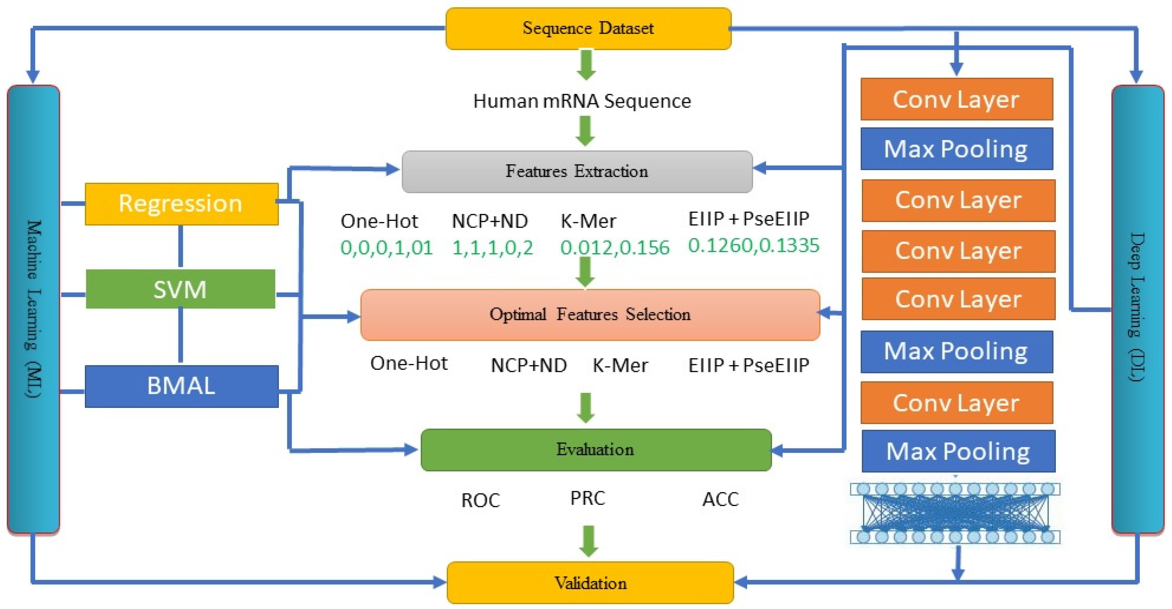
3. Materials and Methods

3.1. Regression

The goal of linear regression: Obtain a function f that satisfies f(a) = ˆb, where a ∈ R n, bˆ ∈ R, making bˆ close to the real label y, so the define output of linear regression as Equation (1).

$$f\left(a\right)=n^{T}a$$

(1)

where w ∈ R n is the parameter that needs to learn, in regression, task is definite by T: predict b from a and output is bˆ = n⊤a. It is defined P as performance metric and assume that the features and labels of test set are A(test) and B(test) and it can be used as mean square error (MSE). If bˆ^(test) represents the predicted value of the model on the test dataset, then the average error formula is defined as Equation (2).

$$MS{E}_{test}=\frac{1}{n}{\displaystyle \sum }{(b^{^\left(test\right)}-b^{\left(test\right)})}_i^2=||(b^{^\left(test\right)}-b^{\left(test\right)})|{|}_2^2$$

(2)

In order to build a machine learning algorithm, it is necessary to design an algorithm, by observing the training set (A(train), B(train)) and gain experience to improve the weight w to reduce MSE test. An intuitive way is, minimize the mean square error (MSE) on the training dataset, namely MSE train. To minimize mean square error train, we can simply solve the case, where the derivative is 0: define in Equation (3).

$$\begin{array}{c}{\nabla }_{w}MS{E}_{train}=0\\ \Rightarrow {\nabla }_w\frac{1}{m}\left|\right|\left(b^{^\left(train\right)}-b^{^\left(test\right)}\right)|{|}_2^2=0\\ \Rightarrow {\nabla }_w\frac{1}{m}|\left|\left(A^{\left(trian\right)}w-b^{\left(train\right)}\right)\right|{|}_2^2=0\\ \Rightarrow w={(A^{\left(trian\right)T}{A}^{\left(train\right)})}^{\left(-1\right)})A^{\left(train\right)\left(T\right)}{b}^{\left(train\right)}\\ {\nabla }_{w}MS{E}_{train}=0\\ \Rightarrow {\nabla }_w\end{array}$$

(3)

The solution of the program: w = (A^(train) ⊤ A^(train)) −1 A^(train) ⊤ B^(train) is called a regular course. The function f(a) = ca + d is called an affine function. When d = 0, it becomes f(a) = ca, which is called a linear function, and it is special case of an affine function.

3.2. SVM

It will put (A(i), B(i)) writing (Ai, Bi), write the j-th feature of sample a as aj. If the function interval.

Γˆ = 1, then γe =1/∥w∥. The above target function is transformed into it, Equation (4) represent this function.

$$\begin{array}{c}\{\max \frac{1}{\left|\left|w\right|\right|}\\ \{s.t.,y_i\left(w^T{A}_i+B\right)={\gamma }_i^\ge ,1.i=1\mathrm{I}.,n\end{array}$$

(4)

Equation (5) is equivalent to solving function.

$$\begin{array}{c}\left\{\min \frac{1}{2}\right|\left|w\right|{|}^2\\ \{s.t.,y_i\left(w^T{A}_i+b\right)={\gamma }_i^\ge ,1.iI....,n\end{array}$$

(5)

Identification ac4C problems can be solved naturally, introducing the kernel function and progressing to the non-linear classification problem. In Equation (6), define the Lagrangian function as follows.

$$\ell \left(w,B,\alpha \right)=\frac{1}{2}||w|{|}^2-{\displaystyle \sum }_{i=1}^n{\alpha }_i[w^T\mathrm{A}+b-1]$$

(6)

The identification ac4C problem is broken down into three steps: (1) Let L (w, b) be minimized in terms of w and b. (2) In the dual problem, use the SMO algorithm to solve the Lagrangian multiplication and find the extreme magnitude. (3) Determine the parameters w and b. First, fix and minimize L in relation to w and band. In Equation (7), find the partial derivatives of w and b.

$$\begin{array}{c}\{\frac{\partial l}{\partial w}=0\Rightarrow w={\displaystyle \sum _{i=1}^n}{a}_i{B}_i{A}_i\\ \{\frac{\partial l}{\partial B}=0\Rightarrow {\displaystyle \sum _{i=1}^n}{a}_i{B}_i=0\end{array}$$

(7)

Substitute the original formula to obtain Equations (8) and (9).

$$\begin{array}{c}\ell \left(W,B,\alpha \right)=\frac{1}{2}{w}^T.{\displaystyle \sum _{i=1}^n}{\alpha }_i{A}_i\mathrm{B}-w^T{\displaystyle \sum _{i=1}^n}{\alpha }_i{B}_i{A}_i\\ -b{\displaystyle \sum _{i=1}^n}{\alpha }_i{B}_i+{\displaystyle \sum _{i=1}^n}{a}_i\end{array}$$

(8)

$$\begin{array}{c}=-\frac{1}{2}{w}^T·{\displaystyle \sum _{i=1}^n}{\alpha }_i{B}_i{A}_i-b{\displaystyle \sum _{i=1}^n}{\alpha }_i{B}_i+{\displaystyle \sum _{i=1}^n}{\alpha }_i\\ =-\frac{1}{2}{\left[{\displaystyle \sum _{i=1}^n}{\alpha }_i{B}_i{A}_i\right]}^T{\displaystyle \sum _{i=1}^n}{\alpha }_i{B}_i{A}_i-b{\displaystyle \sum _{i=1}^n}{\alpha }_i{B}_i+{\displaystyle \sum _{i=1}^n}{\alpha }_i\\ =-\frac{1}{2}{\displaystyle \sum _{i=1}^n}{\alpha }_i{B}_i{\left(A_i\right)}^T·{\displaystyle \sum _{i=1}^n}{\alpha }_i{B}_i{A}_i-b{\displaystyle \sum _{i=1}^n}{\alpha }_{i}y{B}_i+{\displaystyle \sum _{i=1}^n}{\alpha }_i\\ =-\frac{1}{2}{\displaystyle \sum _{i,j=1}^n}{\alpha }_i{\alpha }_j{B}_i\mathrm{B}{A}_i^T{A}_j+{\displaystyle \sum _{i=1}^n}{\alpha }_i\end{array}$$

(9)

Using SMO algorithm to solve the identification ac4C in the dual problem, the target function is obtained, which is represented in Equations (10) and (11).

$$\begin{array}{c}{\max }_{\alpha }{\displaystyle \sum _{i=1}^n}{a}_i-{\displaystyle \sum _{i=1}^n}{\alpha }_i{\alpha }_j{B}_i\mathrm{B}{A}_i^T\mathrm{A}\\ s.t.,{\alpha }_i\ge 0I=1,....,n\end{array}$$

(10)

$${\displaystyle \sum }_{i=1}^n{a}_i{B}_i=0$$

(11)

The identification ac4C, α in the dual problem can be solved by the SMO algorithm. Find the parameters w, b, in the previous step, the Lagrange multiplied by α is obtained, and we can calculate: $w^{*}={{\displaystyle \sum }}_{i=1}^m{a}_{i }$ $B_{i }{A}_{i }$Because the support vector is at the boundary point, it satisfies Equations (12)–(18).

$$\begin{array}{c}\{{\max }_{B_i=-1}{w}^T{A}_i+b=-1\\ \{{\min }_{B_i=1}{w}^T{A}_i+b=1\end{array}$$

(12)

$$f\left(A\right)={\left({\displaystyle \sum }_{i=1}^n{a}_i{B}_i{A}_i\right)}^{T}A+b$$

(13)

$$={\displaystyle \sum }_{i=1}^n{a}_i{B}_i\langle A_i,A\rangle +b$$

(14)

$$f\left(A\right)={\displaystyle \sum }_{i=1}^n{a}_i{B}_i\langle A_i,A\rangle +b$$

(15)

Mapped to

$$f\left(A\right)={\displaystyle \sum }_{i=1}^n{a}_i{B}_i\langle \Phi \left(\mathrm{A}\right),\Phi \left(A\right)\rangle +b_0$$

(16)

$$\begin{array}{c}{\max }_{\alpha }{\displaystyle \sum _{i=1}^n}{a}_i-\frac{1}{2}{\displaystyle \sum _{i=1}^n}{\alpha }_i{\alpha }_j{B}_i{B}_j\langle \Phi \left(A_i\right),\Phi \left(A\right)\rangle \\ s.t.,{\alpha }_i\ge 0I,i=1,....,n\end{array}$$

(17)

$${\displaystyle \sum }_{i=1}^n{a}_i{B}_i=0$$

(18)

3.3. Bayesian MAML (BMAML)

Instead of ac4c solutions being learned [39], BMAML simply maintains and optimizes M solutions. Subject-specific rapid weight(s) are attempts to maximize screen data (i.e., hood) by probabilistic MAMLs. This probability was modeled by Yoon et al. [40], stein variation discontinuation (SVGD) and Liu and Wang (2016) [40].

To obtain M solutions, or equivalently, parameter settings ${\theta }^m$, identification ac4C $\mathrm{\Theta }={\left\{{\theta }^m\right\}}_{i=1}^M$. At iteration t, every ${\theta }_t\in \mathrm{\Theta }$ is updated as follows, in Equations (19)–(21).

$${\theta }_{t+1}={\theta }_t+\epsilon (\mathrm{\Phi }({\theta }_t))$$

(19)

$$\mathrm{\Phi }({\theta }_t)=\frac{1}{M}{\displaystyle \sum _{m=1}^M[k({\theta }_t^m,{\theta }_t){\nabla }_{{\theta }_t^m}\log p({\theta }_t^m)+{\nabla }_{{\theta }_t^m}k({\theta }_t^m,{\theta }_t)]}$$

(20)

$$p(y_j^{test}|{\theta }_j^{\prime })\approx \frac{1}{M}{\displaystyle \sum _{m=1}^{M}p(y_j^{test}|{\theta }_{T_j}^m)}$$

(21)

The proposed meta-loss is then given by Equation (22).

$$L_{BMAML}({\mathrm{\Theta }}_0)={\displaystyle {\sum }_{T_j\in B}{\displaystyle \sum _{m=1}^M\left|\right|{\theta }_{T_j}^{n.m}}}-{\theta }_{T_j}^{n+s,m}|{|}_2^2$$

(22)

3.4. DL-ac4C

There are numerous deep-learning architectures, with CNNs and recurring neural networks being the two most common. NLP (natural language processing) and computer vision are commonly used by RNNs and CNNs respectively. Recent CNN-based works have allowed for DNA sequence training rather than preliminary feature extraction. RNN connections can generate a directory graph in a sequence, allowing RNNs to extract features from DNA sequences in a novel and efficient way [52,53,54,55,56,57,58,59,60].

For CNN, by the convergent process and sharing of parameters in comparison with neural networks, the number of model parameters is considerably reduced. Collective layers also can create raw function sequences. The pattern of the convolutional layer scan’s narrative patterns is similar to the standard position weight matrices. The pooling layer can be used to summarize a maximum value that can help reduce the fitness of certain adjacent neurons to activate. Fully integrated layers are also used for the construction of final, unilineal combinations on top of all layers after the extraction, as shown in Figure 1 and Equation (23).

$$J(\theta )=\frac{1}{2m}{\displaystyle \sum _{i=1}^m(y^{\wedge (i)}-}{y}^{(i)}{)}^2$$

(23)

Gradient calculation: Take a single sample as an example, suppose the output unit yˆ = g(z), g is the activation function of the output unit, and z is the function of θ, then the cost function is 1/2(g(z) − y)2 can be calculated as the gradient: Equations (24) and (25).

$$\frac{\partial J(\theta )}{\partial z}=(g(z)-y)g^{\prime }(z)$$

(24)

$$\arg {\min }_{\theta }-L(\theta |y,y^{\wedge })$$

(25)

The likelihood L (θ|y, yˆ) can be expressed as a joint probability: Equation (26).

$$P(t,z|\theta )=P(t|z,\theta )P(z|\theta )$$

(26)

If the output unit is a sigmoid unit used in Bernoulli output distribution, the corresponding cost function can be obtained: Equation (27).

$$J(\theta )=ar{\min }_{\theta }-L(\theta |y,y^{\wedge })=-\frac{1}{m}{\displaystyle \sum _{i=1}^m(y^{(i)}\log y^{\wedge (i)}+(}1-y^{(i)})\log (1-y^{\wedge (i)}))$$

(27)

Gradient calculation: Taking a single sample as an example, suppose the output unit yˆ = g(z), g is the activation function of the output unit, and z is the function of θ. The gradient can be calculated: Equation (28).

$$\frac{\partial J(\theta )}{\partial z}=-(\frac{y}{g(z)}-\frac{(1-y)}{1-g(z)})g^{\prime }(z)$$

(28)

If g is a sigmoid function, it can be simplified further: in Equations (29)–(31).

$$J(\theta )=-yz+\log (1+e^z)$$

(29)

$$\frac{\partial J(\theta )}{\partial z}=\sigma (z)-y$$

(30)

$$J(\theta )=\arg {\min }_{\theta }-L(\theta |y,y^{\wedge })=-\frac{1}{m}{\displaystyle \sum _{i=1}^m{y}^{(i)}\log y^{\wedge (i)}})$$

(31)

where for each yˆ there is ${y^{\wedge }}_y=\frac{\exp (z_k)}{{\displaystyle {\sum }_j\exp (z_j)}}$ so it can be further expanded to Equation (32).

$$J(\theta )=-\frac{1}{m}{\displaystyle \sum _{i=1}^m{\displaystyle \sum _{k=0}^{K-1}(y_k^{(i)}\log y_k^{\wedge (i)})}}$$

(32)

Gradient calculation: Taking a single sample as an example, assuming that the output unit yˆ = g(z), g is the activation function of the output unit, then the cost function is:

$$J(\theta )=-{\displaystyle \sum _{k=0}^{K-1}{y}_k}\log y_k^{\wedge }$$

3.5. The ac4C Deep Learning Model (ac4C-DL)

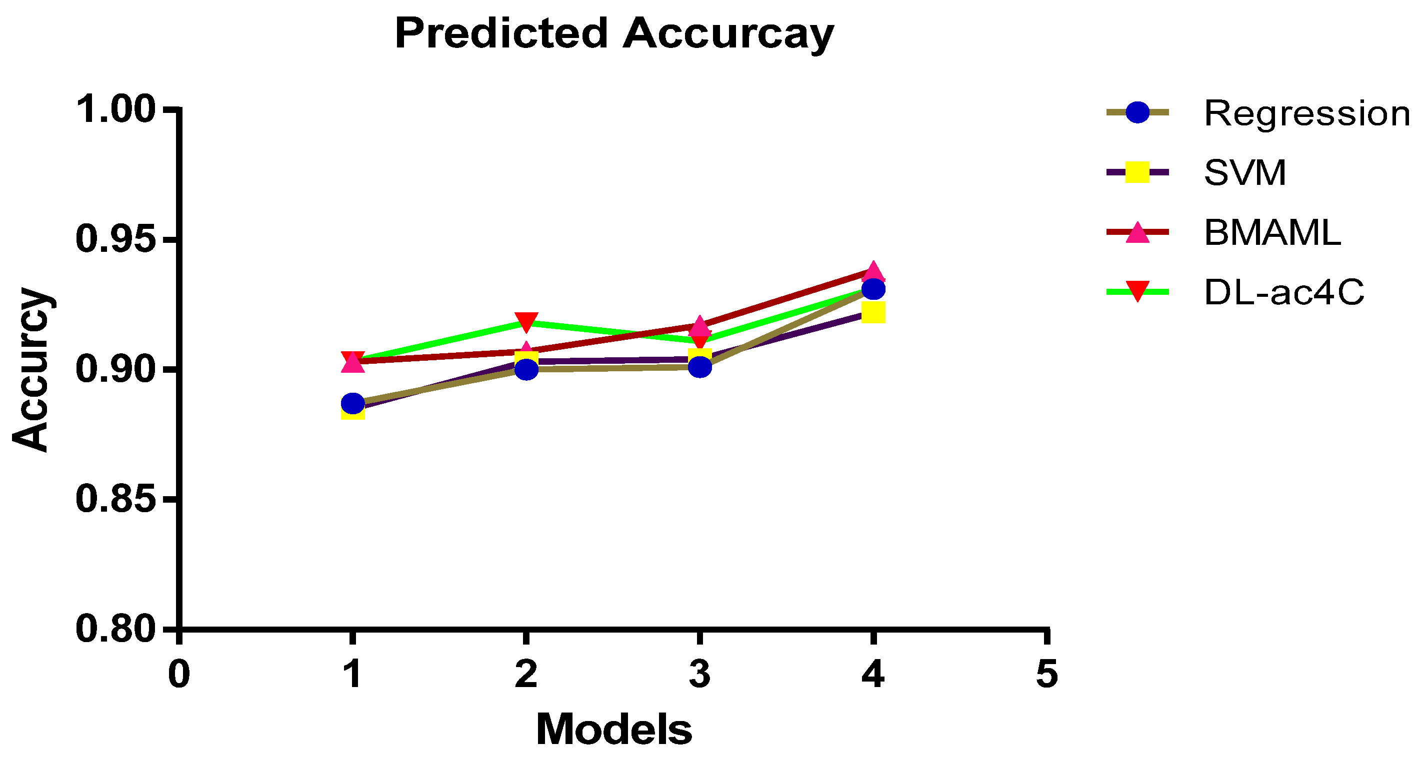
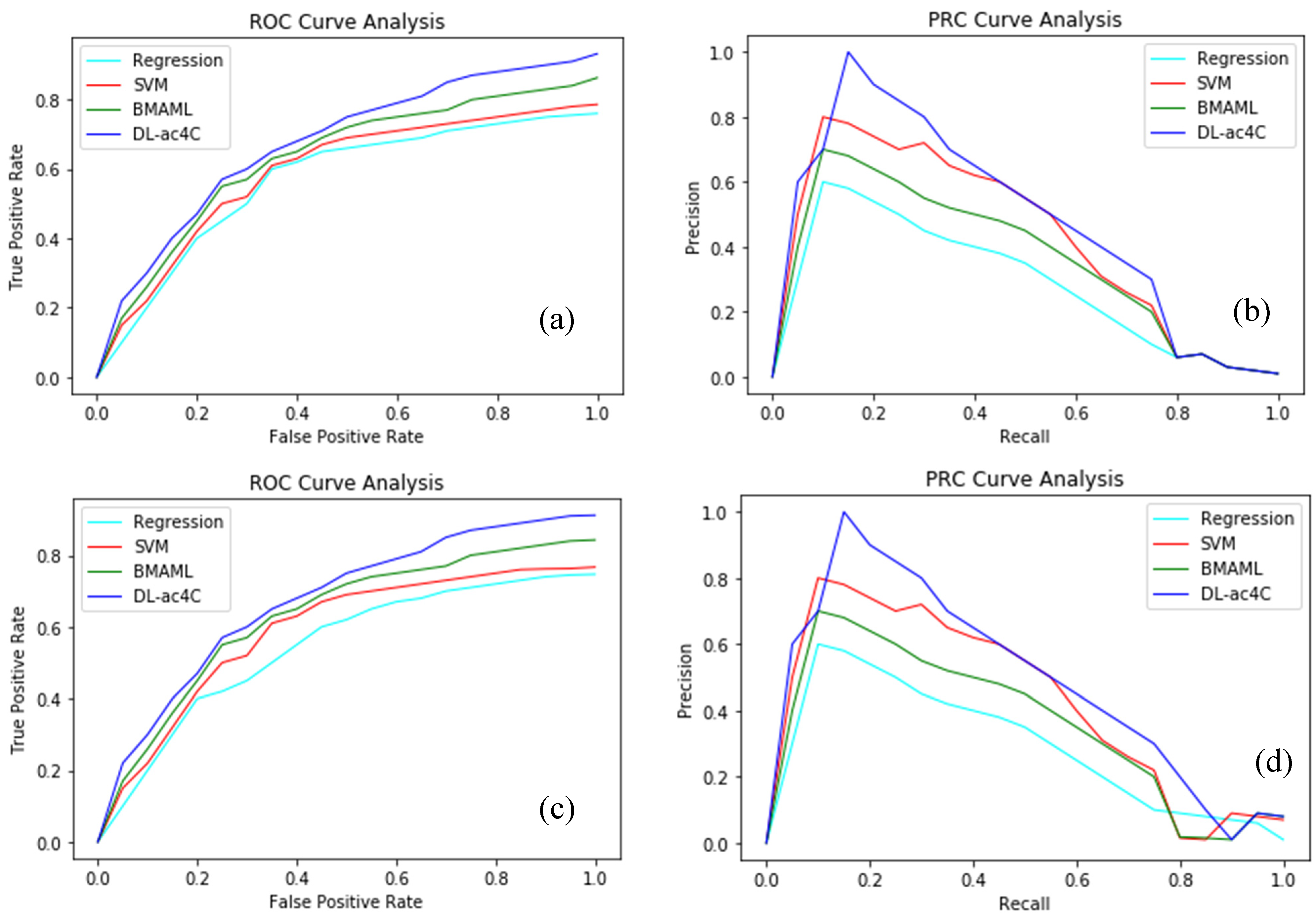
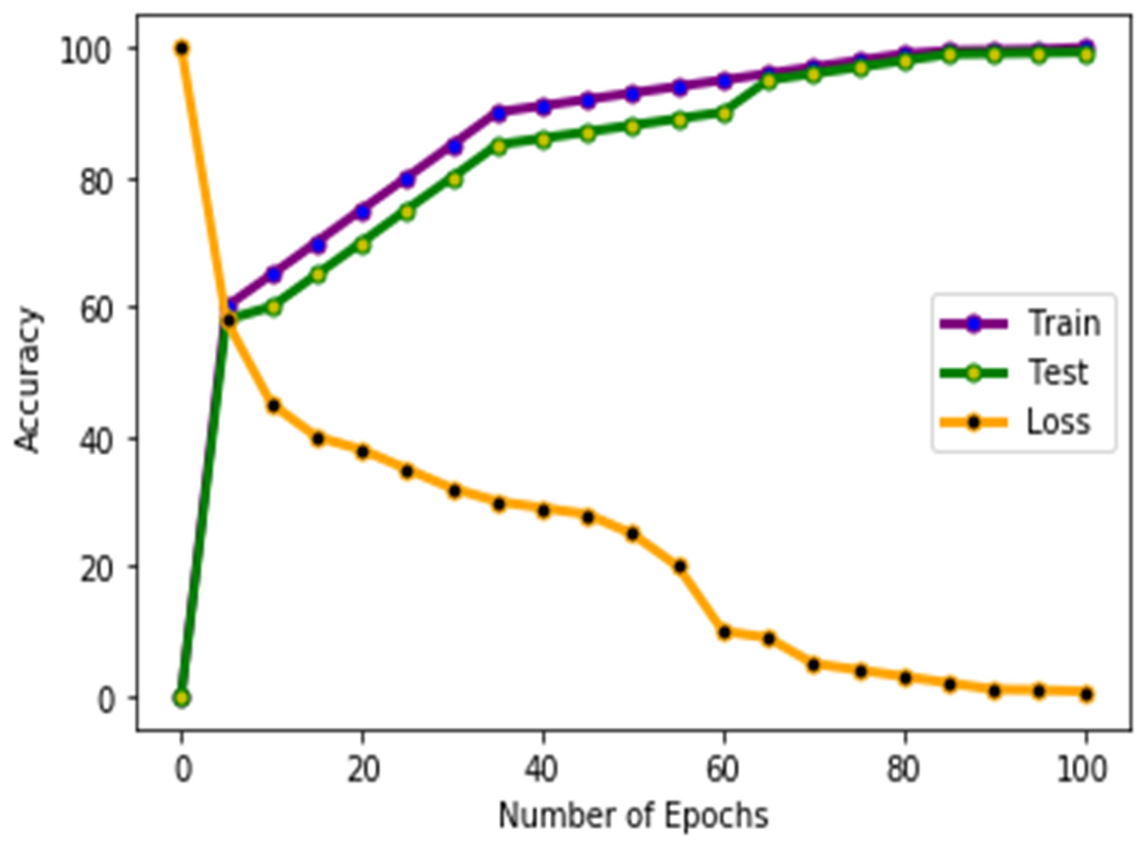
Several models were tested to determine which neural network predicted the best mRNA. Based on traditional architectural-deep learning, three types of models were built: CNN, RNN and hybrid combinations, Figure 2 shows the predicted accuracy of different models. Figure 3 shows the first conv layer (CL), max pooling (MP), second conv layer (SCL), third conv layer (TCL), fourth conv layer (FCL), max pooling (MP), fifth conv layer (FIFCL), max pooling (MP), and last layer is fully connected layer (FCL).

To address this issue, we developed a CNN neural model (DL-ac4C) and compared it to other models. CNNs are rarely employed in the construction of gene sequences. DanQ’s CNN-RNN architecture included the other four architectures (CMBLF, CCMBLF, CMBGF, and CCMBGF). We chose the model with the best predictive potential for the problem of mRNA prediction from the above-mentioned architectures. The proposed DL-ac4C model is depicted in Figure 1.

Recently, a PACES predictor for the classification of ac4C sites in human mRNA was proposed’. The PACES’ effects are still evolving, in this study, we propose a computer model that focuses on a deep learning approach to assessing mRNA DL-ac4C sites. Chemical properties of nuclearotide (CIP), nucleotide density (K-Mer), single-hot encoding, pseudopotennial EIIP, and pseudopotennial ion trinucleotide were among the benchmark datasets (PseEIIP). Various assessment metrics, all widely used in bio-informatically applications, namely precision, sensitivity, and specificity, were used to test DL-ac4C. We also focus on the recipient operational features (ROC) and the recall curve (PRC) due to unbalanced data sets. Thus, ROC and PRC performance are used to select the best representation vector characteristics and the optimum deeper learning classification. Figure 1 shows the proposed model DL-ac4C. We have developed various deep neural architectures to determine which deep neural architecture can produce good results, shown in

Table 1. The ac4C-DL model layer architecture and output layer dimension.

Numbers	Types	In_Put Size	Out_Put Size
1	INPUT LAYER	…	134 × 4
2	CONV LAYER	16 × 4 × 4	131 × 16
3	RELU LAYER	..	131 × 16
4	DROPOUT LAYER	..	131 × 16
5	CONV LAYER	16 × 4 × 4	128 × 64
6	RELU LAYER	..	128 × 64
7	POOL LAYER	4 × 2	64 × 64
8	BDLSTM LAYER	64 × 4 × 6	128 × 64
9	RELU LAYER	..	128 × 64
10	FULLY CONNECTED LAYER	128	128
11	DROPOUT LAYER	..	128 × 64
12	FULLY CONNECTED LAYER	One	One
13	SIGMOID LAYER	One	One

.

The column determines the size of the kernel, the maximum layer size of the window and the total layer size of the convolution layer.

4. Results

4.1. Experiments and Results

This article investigates data processing, libraries, and training model packages. The experimental setting and the computational efficiency of the proposed model are classical, simple, and in-depth learning models.

4.2. Data Source and Data Preprocessing

Benchmark and reference datasets were obtained from PACES (http://www.rnanut.net/paces/ accessed on 3 January 2022) in order to build a useful computational model. Datasets were collected from 2134 different chromosomes. The sites ac4C and non-ac4C of the negative and positive sequences were experimentally validated. There are five consecutive CXX patterns in each positive and negative sequence in the center where X {A, C, G, T} is located and the series span is 415 in the dataset. There are 1160 positive and 10,855 negative samples available for training. There are 469 positive and 4343 negative results in each test series. We used five-fold cross-validation for quality control purposes during the training phase. The training data set was five times divided into 232 positive and 2171 negative tests, respectively. The remaining fold was managed and four folds were used for preparation.

The extraction of functionality is critical in the development of efficient programming methods. To extract the characteristics of the mRNA sequences, the following 5 mRNA extraction methods were used in this study. DL-ac4C model’s training parameters are as follows: N estimator, 1200, study rate, 0.01, mini child weight, 5 maximum depths, 5 gammas 5, and 0.8.

One popular encoding is: RNA input sequence is encrypted using a single-hot technique, which gives A (1,0,0,0) encoding, C (0,1,0,0,0) encoding, G (0,0,1,0,0) encoding, and T (0,0,0,1) encoding (0,0,0,1). As a result, vector with a length of 415 = 4 = 1660 encoded each input sequence of the benchmark data set. The model employs a hot-end coding method, which is defined as the four-element binary per nucleotide to encode raw DNA or RNA sequences. The two vector types are as follows: a = [2, 0, 0, 0], C = [0, 1, 0, 0], G = [0, 0, 1, 0], and T = [0, 0, 0, 1]. The encoded bit matrix is then displayed as the DNA column sequence for A, C, G, and T. Binary vectors are DNA nucleotides that have only one input. We can keep the key position data for each nucleotide in the DNA sequences using a one-hot encoding technique, when we read each sequence, and it can notice a pattern. The size column displays kernel size, the pooling layer window size, and the overall layer size [61].

Nucleotide chemical property (NCP): the ring structure, feature groups, and hydrogen in the nucleotide mRNA chain can be divided into three groups, several recent studies have made use of a variety of chemical nucleotide properties. Amino A and G, Keto G and C, and Hydrogen A and T are all closely related, while hydrogen is only weakly related to C and G. A and G amino acid groups short, C and T are in one ring, while A and G are in two circles. Each mRNA sequence has a three-dimensional vector (x, y, z) that corresponds to the list of chemical characteristics in which x, y, z is drawn in Equations (33)–(35).

$$x_i=\{1,if,n_i\in \left\{A,C\right\}$$

(33)

$$=\{0,otherwise$$

$$y_i=\{1,if,n_i\in \left\{A,G\right\}$$

(34)

$$=\{0,otherwise$$

$$z_i=\{1,if,n_i\in \left\{A,T\right\}$$

(35)

$$=\{0,otherwise$$

In position x_i, y_i, and z_i are NCP nucleotide values, as a result, in each input sequence of the benchmark dataset, a vector with a length of 415 = 1245 was encoded. Nucleotide density (ND), the nucleotide density contains information about the automotive frequency and position in the mRNA sequence. The ND was used in several experiments. In Equations (36) and (37), the position j of ND di nucleotide n_j is indicated as:

$$d_i=\frac{1}{\left|N_i\right|}{\displaystyle \sum _{j=1}^{l}f(}{n}_j)$$

(36)

$$f(n_j)=\{1,if,n_j=p,p\in \left\{A,C,G,T\right\}$$

(37)

$$=\{0,otherwise$$

If Ni is the length of i-th prefix from the first position to i-th position, l is the length of the chain. For each input sequence, a 415-length vector was encoded in the benchmark datasets. Usually, we link the NCP to the ND. The resultant vector size is 1245 + 415 = 1660.

In this analysis, we used the K-mer form, K Mer, to define the mRNA sequence. K-mer refers to the approximate frequency of all potential k-sequences in longitude. Some problems have been addressed (23), (24). This item uses a single nucleotide (SN), a 2-mer di-nucleotide (DN) and a 3-nerve (DN). This article uses k = 1 and 2 and 3 (TN). Vectors with lengths of 4 + 16 + 64 = 84 have been coded for each input sequence of benchmark datasets.

PESEEIIP + EIP. The EIIP nucleotide values were suggested and used in bioinformatics to address various problems by the Nair and the Sreenadhan252. EIIP codes each nucleotide in the mRNA sequence to a numerical value that fits the free electron energy distribution. A has encoding of 0.1260, C has an encoding of 0.1340, G has 0.0806 and T 0.1335. Furthermore, PseEIIP is applied to MRNA sequence tri-nucleotides by taking the average EIIP value of each nucleotide. The 64-length PseEIIP vector encodes the mRNA sequence as follows in Equation (38).

$$PseEIIP=\left[EII{P}_{AAA}.f_{AAA},EII{P}_{AAC}.f_{AAC},.......EII{P}_{TTT}.f_{TTT}\right]$$

(38)

EIIPxyz = EIIPx + EIIPy + EIIPz, and x, y, z shall be true for {A, C, G, T} when Fxyz is the normalised frequency of I th Trinucleotide. The PseEIIP vector is 64 as a result. Therefore, a vector with a length of 415 + 64 = 479 has encoded every input of the benchmark data set. The Vector 415 represents the EIIP sequence values and the Vector 64 represents the PseEIIP value of the input sequence. The

Table 2. DL-ac4C and comparison with existing methods.

Classifier	Features	ROC	PRC	ACC
Regression	One-Hot	0.812	0.381	0.887
	NCP + ND	0.976	0.392	0.885
	K-mer	0.842	0.274	0.903
	EIIP + PseEIIP	0.780	0.354	0.903
SVM	One-Hot	0.784	0.361	0.900
	NCP+ND	0.821	0.384	0.903
	K-mer	0.847	0.429	0.907
	EIIP + PseEIIP	0.849	0.527	0.918
BMAML	One-Hot	0.787	0.364	0.901
	NCP+ND	0.799	0.348	0.904
	K-mer	0.847	0.502	0.917
	EIIP + PseEIIP	0.863	0.514	0.911
DL-ac4C	One-Hot	0.881	0.569	0.931
	NCP+ND	0.914	0.606	0.922
	K-mer	0.901	0.559	0.938
	EIIP + PseEIIP	0.932	0.663	0.931

shows the detail comparison between traditional machine learning (regression SVM and BMAML) and our proposed method (DL-acc4C), our method gives better accuracy, ROC and PRC. Figure 2 shows the predicted accuracy of different model. The dropout resulted in a nonlinear prediction line with an R2 score of 0.79.

4.3. Performance Metrics

The proposed model is evaluated in this study with the receiving operating curve region (ROC) and the recall area of precision (PRC). The PRC has the best choice to ‘test the model’s efficiency due to the imbalance of the benchmark data sets. Furthermore, in several recently published studies, accuracy (ACC), specificity (Sp) and sensitivity (Sn) have helped to evaluate the consistency of bioinformatics classification systems [52,54,55,56,57,61]. We are also using them to determine the model’s efficiency. If n+ represents acetylcytidine sties, then n− is represented at the non-acetylcytidine sites. It represented acetylcytidine sites that have been wrongly identified as non-acetylcytidine and is an incorrectly labelled number of non-acetylcytidine sites. These assessment measurements are described as in Equations (39)–(41). Figure 3 shows the comparison of different methods, on cross validation dataset and independent data test set. Figure 4 show the training process of DL-acc4C model and find very good accuracy and

Table 3. Comparison of deep learning DL-ac4C with existing models.

Dataset	Methods	ROC	PRC
Cross Validation	PACES	0.885	0.559
	XG-acc4C	0.91	0.653
	DL-acc4C	0.93	0.673
Independent	PACES	0.874	0.485
	XG-acc4C	0.889	0.581
	DL-acc4C	0.912	0.621

shows the detail comparison with existing methods (PACES and XG-acc4C) [61] and proposed method (DL-acc4C), on the bases of ROC and PRC and find better result from proposed method. Figure 3 shows the training process of DL-acc4C model.

$$ACC=1-(\frac{n_{-}^{+}+n_{+}^{-}}{n^{+}+n^{-}})$$

(39)

$$SN=1-(\frac{n_{-}^{+}}{n^{+}})$$

(40)

$$SN=1-(\frac{n_{+}^{-}}{n^{-}})$$

(41)

5. Discussions

The paper offers an initial estimate of the direct use in mRNA gene expression databases of current profound learning models. In particular, for two separate feature reduction methods (LASSO standard), a multi-layer art neural feedback network as a technical learning model was used as a basic test and performance model (corrected linear model). The study applied an honest validation approach to the evaluation of the three data sets of the public sequence. Both the reduction of characteristics and the models were tested by a train data set.

Generally speaking, the combination of deep learning models and the two considered reduction techniques rarely exceeds the basic AUC norm of LASSO. In addition, the estimation of the proposed deep-learning method, based on the number of parameters to be changed in these models, would require at least a five-fold delay of LASSO, implying that deep-learning is not proposed as an estimate ‘of the patient’s vital status from the RNA-Seq data under these conditions. Examining this research line leads to the conclusion that it will take us a long time to complete a simple feature-reduction technology to achieve comparable predictive efficiency and reduce gene quantity to match a deep-learning model.

Despite the lack of brilliant results in this work, no negative contact is important for the use of in-depth learning in RNA-Seq data analysis. On the contrary, there is a great deal of hope that this model will improve its predictive efficiency. In this respect, these works have made it possible for us to see that the smart use of deep learning models is essential for productivity in this field. For example, to compact information on 20,000 genes in fewer variables, deep learning can be used as an automatic stacked encoder that is used as inputs in any other compressed function of any other ML model. Contrasting deeper learning models, taking biological information into account, can lead to better performance. At the end, it would be desirable to find ways to view this model clinically. That is why it could be a plausible way for us to understand network architecture through an established knowledge of the relationship between individual nuclear polymorphisms, chromosomes, pathways, proteins, etc. The sequence validation confusion matrix is shown in Figure 5.

6. Conclusions

mRNA post-transcriptional modification is a component that plays an important role in mRNA stability control and translation. Identifying mRNA changes in laboratory experiments is difficult; therefore, we developed a new deep learning method for recognizing mRNA changes. We developed DL-ac4C, a CNN-based deep learning model for ac4C recognition, in this study. We used genomic sequence data, and after removing redundant data, mRNA genomic sequences were transferred to encoded bit matrices using the one-hot encoding method. By contrasting classification efficiency with simple deep learning methods across a variety of useful steps, our model was designed based on CNN, trained, and chosen with the highest evaluation results (ROC and PRC), competing with deep learning research models from architectures (DL-ac4C). This study developed a comprehensive and useful learning model for identifying acetylated mRNA sites. Using EIIP features, the proposed model predicts ac4C with high accuracy (0.931%). The DL-ac4C model outperforms some machine learning methods (regression, SVM, and BMAML), and for cross-validation and independence, our model DL-ac4C outperforms PACES and XG-acc4C. Ac4C has also been linked to a number of human diseases, the current ac4C in mRNA mechanism is based on human HeLa cells and needs to be refined in other species and cell types. As detection methods improve, the role of ac4C in disease diagnosis and prognosis will become clearer.

References

1. Yoon, J.; Kim, T.; Dia, O.; Kim, S.; Bengio, Y.; Ahn, S. Bayesian Model Agnostic Meta-Learning. In Proceedings of the 32nd International Conference on Neural Information Processing Systems, NIPS’18, Montreal, QC, Canada, 3–8 December 2018; pp. 7332–7342. [Google Scholar]
2. Liu, Q.; Wang, D. Stein Variational Gradient Descent: A General-Purpose Bayesian Inference Algorithm. In Proceedings of the 30th International Conference on Neural Information Processing Systems, NIPS’16, Barcelona, Spain, 5–10 December 2016; pp. 2378–2386. [Google Scholar]
3. Boccaletto, P.; Machnicka, M.A.; Purta, E.; Piątkowski, P.; Bagiński, B.; Wirecki, T.K.; Bujnicki, J.M. MODOMICS: A database of RNA modification pathways. Nucleic Acids Res. 2018, 46, D303–D307. [Google Scholar] [CrossRef] [PubMed]
4. Sharma, S.; Langhendries, J.L.; Watzinger, P.; Kötter, P.; Entian, K.D.; Lafontaine, D.L. Yeast kre33 and human nat10 are conserved 18s rrna cytosine acetyltransferases that modify trnas assisted by the adaptor tan1/thumpd1. Nucleic Acids Res. 2015, 43, 2242–2258. [Google Scholar] [CrossRef] [PubMed] [Green Version]
5. Arango, D.; Sturgill, D.; Alhusaini, N.; Dillman, A.A.; Sweet, T.J.; Hanson, G.; Hosogane, M.; Sinclair, W.R.; Nanan, K.K.; Mandler, M.D.; et al. Acetylation of cytidine in mrna promotes translation efciency. Cell 2018, 175, 1872–1886. [Google Scholar] [CrossRef] [Green Version]
6. Zhao, W.; Zhou, Y.; Cui, Q.; Zhou, Y. PACES: Prediction of N4-acetylcytidine (ac4C) modification sites in mRNA. Sci. Rep. 2019, 9, 11112. [Google Scholar] [CrossRef] [Green Version]
7. Tahir, M.; Hayat, M. iNuc-STNC: A sequence-based predictor for identification of nucleosome positioning in genomes by extending the concept of SAAC and Chou’s PseAAC. Mol. BioSyst. 2016, 12, 2587–2593. [Google Scholar] [CrossRef]
8. Hayat, M.; Tahir, M. Psdentification: Identifcation of transmembrane helix segments using ensemble feature space by incorporated fuzzy support vector machine. Mol. BioSyst. 2015, 11, 2255–2262. [Google Scholar] [CrossRef] [PubMed]
9. Tahir, M.; Hayat, M.; Chong, K.T. Prediction of n6-methyladenosine sites using convolution neural network model based on distributed feature representations. Neural Netw. 2020, 129, 385–391. [Google Scholar] [CrossRef] [PubMed]
10. Tayara, H.; Oubounyt, M.; Chong, K.T. Identifcation of promoters and their strength using deep learning. IBRO Rep. 2019, 6, S552–S553. [Google Scholar] [CrossRef]
11. Tahir, M.; Hayat, M.; Ullah, I.; Chong, K.T. A deep learning-based computational approach for discrimination of dna n6-methyladenosine sites by fusing heterogeneous features. Chemomet. Intell. Lab. Syst. 2020, 206, 104151. [Google Scholar] [CrossRef]
12. Chicco, D. Ten Quick tips for machine learning in computational biology. BioData Mining 2017, 10, 35. [Google Scholar] [CrossRef]
13. Alam, W.; Tayara, H.; Chong, K.T. i4mC-Deep: An Intelligent Predictor of N4-Methylcytosine Sites Using a Deep Learning Approach with Chemical Properties. Genes 2021, 12, 1117. [Google Scholar] [CrossRef] [PubMed]
14. Manyika, J.; Chui, M.; Brown, B.; Bughin, J.; Dobbs, R.; Roxburgh, C.; Hung Byers, A. Big Data: The Next Frontier for Innovation, Competition, and Productivity; McKinsey Global Institute: Washington, DC, USA, 2011. [Google Scholar]
15. Ferrucci, D.; Brown, E.; Chu-Carroll, J.; Fan, J.; Gondek, D.; Kalyanpur, A.A.; Lally, A.; Murdock, J.W.; Nyberg, E.; Prager, J.; et al. Building Watson: An overview of the DeepQA project. AI Mag. 2010, 31, 59–79. [Google Scholar] [CrossRef] [Green Version]
16. IBM and Oncology. Available online: https://www.ibm.com/watson-health/solutions/cancer-research-treatment (accessed on 3 January 2022).
17. Silver, D.; Huang, A.; Maddison, C.J.; Guez, A.; Sifre, L.; Van Den Driessche, G.; Schrittwieser, J.; Antonoglou, I.; Panneershelvam, V.; Lanctot, M.; et al. Mastering the game of Go with deep neural networks and tree search. Nature 2016, 529, 484–489. [Google Scholar] [CrossRef] [PubMed]
18. Powles, J.; Hodson, H. Google DeepMind and healthcare in an age of algorithms. Health Technol. 2017, 7, 351–367. [Google Scholar] [CrossRef] [PubMed] [Green Version]
19. Iqbal, M.S.; Ahmad, I.; Bin, L.; Khan, S.; Rodrigues, J.J. Deep learning recognition of diseased and normal cell representation. Trans. Emerg. Telecommun. Technol. 2020, 32, e4017. [Google Scholar] [CrossRef]
20. Iqbal, M.S.; Luo, B.; Mehmood, R.; Alrige, M.A.; Alharbey, R. Mitochondrial Organelle Movement Classification (Fission and Fusion) via Convolutional Neural Network Approach. IEEE Access 2019, 7, 86570–86577. [Google Scholar] [CrossRef]
21. Iqbal, M.S.; Khan, T.; Hussain, S.; Mahmood, R.; El-Ashram, S.; Abbasi, R.; Luo, B. Cell Recognition of Microscopy Images of TPEF (Two Photon Excited Florescence) Probes. Procedia Comput. Sci. 2019, 147, 77–83. [Google Scholar] [CrossRef]
22. Iqbal, M.S.; El-Ashram, S.; Hussain, S.; Khan, T.; Huang, S.; Mehmood, R.; Luo, B. Efficient cell classification of mitochondrial images by using deep learning. J. Opt. 2019, 48, 113–122. [Google Scholar] [CrossRef]
23. Larrañaga, P.; Calvo, B.; Santana, R.; Bielza, C.; Galdiano, J.; Inza, I.; Lozano, J.A.; Armananzas, R.; Santafé, G.; Pérez, A.; et al. Machine learning in bioinformatics. Brief. Bioinform. 2006, 7, 86–112. [Google Scholar] [CrossRef] [PubMed] [Green Version]
24. LeCun, Y.; Bengio, Y.; Hinton, G. Deep learning. Nature 2015, 521, 436–444. [Google Scholar] [CrossRef]
25. Jones, D.T. Protein secondary structure prediction based on position-specific scoring matrices. J. Mol. Biol. 1999, 292, 195–202. [Google Scholar] [CrossRef] [Green Version]
26. Ponomarenko, J.V.; Ponomarenko, M.P.; Frolov, A.S.; Vorobyev, D.G.; Overton, G.C.; Kolchanov, N.A. Conformational and physicochemical DNA features specific for transcription factor binding sites. Bioinformatics 1999, 15, 654–668. [Google Scholar] [CrossRef] [PubMed]
27. Cai, Y.-D.; Lin, S.L. Support vector machines for predicting rRNA-, RNA-, and DNA-binding proteins from amino acid sequence. Biochim. Biophys. Acta BBA-Proteins Proteom. 2003, 1648, 127–133. [Google Scholar] [CrossRef]
28. Atchley, W.R.; Zhao, J.; Fernandes, A.D.; Drüke, T. Solving the protein sequence metric problem. Proc. Natl. Acad. Sci. USA 2005, 102, 6395–6400. [Google Scholar] [CrossRef] [PubMed] [Green Version]
29. Branden, C.I. Introduction to Protein Structure; Garland Science: New York, NY, USA, 1999. [Google Scholar]
30. Richardson, J.S. The anatomy and taxonomy of protein structure. Adv. Protein Chem. 1981, 34, 167–339. [Google Scholar]
31. Lyons, J.; Dehzangi, A.; Heffernan, R.; Sharma, A.; Paliwal, K.; Sattar, A.; Zhou, Y.; Yang, Y. Predicting backbone Cα angles and dihedrals from protein sequences by stacked sparse auto-encoder deep neural network. J. Comput. Chem. 2014, 35, 2040–2046. [Google Scholar] [CrossRef] [PubMed] [Green Version]
32. Heffernan, R.; Paliwal, K.; Lyons, J.; Dehzangi, A.; Sharma, A.; Wang, J.; Sattar, A.; Yang, Y.; Zhou, Y. Improving prediction of secondary structure, local backbone angles, and solvent accessible surface area of proteins by iterative deep learning. Sci. Rep. 2015, 5, 11476. [Google Scholar] [CrossRef] [Green Version]
33. Spencer, M.; Eickholt, J.; Cheng, J. A Deep Learning Network Approach to ab initio Protein Secondary Structure Prediction. Computational Biology and Bioinformatics. IEEE/ACM Trans. Comput. Biol. Bioinform. 2015, 12, 103–112. [Google Scholar] [CrossRef] [Green Version]
34. Nguyen, S.P.; Shang, Y.; Xu, D. DL-PRO: A novel deep learning method for protein model quality assessment. In Proceedings of the 2014 International Joint Conference on Neural Networks (IJCNN), Beijing, China, 6–11 July 2014; pp. 2071–2078. [Google Scholar]
35. Baldi, P.; Brunak, S.; Frasconi, P.; Soda, G.; Pollastri, G. Exploiting the past and the future in protein secondary structure prediction. Bioinformatics 1999, 15, 937–946. [Google Scholar] [CrossRef] [PubMed] [Green Version]
36. Baldi, P.; Pollastri, G.; Andersen, C.A.; Brunak, S. Matching protein beta-sheet partners by feedforward and recurrent neural networks. In Proceedings of the 2000 Conference on Intelligent Systems for Molecular Biology (ISMB00), La Jolla, CA, USA, 19–23 August 2000; pp. 25–36. [Google Scholar]
37. Sønderby, S.K.; Winther, O. Protein Secondary Structure Prediction with Long Short-Term Memory Networks. arXiv 2014, arXiv:1412.7828 2014. [Google Scholar]
38. Lena, P.D.; Nagata, K.; Baldi, P.F. Deep spatio-temporal architectures and learning for protein structure prediction. In Advances in Neural Information Processing Systems; Massachusetts Institute of Technology Press: Cambridge, MA, USA, 2012; pp. 512–520. [Google Scholar]
39. Lena, P.D.; Nagata, K.; Baldi, P. Deep architectures for protein contact map prediction. Bioinformatics 2012, 28, 2449–2457. [Google Scholar] [CrossRef] [Green Version]
40. Baldi, P.; Pollastri, G. The principled design of large-scale recursive neural networ—Architectures—Dag-rnns and the protein structure prediction problem. J. Mach. Learn. Res. 2003, 4, 575–602. [Google Scholar]
41. Leung, M.K.; Xiong, H.Y.; Lee, L.J.; Frey, B.J. Deep learning of the tissue-regulated splicing code. Bioinformatics 2014, 30, i121–i129. [Google Scholar] [CrossRef] [Green Version]
42. Lee, T.; Yoon, S. Boosted Categorical Restricted Boltzmann Machine for Computational Prediction of Splice Junctions. In Proceedings of the 32nd International Conference on Machine Learning, Lille, France, 7–9 July 2015; pp. 2483–2492. [Google Scholar]
43. Zhang, S.; Zhou, J.; Hu, H.; Gong, H.; Chen, L.; Cheng, C.; Zeng, J. A deep learning framework for modeling structural features of RNA-binding protein targets. Nucleic Acids Res. 2015, 44, e32. [Google Scholar] [CrossRef] [PubMed] [Green Version]
44. Chen, Y.; Li, Y.; Narayan, R.; Subramanian, A.; Xie, X. Gene expression inference with deep learning. Bioinformatics 2016, 32, 1832–1839. [Google Scholar] [CrossRef] [Green Version]
45. Denas, O.; Taylor, J. Deep modeling of gene expression regulation in an Erythropoiesis model. In Proceedings of the International Conference on Machine Learning workshop on Representation Learning, Atlanta, GA, USA, 2–4 May 2013. [Google Scholar]
46. Alipanahi, B.; Delong, A.; Weirauch, M.T.; Frey, B.J. Predicting the sequence specificities of DNAand RNA-binding proteins by deep learning. Nat. Biotechnol. 2015, 33, 831–838. [Google Scholar] [CrossRef]
47. Zhou, J.; Troyanskaya, O.G. Predicting effects of noncoding variants with deep learning-based sequence model. Nat. Methods 2015, 12, 931–934. [Google Scholar] [CrossRef] [Green Version]
48. Lee, B.; Lee, T.; Na, B.; Yoon, S. DNA-Level Splice Junction Prediction using Deep Recurrent Neural Networks. arXiv 2015, arXiv:1512.05135. [Google Scholar]
49. Hochreiter, S.; Heusel, M.; Obermayer, K. Fast model-based protein homology detection without alignment. Bioinformatics 2007, 23, 1728–1736. [Google Scholar] [CrossRef] [PubMed] [Green Version]
50. Sønderby, S.K.; Sønderby, C.K.; Nielsen, H.; Winther, O. Convolutional LSTM Networks for Subcellular Localization of Proteins. arXiv 2015, arXiv:1503.01919. [Google Scholar]
51. Fakoor, R.; Ladhak, F.; Nazi, A.; Huber, M. Using deep learning to enhance cancer diagnosis and classification. In Proceedings of the International Conference on Machine Learning, Washington, DC, USA, 4–7 December 2013. [Google Scholar]
52. Do, D.T.; Le, T.Q.T.; Le, N.Q.K. Using deep neural networks and biological subwords to detect protein S-sulfenylation sites. Brief. Bioinform. 2021, 22, bbaa128. [Google Scholar] [CrossRef]
53. Tng, S.S.; Le, N.Q.K.; Yeh, H.Y.; Chua, M.C.H. Improved Prediction Model of Protein Lysine Crotonylation Sites Using Bidirectional Recurrent Neural Networks. J. Proteome Res. 2021, 21, 265–273. [Google Scholar] [CrossRef]
54. Bin Heyat, M.B.; Akhtar, F.; Khan, M.H.; Ullah, N.; Gul, I.; Khan, H.; Lai, D. Detection, Treatment Planning, and Genetic Predisposition of Bruxism: A Systematic Mapping Process and Network Visualization Technique. CNS Neurol. Disord.-Drug Targets 2020, 20, 755–775. [Google Scholar] [CrossRef] [PubMed]
55. Bin Heyat, M.B.; Lai, D.; Khan, F.I.; Zhang, Y. Sleep Bruxism Detection Using Decision Tree Method by the Combination of C4-P4 and C4-A1 Channels of Scalp EEG. IEEE Access 2019, 7, 102542–102553. [Google Scholar] [CrossRef]
56. Bin Heyat, M.B.; Akhtar, F.; Khan, A.; Noor, A.; Benjdira, B.; Qamar, Y.; Abbas, S.J.; Lai, D. A Novel Hybrid Machine Learning Classification for the Detection of Bruxism Patients Using Physiological Signals. Appl. Sci. 2020, 10, 7410. [Google Scholar] [CrossRef]
57. Khan, H.; Bin Heyat, M.B.; Lai, D.; Akhtar, F.; Ansari, M.A.; Khan, A.; Alkahtani, F. Progress in Detection of Insomnia Sleep Disorder: A Comprehensive Review. Current Drug Targets 2021, 22, 672–684. [Google Scholar] [CrossRef]
58. Abbasi, R.; Xu, L.; Wang, Z.; Chughtai, G.R.; Amin, F.; Luo, B. Dynamic weighted histogram equalization for contrast enhancement using for Cancer Progression Detection in medical imaging. In Proceedings of the 2018 International Conference on Signal Processing and Machine Learning, Shanghai, China, 28–30 November 2018; pp. 93–98. [Google Scholar]
59. Abbasi, R.; Chen, J.; Al-Otaibi, Y.; Rehman, A.; Abbas, A.; Cui, W. RDH-based dynamic weighted histogram equalization using for secure transmission and cancer prediction. Multimed. Syst. 2021, 27, 177–189. [Google Scholar] [CrossRef]
60. Khan, A.R.; Khan, S.; Harouni, M.; Abbasi, R.; Iqbal, S.; Mehmood, Z. Brain tumor segmentation using K-means clustering and deep learning with synthetic data augmentation for classification. Microsc. Res. Technol. 2021, 84, 1389–1399. [Google Scholar] [CrossRef]
61. Alam, W.; Tayara, H.; Chong, K.T. XG-ac4C: Identification of N4-acetylcytidine (ac4C) in mRNA using eXtreme gradient boosting with electron-ion interaction pseudopotentials. Sci. Rep. 2020, 10, 20942. [Google Scholar] [CrossRef]
Figure 1. The chosen deep learning model (DL-ac4C) with the best performance on the validation set, mRNA.
Applsci 12 01344 g001
Figure 2. Predicted accuracy of models.
Applsci 12 01344 g002
Figure 3. Graph (a) for cross validation test ROC, and graph (b) for cross validation test of PCR and graph (c) for independent test for ROC and graph (d) independent test of PRC.
Applsci 12 01344 g003
Figure 4. The training, test and loss of the DL-ac4C.
Applsci 12 01344 g004
Figure 5. Our proposed method, confusion matrix of cross and independent dataset, (a) Cross validation DL-acc4C and (b) independent validation DL-acc4C.
Applsci 12 01344 g005