Evaluation and Testing System for Automotive LiDAR Sensors

Abstract

The world is facing a great technological transformation towards fully autonomous vehicles, where optimists predict that by 2030 autonomous vehicles will be sufficiently reliable, affordable, and common to displace most human driving. To cope with these trends, reliable perception systems must enable vehicles to hear and see all their surroundings, with light detection and ranging (LiDAR) sensors being a key instrument for recreating a 3D visualization of the world in real time. However, perception systems must rely on accurate measurements of the environment. Thus, these intelligent sensors must be calibrated and benchmarked before being placed on the market or assembled in a car. This article presents an Evaluation and Testing Platform for Automotive LiDAR sensors, with the main goal of testing both commercially available sensors and new sensor prototypes currently under development in Bosch Car Multimedia Portugal. The testing system can benchmark any LiDAR sensor under different conditions, recreating the expected driving environment in which such devices normally operate. To characterize and validate the sensor under test, the platform evaluates several parameters, such as the field of view (FoV), angular resolution, sensor’s range, etc., based only on the point cloud output. This project is the result of a partnership between the University of Minho and Bosch Car Multimedia Portugal.

1. Introduction

The world is undergoing an unprecedented technological transformation in which vehicles and autonomous driving systems are evolving at a breathtaking pace [1,2,3,4]. Optimistic predictions claim that by 2030 autonomous vehicles will be sufficiently reliable, affordable, and common to displace most human driving, providing huge savings and benefits [5]. However, most of the vehicles today are manually controlled, and in order to achieve full driving autonomy they must evolve through different levels of driving automation, as defined by the American Society of Automotive Engineers (SAE) [6]; levels 0—No Driving Automation, 1—Driver Assistance, and 2—Partial Driving Automation require a human driver to monitor the driving environment, while in levels 3—Conditional Automation, 4—High Automation, and 5—Full Automation the automated system is able to autonomously monitor and navigate the driving environment.

Current Level 2 vehicles are provided with advanced driver-assistance systems (ADAS) to help the driver in several situations, such as assisting in parking tasks, providing traffic alerts, promoting collision avoidance with other vehicles and objects, and performing automated decisions in situations that may compromise the safety of all occupants. Nonetheless, in order to cope with these revolutionary trends new solutions at the sensor level must be created to provide vehicles with the ability to hear and see the surrounding environment. An autonomous vehicle requires reliable sensors in order to recreate an accurate mapping of the surroundings, which is only possible with multi-sensor perception systems relying on a combination of radars, cameras, and light detection and ranging (LiDAR) sensors [7,8,9,10], as illustrated in Figure 1. Radar sensors can provide (1) cross-traffic alerts and Blind Spot Assist features, as well as assisting with (2) Adaptive Cruise Control systems; on the other hand, LiDAR sensors can be used to (3) translate the surroundings into a 3D representation, achieving several distances with high levels of accuracy and precision; finally, cameras can help with such features as (4) object detection and classification and (5) collision avoidance.

LiDAR sensors are emerging as a mandatory state-of-the-art technology that must be part of any perception system, as they enable a true 3D visualization of the surroundings through a point cloud representation in real time [11,12,13,14]. Accurate and precise measurement of the surroundings with LiDAR sensors can assist the perception systems in several tasks [9], e.g., obstacles, objects, and vehicles detection [15,16,17]; pedestrians recognition and tracking [18,19]; and ground segmentation for road filtering [20], among others [21]. Continual advances around LiDAR are improving its measuring and imaging architectures [12,22,23]. Nonetheless, the measurements and the 3D point cloud of a LiDAR sensor can always be corrupted by several noise sources, e.g., internal components [24], mutual interference [25,26], reflectivity issues [27], light [11], adverse weather conditions [10,28,29,30], and others [31], making it compulsory to test and analyze all sensors’ characteristics before they are placed on the market or assembled in a car. The first steps towards creating controlled environments for testing and evaluation of LiDAR sensors have already been taken. For instance, LIBRE [32], the first benchmarking and reference LiDAR dataset, tested ten sensors in three different environments and configurations: (1) static targets, where objects were placed at known distances and measured from a fixed position within a controlled environment; (2) adverse weather, where static obstacles were measured from a moving vehicle (captured in a weather chamber where LiDARs were exposed to different adverse conditions, such as fog, rain, and strong light); and (3) dynamic traffic, where dynamic objects were captured from a vehicle driven on public urban roads at multiple times and at different times of the day. These tests, further improved upon in [33], contributed to the evaluation of important parameters that play a crucial role on real-world LiDAR applications.

This article presents an evaluation and testing platform for automotive LiDAR sensors, designed to test commercially available sensors and sensor prototypes that are under development in Bosch Car Multimedia Portugal, S.A., before they are assembled for their final destination. The main goal of the testing platform is to rapidly test and validate sensors by analyzing only the point cloud output in order to validating the parameters previously tested and calibrated during the manufacturing phase. The testing system is able to benchmark any LiDAR sensor under real situations created in a controlled environment to recreate the expected driving conditions to which such devices are normally subjected. These conditions can be related to disturbances caused by different targets with different materials, compositions, reflectiveness, geometry, environmental factors, and noise conditions, among others. In order to characterize and validate the sensor under test, the testing platform evaluates several parameters, such as the field of view (FoV), angular resolution, sensor’ range, etc. The output of the evaluation and testing platform can be used to validate the sensor parameters under test and to assist in calibration of the perception system of the car. This article contributes to the state of the art with:

• An evaluation and testing platform for testing several parameters of a LiDAR sensor for automotive applications;
• A point cloud filter-based approach to evaluate several characteristics of a LiDAR sensor at the reception level;
• A desktop and an embedded approach for deploying the testing platform;
• Validation of the platform through testing and evaluation of a commercial off-the-shelf (COTS) LiDAR sensor.

2. LiDAR Sensors for Automotive

As a high-level overview, a LiDAR system is composed of two main components: an emitter (laser) and a receiver (light detector), as depicted in Figure 2. The laser emits short pulses of light with a well-defined time interval (a few to several hundred nanoseconds) and with specific spectral properties into the optical steering system. By regulating the mirror’s angle, the system controls the direction of the light vertically and horizontally, providing multiple angle detection with just a single beam. Additionally, the optical properties of the beam can be changed by the lens system in order to achieve better performance ratios, e.g., by adding signal modulation schemes [23,34]. When the transmitted light hits an object, the backscattered signal is collected by the receiver, which can filter and select specific wavelengths or polarization schemes. In addition, the receiver system is responsible for converting the optical signal into an electrical representation and storing it along with its intensity values in a computing unit. Moreover, the receiver calculates the time of travel of the transmitted light to obtain the distance to the obstacle. Within an automotive application, the main characteristics of a LiDAR sensor that need to be considered for inclusion in a LiDAR testing and evaluation platform are: (1) the horizontal and vertical field of view (FoV); (2) the horizontal and vertical angular resolution (AR); (3) the influence of external illumination; (4) power consumption; and (5) the sensor’s minimum and maximum ranges.

The aforementioned parameters are described in detail below:

• The Field of View is one of the metrics that defines the maximum angle at which a LiDAR sensor is able to detect objects, as shown in Figure 3. When two scanning angles are available, the sensor can scan a 3D area defined by the Vertical FoV (VFoV) and the Horizontal FoV (HFoV). This test is designed to identify the maximum detection angles of the sensor in order to validate its defined values.
• The Angular Resolution represents the sensor’s ability to scan and detect objects within the FoV, as depicted in Figure 4. Higher resolutions allow for smaller blind spots between laser firings, enabling the detection of small objects and greater detail of the environment, particularly at higher detection ranges. Thus, this test is designed to identify the angular resolution both vertically and horizontally in different areas of the FoV in order to verifying that the collected values match the requirements and/or the sensor’s characteristics as defined by the manufacturer.
• Background Light and Sunlight can have a severe impact on sensor behaviour. In real-world environments, LiDAR sensors may experience substantially decreased performance when exposed to external light interference, such as sunlight backscattering from targets with high reflectivity characteristics. Removing such light noise can be particularly challenging, as solar radiation is a powerful light source present in a wide range of wavelengths [35]. Therefore, it is important to evaluate sensor output when exposed to background light in a controlled environment.
• The Power Consumption test aims to monitor and analyze the power consumption of the sensor under test in different operation modes, configured parameters, and environment/target conditions.
• The Range can be defined as the minimum and the maximum distances at which the sensor successfully detects an object. While detecting the minimum range can be quite simple, finding the maximum range is not straightforward, and depends on the target’s reflectivity, which is considered detected when it appears in at least 90% (detection probability) of the the sensor’s data output. With a target reflectivity higher than 40–50%, detecting the maximum range in a straight line inside our testing laboratory (maximum range 100 m) would be impossible for high-range sensors. However, a sensor’s maximum range can be deduced from measurements performed on lower reflectivity targets by using the relationship between the returning signal strength from a specific target with a known reflectivity and its distance to the sensor. This method is based on the signal power arriving at the LiDAR detector as defined by the Equation (1), where A is a constant, $R_{lab}$ is the target’s reflectivity, and $r_{lab}^2$ is the target’s distance.

  $$P_{sig}={\displaystyle \frac{A{R}_{lab}}{r_{lab}^2}}$$

  (1)
  If the required minimum level for the returning signal remains the same regardless of the target’s reflectivity, the maximum distance can be calculated for any reflectivity value using Equation (2), where $R_{sim}$ is the target reflectivity to be simulated and $r_{sim}$ is the corresponding target distance calculated for the new reflectivity level. In order to reduce errors in the estimations, several measurements for the maximum range must be performed, e.g., targets with reflectivity of 10%, 20%, and 40%.

  $$r_{sim}=\sqrt{{\displaystyle \frac{R_{sim}{r}_{lab}^2}{R_{lab}}}}$$

  (2)

3. LiDAR Evaluation and Testing

The Evaluation and Testing Platform for Automotive LiDAR Sensors aims at the design and development of a test bench for LiDAR sensors (commercially available and Bosch prototypes currently under development) that is able to characterize and test the main parameters previously described in Section 2. Such tests are being performed at two Bosch locations: (1) the Optical Lab (range up to 23 m) and (2) the Long Range Measurements lab (range up to 100 m).

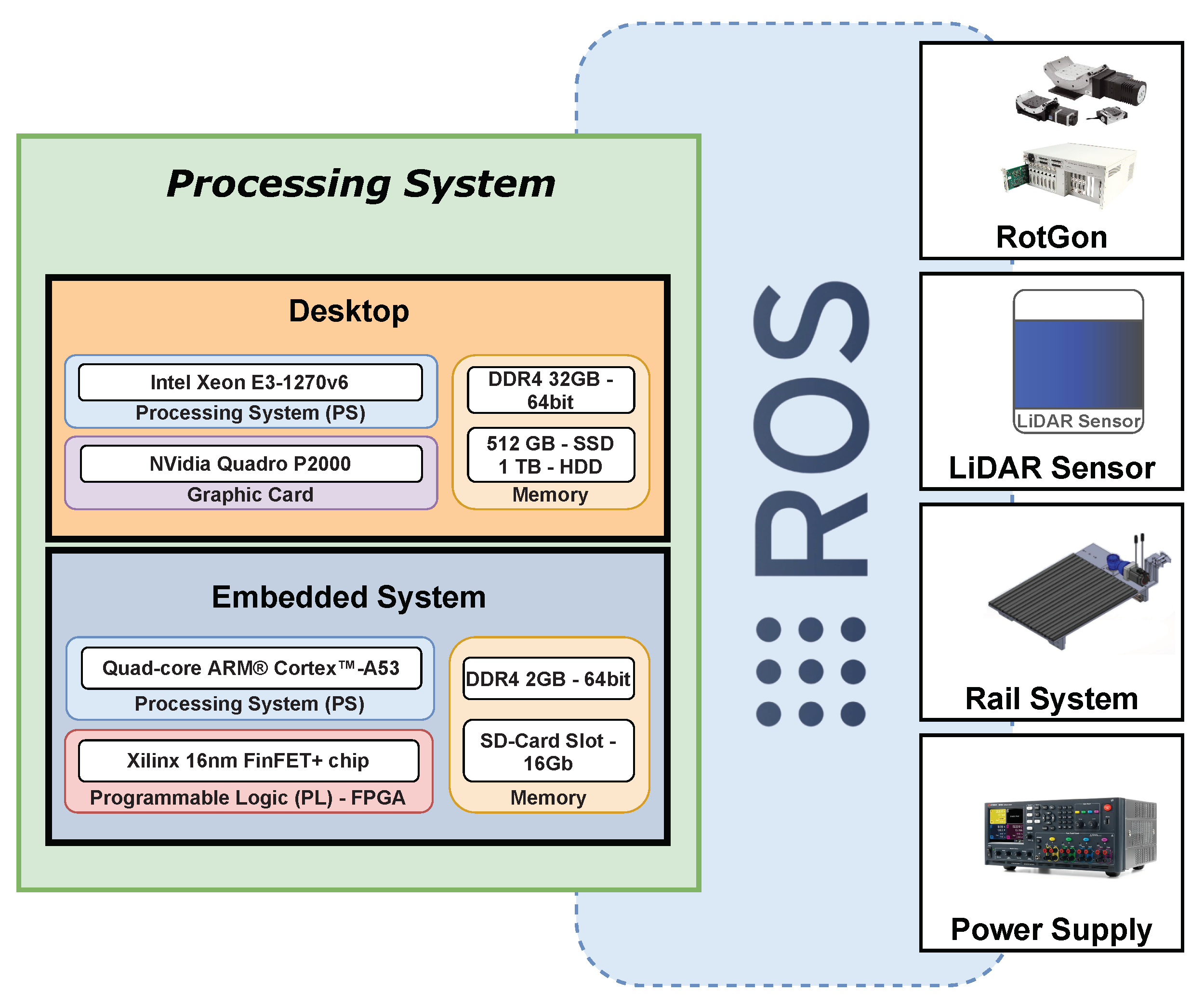
3.1. System Architecture

The Optical Lab is composed of a set of equipment used to perform the desired tests. For the FoV, AR, and short-range measurements, we use a customized rail system and goniometric rotation system (RotGon) composed of a URS150BPP Rotation Stage and an M-BGM200BPP Goniometer from Newport. Regarding the power consumption, we use a direct current (DC) power analyzer (the N6705C four-channel station), while for the external illumination influence we use an independent setup, which is further explained below. Except for the backlight interference test, the testing and evaluation platform, the architecture of which is depicted by Figure 5, connects all the equipment within a Robot Operating System (ROS) environment. All the processing tasks are distributed between a workstation and an embedded platform with acceleration capabilities through available field-programmable gate array (FPGA) technology. Either can ensure the complete system’s functionality, allowing the laboratory to perform tests with either one of the systems alone or with both at the same time, with latter approach enabling redundancy capabilities in the testing system.

The workstation is a great solution for developing testing algorithms and other computing-intensive software tasks without being concerned about hardware resources. It is composed of a powerful desktop processor, a high-performance graphics card, and 32 gigabytes of random-access memory (RAM). Due to their heavy processing requirements, certain workstation tasks can be performed by either the available processing units or by the combination of processors and the graphics card. Despite this solution, and having in mind minimal setup and hardware resources, the testing sequences and algorithms are supported by an embedded system built upon the Zynq UltraScale+ XCZU7EV-2FFVC1156 MPSoC (available in the ZCU104 Evaluation Kit). This MPSoC features a processing system (PS) that includes a quad-core Arm Cortex-A53 application processor, a dual-core Cortex-R5 real-time processor, a Mali-400 MP2 graphics processing unit, a 4KP60 capable H.264/H.265 video codec, programmable logic (PL) with FPGA technology, and 2 GB of DDR4 memory. The embedded system allows for exploration of the available FPGA for accelerating heavy processing tasks, which can help in mitigating the overall processor’s workload and avoid utilization of the workstation. This can be useful in tests that require moving equipment as well. For the purpose of this article, all evaluations were performed only with the workstation; however, this does not affect the overall behavior of the system.

3.2. Lab Equipment

• RotGon: The RotGon enables tilting/rotating of LiDAR sensors in three distinct angles. The rotation stage permits continuous 360° motion with a maximum speed of 2°/s and a minimum incremental motion of 0.01°. The goniometer allows an angular range between −15° and 45° and features a worm mounted rotary encoder for improved accuracy and repeatability. Due to its high precision, the RotGon is highly important for the measurement of the AR and the FoV.
• Rail System: The rail system was designed to enable a base moving that can handle weights of up to 30 kg and can be programmed by external communication. In turn, the base can support several targets with different reflectivity values. The rail system’s structure has a length of 25 m and it is installed inside the laboratory. Figure 6 depicts the rail system with the LiDAR sensor installed on top of the RotGon (left side) and the moving platform with a mounted target at the end of the rail structure (right side). The rail system allows the velocity and acceleration/deceleration of the moving target to be controlled with given values (in mm/s for velocity and ± mm/s² for acceleration/deceleration). Prior to its utilization, the rail system was calibrated with rangefinder equipment used to measure several distances to a target with 95% reflectivity mounted on the rail system. These measurements were used as reference values for the internal position detector sensor.
• Power Supply: This equipment is used to power and monitor the power consumption of the LiDAR sensor under test. The power supply used in the evaluation and testing platform is the N6705C DC Power Analyzer, which includes four independent channels that can be used to power and monitor four different connected modules. The voltage and current levels for each channel can be changed in real time, allowing further testing of the sensor’s behaviour under different power source conditions.
• External illumination influence (background and sunlight): Ambient light from the sun and artificial sources represents one of the major drawbacks of using LiDAR in outdoor applications. For this reason, we created the setup depicted in Figure 7, which allows the influence of the external illumination to be tested by artificially changing the behaviour of the target’s background light.

Creating a setup with uniform illumination hitting the entire target is not feasible for objects with a larger area, as this would require an extremely strong light source and it would be hard to manipulate which specific area of target should be hit by the light. Therefore, this setup includes a beam splitter between the LiDAR and the target, which can couple the light source in the receiving path coming from the target. This setup makes it particularly easy to simulate different target reflectivities by varying the sending/receiving light signal, and it is possible to specify which region overlays the background light on the receiving path. The distance from the beam splitter to the target is around 5 m, and that from the beam splitter to the LiDAR is 15 cm. The light source used is a MAGIS 650 W lamp from Desisti.

Figure 8 shows the impact of the background light on LiDAR performance. The validation of this setup was carried out with the Velodyne VLS-128; it can easily be seen that it is possible to blind the LiDAR sensor in such a way that the target is no longer detected on the point cloud. This setup allows for testing of different LiDAR systems in different illumination conditions to evaluate the impact on the collected point cloud.

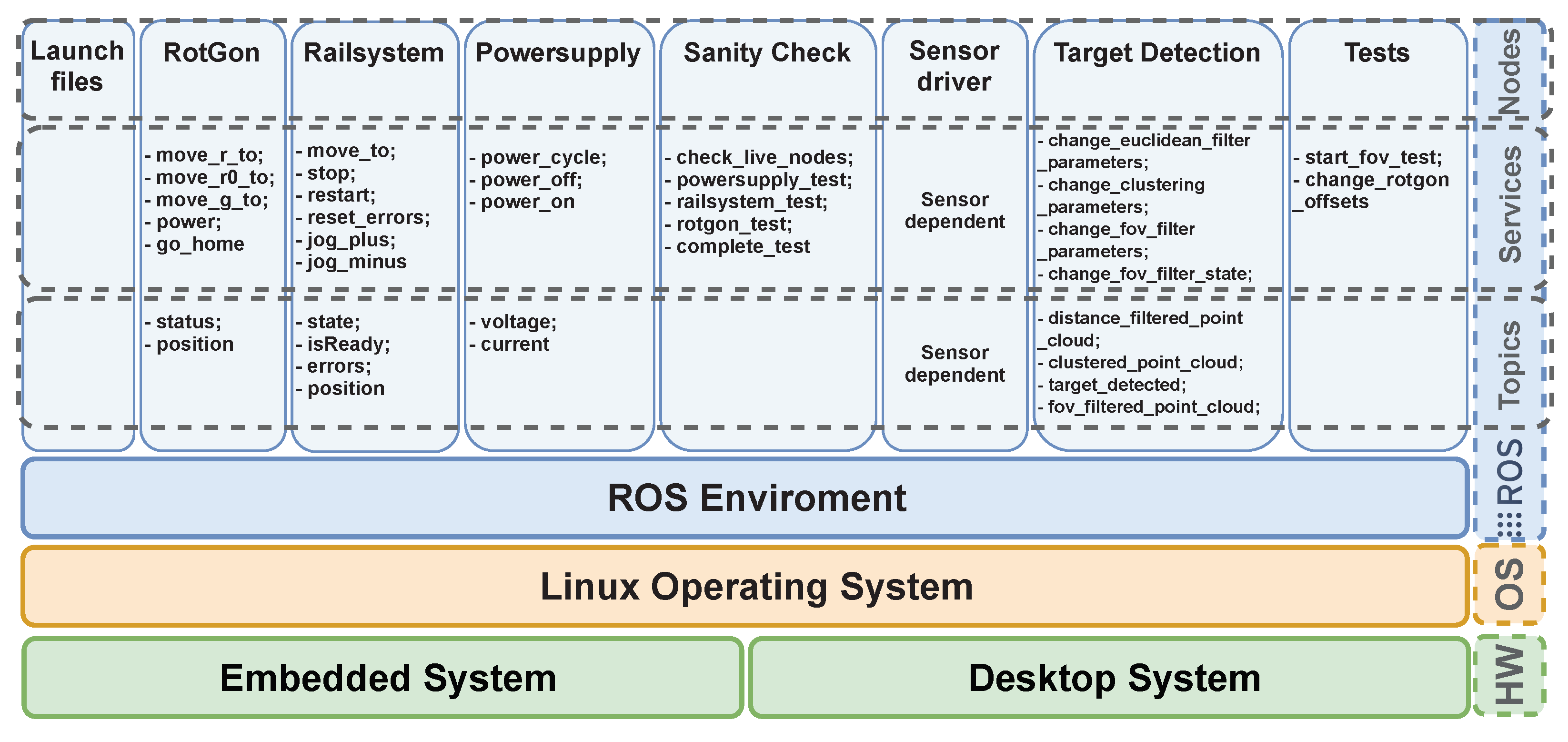
3.3. ROS Software Architecture

The system’s software stack is based on an ROS environment on top of a Linux operating system (OS), with both supported by the embedded system and the workstation. Despite each distribution being different for each platform (due to hardware resource asymmetry, processor architectures, etc.), the combination of Linux and ROS creates the required abstraction layer to develop software packages regardless of their target platform. Alongside the required ROS core components, our software architecture is composed of eight software packages, as depicted by Figure 9.

• Launch files package: This package was developed to ease the system’s launch with the correct testing setup. It allows for flexible debug sessions with different LiDAR sensors, different sensor configurations, and several system setups in which one or more components (e.g., RotGon, the rail system) may not be used. This package only presents launch files without services or topics available.
• RotGon: The RotGon package enables tilting/rotating of LiDAR sensors in three distinct angles. Therefore, this package provides three services, one for each axis, to move the sensor to the desired position/angle: move_r_to, move_r0_to, and move_g_to. Additionally, it provides a self-reset service that moves all axes to the 0${}^{\circ }$ degree position: go_home, as well as a power service to turn the device on and off. The RotGon package publishes information on two topics: one to display the current RotGon status regarding errors (status) and another to output the current angle position in real time (position).
• Railsystem: This package is responsible for moving the target within the sensor’s FoV. Therefore, it provides three moving services: one to send the target to a desired position, move_to; one to move the target away from the sensor at a constant speed and acceleration, jog_plus; and another to move the target towards the sensor, jog_minus. All can be interrupted by calling the stop service. Two more services are available: one to control the system regarding errors (reset_errors) and another to handle communication issues (restart). As with RotGon, this package has two other topics, one with status information (state) and another that publishes the current platform’s position (position).
• Powersupply: This package is responsible for controlling the sensor’s power source. It provides three services to individually control each channel: one for turning on the power source, power_on; one for turning off the power source, power_off; and another for resetting the power supply, power_cycle. In addition, it can set different voltage and current values, providing real-time measurements of the channel powering the sensor.
• Sanity Check: This package consists of a set of tools used to verify the full operation of the main system used for testing a sensor, i.e., the rail system, RotGon, and power supply. It provides one service to individually test each core component, <equipment>_test; one that tests the connectivity with the nodes, check_live_nodes; and another that sequentially tests the whole setup.
• Sensor driver: This package depends on the sensor that is currently under test. Because most manufacturers provide an ROS-based driver and packages to interface with their sensors, the evaluation and testing platform can easily support a broad number of devices. Nonetheless, each driver package has to be manually installed and configured before changing the sensor and any test configuration.
• Target detection: This package is required for tests that depend on the target’s visibility inside the sensor’s FoV, and consequently its visibility in the point cloud. It supports a set of services that are used to enable and configure several filters applied to the point cloud, such as the target’s distance, the software-based FoV, etc. Such filters are further explained in the next section. This service can output several topics with the filtered point clouds (one per filter) and one topic that continuously informs it of whether the target is inside the sensor’s FoV (target_detected).
• Tests: The Tests package contains the supported tests for the evaluation and testing platform that require the utilization of at least one of the pieces of equipment mentioned above. For each test, e.g., FoV and AR, a service is used to trigger the automated execution of the whole procedure. During the test, all the test outputs are saved in an ROS log file.

4. System Implementation

For the sake of simplicity, this section only describes the software-based filters that can be applied to a point cloud and the approaches used to calculate the FoV and the AR. The remaining tests, e.g., sensor range and point cloud acquisition (with and without background illumination), are beyond the scope of this article.

4.1. Point Cloud Filtering for Target Detection

The evaluation and testing platform aims to support any COTS LiDAR sensor as well as Bosch prototypes under development. Regarding the supported tests, e.g., FoV, target detection can be challenging because not all sensors provide the point’s intensity values along with their coordinate data. Therefore, and in order to support all sensors’ outputs, we have created a set of filters that can be used to detect targets without relying on the point intensity values, including distance and clustering filters.

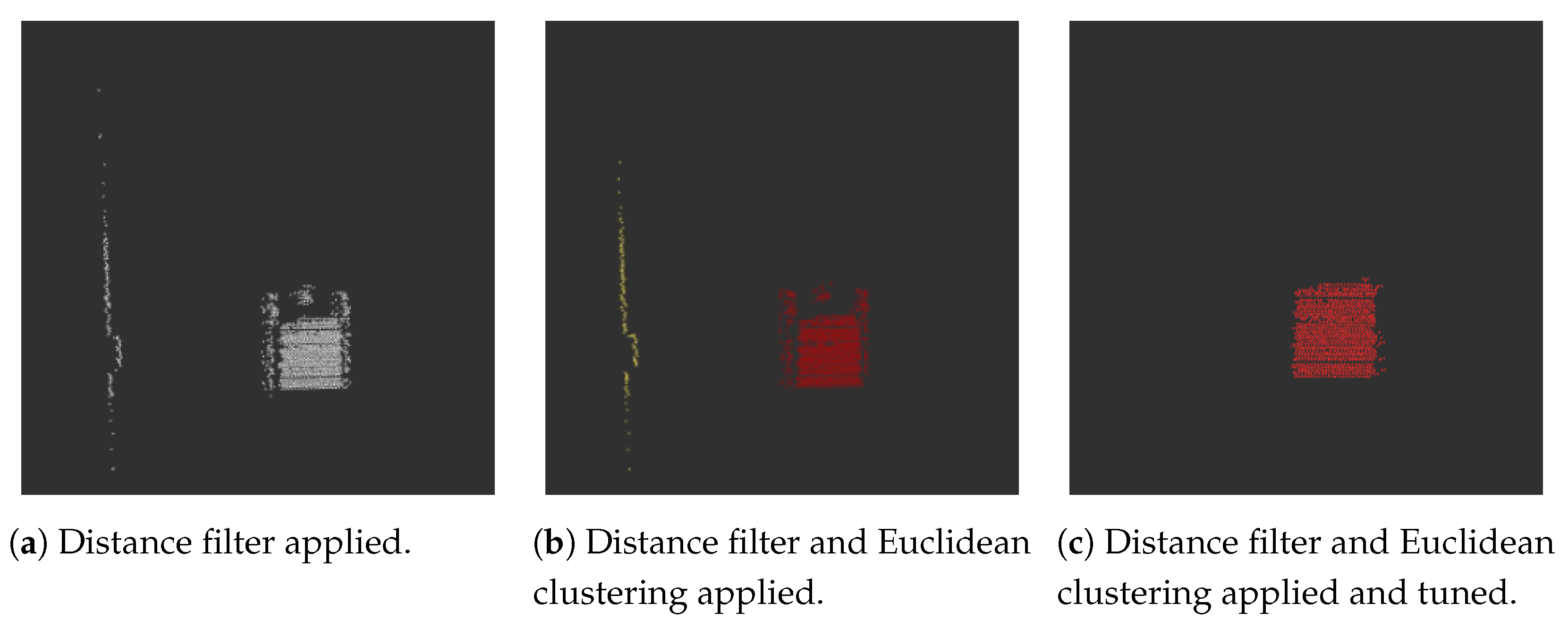
• Distance Filter (DF): Because the target is placed at a known distance from the sensor, the output of this filter is a new point cloud (published to the filtered_point_cloud topic) containing points that are, at this distance, ± a threshold value (used to avoid removal of points that actually belong to the target). The result after applying the distance filter is shown in Figure 10a. This procedure removes undesired points, and can help to reduce the computational costs of subsequent tasks.
• Clustering Filter (CF): The cluster filter algorithm groups the points that are present in the point cloud and evaluates whether the target is within the clusters created. Because the target’s distance and size and the sensor’s resolution can have an effect on the clustering results, this algorithm must be tuned afterwards. Figure 10b depicts the output of the CF algorithm without tuning its parameters; it can be seen that two clusters were identified, represented by the yellow and red points. The points present inside the yellow cluster result from points that are at the same distance as the target, which must be removed during the next step. To detect whether the resulting clusters represent the target, a Euclidean clustering filter is applied. Because the point density within the target’s cluster is higher than in other objects at the same distance, this filter analyzes the neighbour points of each point within a defined search radius $R1$. If a neighbor point is inside this search radius $R1$, it belongs to the same cluster and is retained in the point cloud; otherwise, it is removed. This task is performed by resorting to the EuclideanClusterExtraction.extract method presented in the point cloud library (PCL) [36]. The parameters used to configure this method are:
  • Cluster Tolerance: Defines the search radius $R1$; if the chosen value is too small, the same target can be divided into multiple clusters. On the other hand, multiple objects can be set as just one cluster if this value is too high. This parameter permits an interval value between 0.01 and 1 m.
  • Minimum Cluster Size: This parameter is used to define the minimum number of points required to form a cluster. It permits values between 1 and 10,000 points.
  • Maximum Cluster Size: This parameter defines the maximum number of points used to form a cluster. It supports a minimum of 2 and a maximum of 50,000 points.

Figure 10c depicts the point cloud output after applying the tuned Euclidean clustering filter. When the target’s cluster is found, this filter publishes a message to the target_detected topic using the TargetInfo message type, which contains a boolean variable (True if the target is being detected and False otherwise) and the number of points inside the cluster. The new point cloud, which now contains only the target’s cluster, is published in the clustered_point_cloud topic, which can finally be used in testing the sensor parameters, e.g., FoV and AR.

• FoV software filter (FoVSF): The purpose of this filter is to enable support for any LiDAR sensor on the market, including the rotation-based COTS LiDAR sensors widely used in automotive applications, which usually provide a 360° horizontal FoV. Notwithstanding this, for the purposes of testing and validating the platform, which must support additionally LiDAR sensors with a limited FoV, the FoV software filter allows the point cloud to be cropped to a desired horizontal and vertical FoV. This filter runs in two steps: first, it converts the points in the point cloud from the Cartesian to the spherical coordinate system, using Equation (3) to calculate the azimuth and Equation (4) for the elevation angle; in the second step, the algorithm discards the points from the point cloud that are not within the desired thresholds. The output of this filter is an ROS topic with a new point cloud containing the points that are within the configured FoV. Later, in Section 5, we present an application of this filter.

  $$\theta =\left\{\begin{array}{cc}\frac{arctan\frac{y}{x}\times 180}{\pi },\hfill & \mathrm{if}x\ge 0\mathrm{and}y\ge 0\hfill \\ \frac{arctan\frac{y}{x}\times 180}{\pi }+180,\hfill & \mathrm{if}x<0\mathrm{and}y\ge 0\hfill \\ 270-\frac{arctan\frac{y}{x}\times 180}{\pi },\hfill & \mathrm{if}x<0\mathrm{and}y<0\hfill \\ \frac{arctan\frac{y}{x}\times 180}{\pi }+360,\hfill & \mathrm{otherwise}\hfill \end{array}\right.$$

  (3)

  $$\phi =\left\{\begin{array}{cc}90-\frac{arctan\frac{\sqrt{x^2+y^2}}{z}\times 180}{\pi },\hfill & \mathrm{if}z>0\hfill \\ -(\frac{arctan\frac{\sqrt{x^2+y^2}}{z}\times 180}{\pi }+90),\hfill & \mathrm{if}z<0\hfill \\ 0,\hfill & \mathrm{otherwise}\hfill \end{array}\right.$$

  (4)

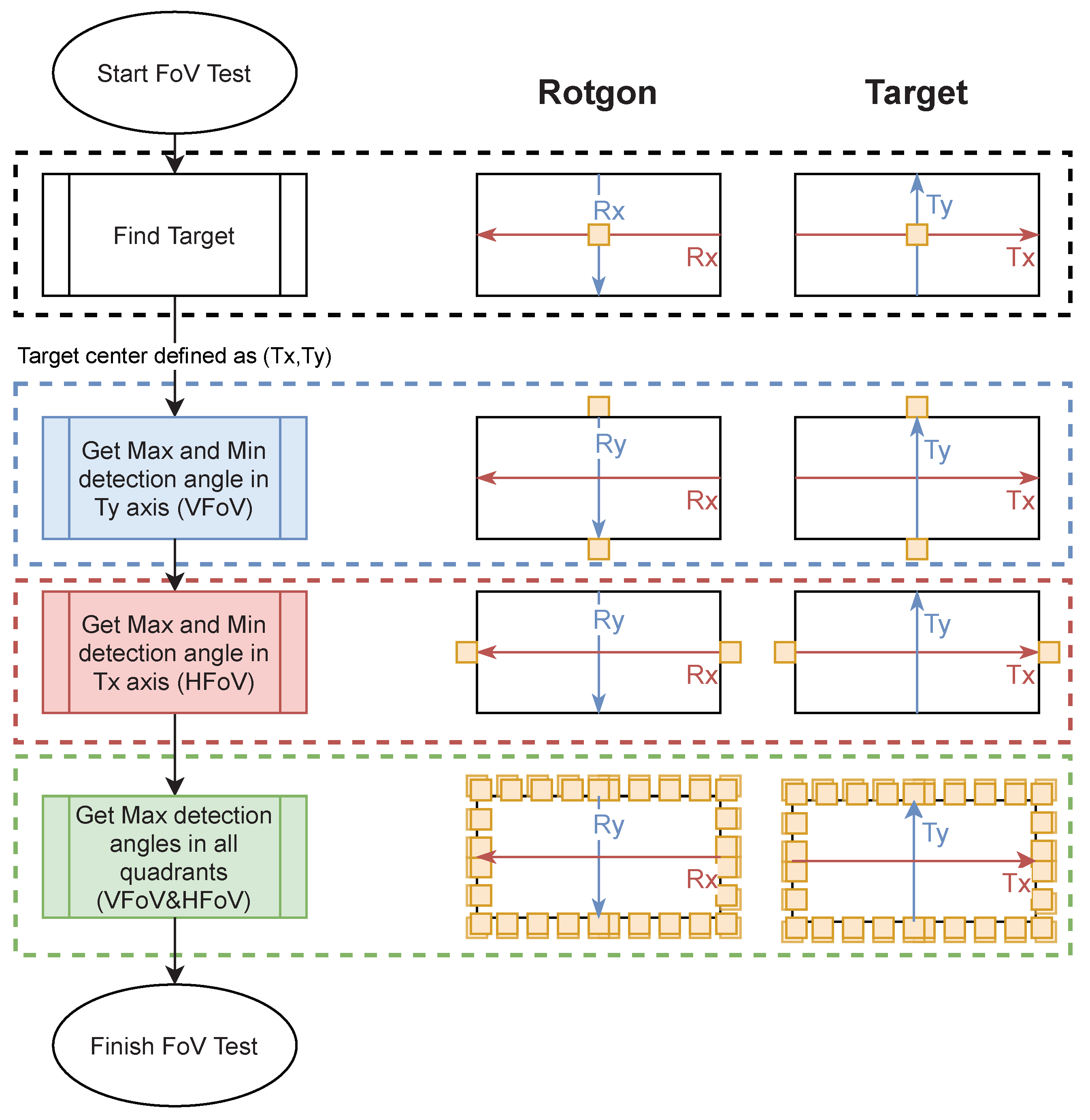
4.2. Implementation of the FoV Test

The test to determine the sensor’s FoV consists of using a target with a well-known size and reflectivity placed at a known distance on top of the rail system’s target holder. Because the rail system can only provide variable ranges, it is possible to take advantage of the RotGon to move the sensor in both the horizontal and vertical directions while checking when the target moves outside of the sensor’s FoV. Using the position data from the RotGon, it is possible to find the sensor’s FoV. The procedure is illustrated in Figure 11.

The test starts with a routine that uses the services provided by the Target Detection package described above to find a target inside the sensor’s point cloud data. If the target is detected, the algorithm starts measuring the FoV. First, it starts by finding the maximum and minimum angles in the vertical axis to achieve the vertical FoV (the blue square in the image). Next, the same concept is applied to the horizontal axis to find the horizontal FoV (the red square in the image). Finally, the values retrieved in the previous tasks are used as the starting conditions to test the consistency of both the horizontal and vertical FoVs in the limits of all quadrants (the green square in the image).

$$\begin{array}{cc}\hfill & Fo{V}_1=P1-P3\hfill \\ \hfill & Fo{V}_2=P2-P4\hfill \\ \hfill & FoV=\frac{Fo{V}_1+Fo{V}_2}{2}\hfill \\ \hfill & Fo{V}_{min}=\frac{P1+P2}{2}\hfill \\ \hfill & Fo{V}_{max}=\frac{P3+P4}{2}\hfill \end{array}$$

(5)

In all procedures, in order to obtain the maximum and minimum detection angles, the system increments/decrements the RotGon angles until the target reaches the four different positions illustrated in Figure 12:

• P1—Last position where the target is completely outside of the FoV;
• P2—First position where the target is completely inside of the FoV;
• P3—Last position where the target is completely inside of the FoV;
• P4—First position where the target is completely outside of the FoV after P3;

Then, based on Equation (5), the minimum detection angle ($Fo{V}_{min}$), maximum detection angle ($Fo{V}_{max}$), and FoV are calculated for each axis. Because this method uses the mean values of two known positions to achieve the minimum and maximum values, the target size is automatically removed from the calculations. Moreover, and in order to calculate an FoV as close as possible to the real value, at the limits of the FoV (where the target starts to disappear) we use the lowest angular step provided by the RotGon, which is 0.01°.

4.3. Implementation of the AR Test

A sensor’s AR defines the distance (in degrees) between two consecutive measured points. A smaller distance and higher number of collected points per frame represent better AR performance on the part of a sensor. With this in mind, the most straightforward way to calculate the AR of a LiDAR output is by first counting the number of points present in the point cloud (obtained from a high-reflectivity target with a known size $T_{width}\times T_{height}$, as in Figure 13, and placed at a known distance $T_{dist}$). Next, the AR can be calculated using Equation (6):

$$\begin{array}{cc}\hfill A{R}_h& =\frac{2arcsin\left(\frac{T_{width}}{2T_{dist}}\right)}{H_{number\_points}}\hfill \\ \hfill A{R}_v& =\frac{2arcsin\left(\frac{T_{height}}{2T_{dist}}\right)}{V_{number\_points}}\hfill \end{array}$$

(6)

Based on the trigonometric functions that relate the right-angled triangle created by half the size of the target ($\frac{T_{width}}{2}$ or $\frac{T_{height}}{2}$) to the distance between the sensor and the target ($T_{dist}$), it is possible to calculate the angle needed to detect half of the target. Then, the AR can be achieved by dividing this angle by the half the number of points within the target. As in the FoV test, the AR test re-measures the vertical and horizontal AR at different target positions. However, such positions are not the same as in the FoV test. There, the goal was to find the RotGon angles at which the target was entirely inside or outside the point cloud. For the AR test, the goal is to obtain multiple positions, as illustrated by Figure 14, where the angular resolution can be different.

Moreover, and because a sensor usually presents higher point density in the center of the point cloud, the AR can vary by several tenths of degrees depending on the target position. Therefore, this measurement is performed within different regions (defined by a software FoV filter) inside the point cloud, which are reduced by 25% with each iteration (Figure 14). After computing both the vertical and horizontal AR for each target position, the test summarizes the information by calculating the arithmetical mean of each virtual FoV based on Equation (7). For each iteration, we define nine positions: the central position that is common for all virtual FoVs, all four vertices, and the center of each of the four edges.

$$\begin{array}{cc}\hfill A{R}_{h_{a\%}}& =\frac{1}{9}\left(\sum _{i=1}^{9}A{R}_{h_{Pia\%}}\right)\hfill \\ \hfill A{R}_{v_{a\%}}& =\frac{1}{9}\left(\sum _{i=1}^{9}A{R}_{v_{Pia\%}}\right)\hfill \end{array}$$

(7)

5. Results

To validate the evaluation and testing platform and the algorithms developed for testing LiDAR sensors, we selected the Velodyne VLS-128, which is one of the highest-resolution sensors available on the market. This sensor is designed for specifically for autonomous vehicles. The testing setup was that depicted earlier in Figure 6. This simple test can show the full functionality of the system, as it uses most of the equipment available inside the laboratory (the RotGon, rail system, and power supply) and the software point cloud filtering modules previously discussed (DF, CF, and FoVSF). To provide reliable, precise, and accurate measurements, all equipment was previously calibrated, and to ensure the proper operation of the evaluation and testing platform, we ran a sanity check sequence before testing the sensor. For the sake of simplicity, this section only shows the setup that we created to test the FoV of a COTS LiDAR sensor.

5.1. Sanity Check

The sanity check sequence independently tests the power supply, the rail system, and the RotGon. It is provided by the Sanity Check package, which provides four main services: powersupply_test, railsystem_test, rotgon_test, and complete_test. Before running the sanity check procedure, each service uses the check_live_nodes service to checks whether the ROS node corresponding to the equipment being tested is turned on and visible within the ROS network. Regarding the outcome of the sanity checks, the test either results in success, meaning that the system is ready to test the LiDAR sensor, or in failure, in which case it reports which component resulted in an error. The errors reported by each equipment’s node are summarized in

Table 1. Sanity check error list.

Equipment	Result	Description
	1	No problems detected
Powersupply	2	No node detected in the ROS Environment
	3	Values detected not matching the expected values
	1	No problems detected
	2	No node detected in the ROS Environment
	3	Component not ready
Railsystem	4	Component has internal errors
	5	Component not moving after a moving command
	6	Component not stopping after a stop command
	7	Component not in the correct position
	1	No problems detected
Rotgon	2	No node detected in the ROS Environment
	3	Component not in the correct position

.

• Power supply sanity check: After checking whether the powersupply_node is alive, this test verifies whether any sensor is connected to the system by obtaining the list of connected sensors. Then, it evaluates whether each connected sensor’s parameters match the values reported by the power supply. There are three possible outcomes: (1) the node is unresponsive; (2) the connected sensor matches the configured parameters; or (3) the power supply readings do not match the expected values.
• Rail system sanity check: Similar to the power supply, the rail system routine begins by testing whether its corresponding ROS node is alive. Next, the rail system is validated by sending the platform that holds the target into different positions while checking the system’s response. In this way, two dedicated services are defined, move_sequence and is_moving; the first is responsible for calling the move_to services, while the latter checks whether the target is in fact moving or is at the desired position. The rail system sanity check has six possible outputs: (1) no problems were detected; (2) the node is unresponsive; (3) the node’s internal flags indicate a busy state, i.e., the rail system is not ready to receive commands; (4) the internal flags indicate internal error status; (5) the target did not move after a move_to command; (6) the target could not stop after a stop command; and (7) the target is not at the expected position.
• RotGon sanity check: This routine verifies four moving commands: go_home, move_r_to, move_r0_to, and move_g_to. Next, it tests whether the moving parts (one for each axis) are at the desired angles. This test can report three possible situations: (1) the RotGon is alive and running; (2) The RotGon node is unresponsive; and (3) the RotGon positions are different from the expected positions.

5.2. FoV Test

To validate the FoV testing algorithm, we used different FoV values within the range of the Velodyne VLS-128: a horizontal FoV of 360° and a vertical FoV of 40°. This can be adjusted by using FoVSF, provided by the Target Detection package. It is important to mention that we forced this step in order to prove the functionality of the FoVSF (mostly for the horizontal plane, as the VLS-128 provides a 360° horizontal FoV), which may not be required when testing sensors with limited FoV values and is required to validate the parameters provided and set by the manufacturer. After placing the target at a known distance and within the visibility of the configured FoV, the DF is applied to remove the points in the point cloud that are outside of the desired range, resulting in a cleaner point cloud and helping to reduce the computational requirements of the subsequent tasks. Finally, the CF step is applied. At this point, the system has successfully locked the target and is finally able to evaluate the FoV value that is known and was previously set.

The results are published in real time to the target_detected topic, which is subscribed to by the running test script, in this case corresponding to the FoV test script. Figure 15 depicts all the steps performed to detect and lock the target in the point cloud: (1) Figure 15a shows the raw data sent by the VLS-128; (2) Figure 15b depicts the application of the FoVSF; (3) Figure 15c illustrates the DF output; and (4) Figure 15d shows only the point cluster that corresponds to the target visible and locked in the point cloud.

Next, we run the Tests package, which is responsible for the algorithms previously described in Figure 11 and Figure 12. The gathered results obtained using the parameters described in

Table 2. Filter parameters.

Cluster Filter			Distance Filter		Target
Cluster Tolerance	Cluster Size (min)	Cluster Size (max)	Threshold (min)	Threshold (max)	Distance
0.03 m	100 pt	2000 pt	5.5 m	5.6 m	5.5 m

are summarized in

Table 3. Test results for the FoV evaluation.

		Horizontal FoV (min)	Horizontal FoV (max)	Vertical FoV (min)	Vertical FoV (max)
Test 1	FoVSF	0°	60°	−10°	15°
	Measured FoV	0.03°	59.89°	−1.95°	14.89°
Test 2	FoVSF	20°	75°	−15°	0°
	Measured FoV	20.02°	74.89°	−14.79°	−1.05°
Test 3	FoVSF	0°	135°	0°	17°
	Measured FoV	−1.08°	134.70°	0.04°	16.92°

. We performed three distinct tests, Test 1, Test 2, and Test 3, consisting of changing the sensor’s FoV and validating the configured values. For the vertical FoV, we measured different regions inside the original sensor’s values (40°), as this area is within the range of the RotGon’s rotation angles. For the horizontal FoV, we used three different values: 60°; 55°; and 135°.

Comparing the measured FoV values with the FoVSF parameters, makes it possible to observe the deviations of angles from the expected values and the readings from the RotGon. In the performed tests, these values ranged from 0.02° (Test 2, min. Horizontal FoV) to 0.30° (Test 3, max. Horizontal FoV). This could be for three main reasons: (1) the smallest angle the RotGon can read is 0.01°; (2) the sensor is being evaluated from the receiver’s perspective, which is only based on analyzing the received point cloud; and (3) because a CF is being applied to the target’s region in the point cloud, the number of points that belong to the cluster usually varies, which is mainly related to the sensor’s precision, accuracy, and resolution.

In all the results, the proper operation of the evaluation and testing platform is apparent, with certain calculated angles having slight deviations from the desired values. It is important to mention that our measurements are performed from the sensor receiver’s perspective, and are only based on the point cloud data provided by the sensor for use by other (high-level) applications within the perception system of the car. Therefore, we consider these deviations to not be critical at this order of magnitude; they can be used to validate the sensors’ parameters being tested. When more accurate analysis is required, it is possible to submit the sensor to an end-of-line testing scenario, which is part of the laboratory responsible for testing sensors under development within other Bosch projects. However, end-of-line testing for the laser transmitter is beyond the scope of this article.

6. Conclusions

This article presents an evaluation and testing platform that is able to test and validate different parameters of LiDAR sensors designed for automotive applications. The platform was built upon a set of equipment supported by an ROS software environment. Because the purpose of this platform is to evaluate any LiDAR sensor available on the market, we have created several ROS packages to control and automate the tests and a set of software-based filters able to support any sensor’s output based only on point cloud data information. Despite all tests being performed from the sensor receiver’s perspective, the results are quite promising. We validated the output of a Velodyne VLS-128 sensor, as well as the concept of our point cloud filtering approaches to the FoV, distance, and point clustering. Nonetheless, the current algorithms must be improved upon in order to provide more detailed information about the parameters being tested. Future developments should include more testing scenarios and parameters, such as the laser emitting power, beam divergence, spot size and shape, point cloud acquisition at different distances, maximum range, and many more. It is our goal to support tests in real-life environments as well, such as under adverse weather or in direct sunlight.

References

1. Daily, M.; Medasani, S.; Behringer, R.; Trivedi, M. Self-Driving Cars. Computer 2017, 50, 18–23. [Google Scholar] [CrossRef] [Green Version]
2. Badue, C.; Guidolini, R.; Carneiro, R.V.; Azevedo, P.; Cardoso, V.B.; Forechi, A.; Jesus, L.; Berriel, R.; Paixão, T.M.; Mutz, F.; et al. Self-driving cars: A survey. Expert Syst. Appl. 2021, 165, 113816. [Google Scholar] [CrossRef]
3. Gao, C.; Wang, G.; Shi, W.; Wang, Z.; Chen, Y. Autonomous Driving Security: State of the Art and Challenges. IEEE Internet Things J. 2022, 9, 7572–7595. [Google Scholar] [CrossRef]
4. Yurtsever, E.; Lambert, J.; Carballo, A.; Takeda, K. A Survey of Autonomous Driving: Common Practices and Emerging Technologies. IEEE Access 2020, 8, 58443–58469. [Google Scholar] [CrossRef]
5. Litman, T. Autonomous Vehicle Implementation Predictions; Victoria Transport Policy Institute Victoria: Victoria, BC, Canada, 2021. [Google Scholar]
6. Society of Automotive Engineers (SAE). Taxonomy and Definitions for Terms Related to Driving Automation Systems for On-Road Motor Vehicles (Surface Vehicle Recommended Practice: Superseding J3016 Jun 2018); SAE International: Warrendale, PA, USA, 2021. [Google Scholar]
7. Guerrero-Ibáñez, J.; Zeadally, S.; Contreras-Castillo, J. Sensor Technologies for Intelligent Transportation Systems. Sensors 2018, 18, 1212. [Google Scholar] [CrossRef] [PubMed] [Green Version]
8. Marti, E.; de Miguel, M.A.; Garcia, F.; Perez, J. A Review of Sensor Technologies for Perception in Automated Driving. IEEE Intell. Transp. Syst. Mag. 2019, 11, 94–108. [Google Scholar] [CrossRef] [Green Version]
9. Shahian Jahromi, B.; Tulabandhula, T.; Cetin, S. Real-Time Hybrid Multi-Sensor Fusion Framework for Perception in Autonomous Vehicles. Sensors 2019, 19, 4357. [Google Scholar] [CrossRef] [Green Version]
10. Mohammed, A.S.; Amamou, A.; Ayevide, F.K.; Kelouwani, S.; Agbossou, K.; Zioui, N. The Perception System of Intelligent Ground Vehicles in All Weather Conditions: A Systematic Literature Review. Sensors 2020, 20, 6532. [Google Scholar] [CrossRef]
11. Warren, M.E. Automotive LIDAR Technology. In Proceedings of the 2019 Symposium on VLSI Circuits, Kyoto, Japan, 9–14 June 2019; pp. C254–C255. [Google Scholar]
12. Li, Y.; Ibanez-Guzman, J. Lidar for Autonomous Driving: The Principles, Challenges, and Trends for Automotive Lidar and Perception Systems. IEEE Signal Process. Mag. 2020, 37, 50–61. [Google Scholar] [CrossRef]
13. Roriz, R.; Cabral, J.; Gomes, T. Automotive LiDAR Technology: A Survey. IEEE Trans. Intell. Transp. Syst. 2022, 23, 6282–6297. [Google Scholar] [CrossRef]
14. Cunha, L.; Roriz, R.; Pinto, S.; Gomes, T. Hardware-Accelerated Data Decoding and Reconstruction for Automotive LiDAR Sensors. IEEE Trans. Veh. Technol. 2022, 1–10. [Google Scholar] [CrossRef]
15. Arnold, E.; Al-Jarrah, O.Y.; Dianati, M.; Fallah, S.; Oxtoby, D.; Mouzakitis, A. A Survey on 3D Object Detection Methods for Autonomous Driving Applications. IEEE Trans. Intell. Transp. Syst. 2019, 20, 3782–3795. [Google Scholar] [CrossRef] [Green Version]
16. Shi, S.; Wang, X.; Li, H. PointRCNN: 3D Object Proposal Generation and Detection From Point Cloud. Available online: https://openaccess.thecvf.com/content_CVPR_2019/html/Shi_PointRCNN_3D_Object_Proposal_Generation_and_Detection_From_Point_Cloud_CVPR_2019_paper.html (accessed on 1 September 2022).
17. Wu, J.; Xu, H.; Tian, Y.; Pi, R.; Yue, R. Vehicle Detection under Adverse Weather from Roadside LiDAR Data. Sensors 2020, 20, 3433. [Google Scholar] [CrossRef]
18. Wang, H.; Wang, B.; Liu, B.; Meng, X.; Yang, G. Pedestrian recognition and tracking using 3D LiDAR for autonomous vehicle. Robot. Auton. Syst. 2017, 88, 71–78. [Google Scholar] [CrossRef]
19. Peng, X.; Shan, J. Detection and Tracking of Pedestrians Using Doppler LiDAR. Remote Sens. 2021, 13, 2952. [Google Scholar] [CrossRef]
20. Huang, W.; Liang, H.; Lin, L.; Wang, Z.; Wang, S.; Yu, B.; Niu, R. A Fast Point Cloud Ground Segmentation Approach Based on Coarse-To-Fine Markov Random Field. IEEE Trans. Intell. Transp. Syst. 2022, 23, 7841–7854. [Google Scholar] [CrossRef]
21. Karlsson, R.; Wong, D.R.; Kawabata, K.; Thompson, S.; Sakai, N. Probabilistic Rainfall Estimation from Automotive Lidar. In Proceedings of the 2022 IEEE Intelligent Vehicles Symposium (IV), Aachen, Germany, 4–9 June 2022. [Google Scholar]
22. Raj, T.; Hashim, F.; Huddin, B.; Ibrahim, M.; Hussain, A. A Survey on LiDAR Scanning Mechanisms. Electronics 2020, 9, 741. [Google Scholar] [CrossRef]
23. Behroozpour, B.; Sandborn, P.A.M.; Wu, M.C.; Boser, B.E. Lidar System Architectures and Circuits. IEEE Commun. Mag. 2017, 55, 135–142. [Google Scholar] [CrossRef]
24. Jiménez, J. Laser diode reliability: Crystal defects and degradation modes. Comptes Rendus Phys. 2003, 4, 663–673. [Google Scholar] [CrossRef]
25. Kwong, W.C.; Lin, W.Y.; Yang, G.C.; Glesk, I. 2-D Optical-CDMA Modulation in Automotive Time-of-Flight LIDAR Systems. In Proceedings of the 2020 22nd International Conference on Transparent Optical Networks (ICTON), Bari, Italy, 19–23 July 2020; pp. 1–4. [Google Scholar] [CrossRef]
26. Fersch, T.; Weigel, R.; Koelpin, A. A CDMA Modulation Technique for Automotive Time-of-Flight LiDAR Systems. IEEE Sensors J. 2017, 17, 3507–3516. [Google Scholar] [CrossRef]
27. Lee, H.; Kim, S.; Park, S.; Jeong, Y.; Lee, H.; Yi, K. AVM / LiDAR sensor based lane marking detection method for automated driving on complex urban roads. In Proceedings of the 2017 IEEE Intelligent Vehicles Symposium (IV), Los Angeles, CA, USA, 11–14 June 2017; pp. 1434–1439. [Google Scholar] [CrossRef]
28. Jokela, M.; Kutila, M.; Pyykönen, P. Testing and Validation of Automotive Point-Cloud Sensors in Adverse Weather Conditions. Appl. Sci. 2019, 9, 2341. [Google Scholar] [CrossRef] [Green Version]
29. Vargas Rivero, J.R.; Gerbich, T.; Teiluf, V.; Buschardt, B.; Chen, J. Weather Classification Using an Automotive LIDAR Sensor Based on Detections on Asphalt and Atmosphere. Sensors 2020, 20, 4306. [Google Scholar] [CrossRef] [PubMed]
30. Roriz, R.; Campos, A.; Pinto, S.; Gomes, T. DIOR: A Hardware-Assisted Weather Denoising Solution for LiDAR Point Clouds. IEEE Sensors J. 2022, 22, 1621–1628. [Google Scholar] [CrossRef]
31. Chan, P.H.; Dhadyalla, G.; Donzella, V. A Framework to Analyze Noise Factors of Automotive Perception Sensors. IEEE Sensors Lett. 2020, 4, 1–4. [Google Scholar] [CrossRef]
32. Carballo, A.; Lambert, J.; Monrroy, A.; Wong, D.; Narksri, P.; Kitsukawa, Y.; Takeuchi, E.; Kato, S.; Takeda, K. LIBRE: The Multiple 3D LiDAR Dataset. In Proceedings of the 2020 IEEE Intelligent Vehicles Symposium (IV), Las Vegas, NV, USA, 19 October 2020–13 November 2020; pp. 1094–1101. [Google Scholar] [CrossRef]
33. Lambert, J.; Carballo, A.; Cano, A.M.; Narksri, P.; Wong, D.; Takeuchi, E.; Takeda, K. Performance Analysis of 10 Models of 3D LiDARs for Automated Driving. IEEE Access 2020, 8, 131699–131722. [Google Scholar] [CrossRef]
34. Suss, A.; Rochus, V.; Rosmeulen, M.; Rottenberg, X. Benchmarking time-of-flight based depth measurement techniques. In Smart Photonic and Optoelectronic Integrated Circuits XVIII; He, S., Lee, E.H., Eldada, L.A., Eds.; SPIE: Bellingham, WA, USA, 2016; Volume 9751, pp. 199–217. [Google Scholar]
35. Sun, W.; Hu, Y.; MacDonnell, D.G.; Weimer, C.; Baize, R.R. Technique to separate lidar signal and sunlight. Opt. Express 2016, 24, 12949–12954. [Google Scholar] [CrossRef]
36. Rusu, R.B.; Cousins, S. 3D is here: Point Cloud Library (PCL). In Proceedings of the 2011 IEEE International Conference on Robotics and Automation (ICRA), Shanghai, China, 18 August 2011; pp. 1–4. [Google Scholar]
Figure 1. Perception system of a car.
Applsci 12 13003 g001
Figure 2. LiDAR working principle.
Applsci 12 13003 g002
Figure 3. LiDAR horizontal and vertical FoV.
Applsci 12 13003 g003
Figure 4. LiDAR horizontal and vertical AR.
Applsci 12 13003 g004
Figure 5. System architecture.
Applsci 12 13003 g005
Figure 6. Evaluation and testing platform with the goniometric rotation system, LiDAR sensor, and the rail system.
Applsci 12 13003 g006
Figure 7. Experimental setup for background light influence.
Applsci 12 13003 g007
Figure 8. Influence of background light.
Applsci 12 13003 g008
Figure 9. Software stack overview.
Applsci 12 13003 g009
Figure 10. Target detection steps.
Applsci 12 13003 g010
Figure 11. Field of view flowchart overview.
Applsci 12 13003 g011
Figure 12. Target positions for FoV measurement.
Applsci 12 13003 g012
Figure 13. Points reflected by a known target.
Applsci 12 13003 g013
Figure 14. Target positions for full AR evaluation.
Applsci 12 13003 g014
Figure 15. Target detection steps.
Applsci 12 13003 g015