Prediction of Suzhou’s Industrial Power Consumption Based on Grey Model with Seasonal Index Adjustment

Abstract

The accurate prediction of industrial power consumption is conducive to the effective allocation of power resources by power and energy institutions, and it is also of great significance for the construction and planning of the national grid. By analyzing the characteristics of the data of Suzhou’s industrial power consumption between 2003 and 2005, this paper proposes a grey model with a seasonal index adjustment to predict industrial power consumption. The model results are compared with the traditional grey model, as well as the real value of Suzhou’s industrial power consumption, which shows that our model is more suitable for the prediction of industrial power consumption. The lasted Suzhou’s industrial power consumption data, from 2019–2021, are also investigated, and the results show that the prediction results are in very good agreement with the real data. The highlights of the paper are that all precision inspection indexes are excellent and the seasonal fluctuations in the data changes can be reflected in the present model.

1. Introduction

Industrial power consumption is an important part of the power consumption of the whole society and the economic dispatching of the power system. With the rapid development of the industrial economy, the consumption of industrial power is also growing at a fast pace, and the proportion of industrial power consumption in the whole society is also increasing. Due to the fact that electric energy cannot be stored and used on a large scale, the accurate prediction of industrial power consumption will effectively improve the reasonable allocation of power resources [1,2,3].

In the research of power demand forecasting, an increasing number of scholars have integrated forecast methods into practices. Yang applied the principle of least square filtering to analyze the monthly load data of the power system, established a mathematical model, and realized the load forecast of the domestic power system for the first time [4]. Ding et al. proposed a curve extrapolation method based on curve mode analysis for an online mode extrapolation algorithm of ultra-short term load forecasting [5]. Furthermore, he also focused on the practical problems, such as the historical bad data processing, based on this method and the special processing of current load level, which has strong applicability. Pan et al. used the radial basis function (RBF) as the kernel function of the support vector machine (SVM) prediction method to establish the mathematical model [6]. The model is applied to forecast the daily load of the power system in a city located in Jiangsu Province, China. Kandil et al. took the data of the Quebec hydropower station as an example and proposed a simple multi-layered feed-forward artificial neural networks (ANN) model [7], which can interpolate among the load and weather variables pattern data of training sets to provide the future load pattern of the Hydro-Quebec. Fan et al. developed a load forecast method based on an adaptive two-stage hybrid network with self-organizing map (SOM) and SVM, and applied it to analyzing the data of the historical energy load from the New York Independent System Operator [8]. Xiang et al. took wavelet transform to extract the periodic and nonlinear characteristics of power load, decomposed the power load sequence into subsequences of different frequency bands, and used an artificial neural network model make predictions according to the characteristics of each subsequence [9]. Qin et al. predicted the future regional growth in electricity and weight function using the electric elasticity coefficient method [10]. Shi et al. established a multiple regression model based on the screening of economic leading indicators and predicted monthly electricity consumption in Anhui Province from May 2014 to December 2014 [11]. Cui et al. adopted the ARIMAX model based on co-integration relation theory to exploit self-relevant information of the internal sequence, as well as the correlation between sequences [12]. This model has a high value under the presence of a mutation structure and significant influence factors in the short-term load forecasting field. Shi et al. established a hybrid model for short-term load forecasting, which combined the adaptability of Kalman filter forecasting on the basis of the time series analysis forecasting method [13]. Zhang et al. combined the merits of ANN and grey prediction to develop a novel load forecasting method, named grey neural network (GNN), and applied it to the monthly load demand forecasting of Shandong Province [14]. Li et al. found that the model combining the random forest algorithm with the weak time series could achieve good results in predicting the time of future power load data [15]. Alani et al. developed a near-zero cooperative probabilistic scenario analysis and decision tree (PSA-DT) model to address the lacuna of an enormous predictive error faced by the state-of-the-art models [16]. Chen et al. established an industrial power consumption prediction model and used residual error and posterior error to test the accuracy of the model [17]. Lv et al. solved the problem faced by a single algorithm by using the grey model to fit the nonlinear growth trend of power load, and the time series model to characterize the seasonality and periodicity of the load [18].

Traditional prediction methods include the trend extrapolation method, elastic coefficient method, regression analysis method, time series method, Kalman filtering method and grey theory prediction method [19,20,21,22,23,24]. Li et al. applied a trend extrapolation method to study the power load and found the prediction results of the second-order adaptive coefficient were better than that of quadratic exponential smoothing [19]. Meng used the elastic coefficient method to predict the electricity quantity and load of the Qitaihe area [20]. In order to predict the irregular charging energy demand, Mir et al. advanced a short-term load forecasting method through regression analysis [21]. Sopelsa Neto et al. presented a fault prediction method based on enhanced time series forecasting models, which could evaluate the development of the fault before a flashover occurs [22]. Dawood implemented a short-term prediction of energy consumption based on a standard Kalman filter [23]. Yan proposed a grey GM(1, n) model for predicting the short-term power load [24].

Modern prediction methods include the support vector machine, artificial neural network, wavelet analysis, random forest, decision tree [25,26,27,28,29], etc. Moradzadeh et al. proposed a hybrid support vector regression algorithm and, through it, performed a short-term load forecasting in a Microgrid [25]. Arvanitidis et al. used an artificial neural network to obtain the consumption data of the Greek interconnected power system [26]. Branco et al. predicted the fault in electrical power grids by a long short-term memory model based on wavelet transform [27]. Dudek et al. carried out short-term load forecasting using the random forest method [28]. Ding used decision the tree method to clarify the relationship between the load and the relative variables and implement a long-term load forecasting [29].

Based on the current research, we found that most of the prediction models have combined two or more prediction methods to obtain useful information. However, it is still difficult to find an accurate prediction method that can be applied to any region and any situation. This is because the real system is complex and diverse, and it will also be affected by many external factors, such as economy, policy, climate and holidays. In this paper, we analyze the characteristics of Suzhou’s industrial power consumption data and set up a grey model with a seasonal index adjustment to predict the industrial power consumption.

The remaining parts of this paper are organized as follows. Section 2 analyzes the data of Suzhou’s industrial power consumption between 2003 and 2005 and finds its characteristics. Section 3 introduces the grey model with a seasonal index adjustment. Section 4 discusses the empirical analysis results of Suzhou’s industrial power consumption. The conclusion is given in Section 5.

2. Characteristic Analysis of Industrial Power Consumption

The industrial power consumption data used in this paper are from the official website of the Suzhou Bureau of Statistics [30]. A total of 36 data sets of “Industrial Power Consumption” in “Transportation and Power consumption”, between the years 2003 and 2005, are selected as the research object. The monthly time series of each year is shown in Figure 1. It can be seen that there are two typical characteristics: (1) Seasonal fluctuation. The data curves representing the three years in Figure 1 basically maintain the same distribution characteristics: in each year, the trough appears in February and October, respectively, and the peak appears in July and December. In particular, the data in January and February 2004 changed significantly. According to the survey, the Spring Festival of China is usually in February, while the Spring Festival of 2004 took place in January, and the climate change in January and February also had an impact on power consumption. This shows that the industrial power consumption in Suzhou has the periodic characteristics of seasonal fluctuations. (2) Trend growth. The data of power consumption in the same month over three years are compared, which shows that they have an obvious growth trend.

According to the typical characteristics of Suzhou’s industrial power consumption, this paper proposes a forecasting method of a grey model with a seasonal index adjustment. In the following sections, the seasonal index is introduced; then, the grey model is established; finally, the forecast results are inversely adjusted by the seasonal index.

3. Grey Model with Seasonal Index Adjustment

Seasonal index is a method based on statistics used to reveal the seasonal variation of time series data. As the data used in this paper have the characteristics of periodic change, the moving average method is used to smooth the fluctuations of the original number series, separate the seasonal index, and obtain a stable smooth series without seasonal fluctuations. Then, based on the stationary smooth sequence, a prediction model is established to obtain the simulation value. Finally, we need to multiply the simulation value by the seasonal index to restore its seasonal fluctuation.

3.1. Seasonal Index Model

In this subsection, the seasonal index model is set up. Supposing the original sequence is $x^{(0)}=\left\{x_1^{(0)},x_2^{(0)},\cdots x_n^{(0)}\right\}$ and N is a certain number of time interval terms, which is usually consistent with the length of seasonal variation, such as four quarters or 12 months, the specific steps of a seasonal index model are as follows:

(1) The moving average of the original sequence is $x^{(1)}=\left\{x_1^{(1)},x_2^{(1)},\cdots ,x_m^{(1)}\right\}$, where $x_m^{(1)}$ can be calculated from the simple equation:

$$x_m^{(1)}=\frac{0.5x_m^{(0)}+x_{m+1}^{(0)}+\cdots +x_{m+N-1}^{(0)}+0.5x_{m+N}^{(0)}}{N},m=1,2,\cdots ,n-N$$

(1)

(2) Calculate the ratio C of each period by:

$$C_{i+N/2}=\frac{x_{i+N/2}^{(0)}}{x_i^{(1)}}\times 100\%,i=1,2,\cdots ,n-N$$

(2)

(3) Calculate the seasonal index SI by:

$$S{I}_j=\raisebox{1ex}{$N{\overline{C}}_j$}\!\left/ \!\raisebox{-1ex}{${\displaystyle \sum {\overline{C}}_j}$}\right.,j=1,2,\cdots ,N$$

(3)

where ${\overline{C}}_j$ is the average value of the ratio of different time intervals in the same period.

3.2. Grey Model

The grey model is usually applied to an atypical process in which the factors constituting the system are not completely clear and very little information is known. The model combines the characteristics of differential equation and difference equation, which can better describe the internal characteristics and development trends of and the sequence and make scientific quantitative predictions.

Given $y^{(0)}=\left\{y_1^{(0)},y_2^{(0)},\cdots y_n^{(0)}\right\}$ as the modeling sequence, it can obtain the one time accumulation generating sequence $y^{(1)}=\left(y_1^{(1)},y_2^{(1)},\cdots ,y_n^{(1)}\right)$, where $y_n^{(1)}={\displaystyle {\displaystyle \sum }_{i=1}^n}{y}_i^{\left(0\right)}$, $y_i^{(0)}>0$. Suppose z⁽¹⁾ is the nearest mean generating the sequence of y⁽¹⁾, which can be written as $z_k^{(1)}=0.5y_k^{(1)}+0.5y_{k-1}^{(1)}$, $k=2,3,\cdots ,n$, then the basic form of the GM (1, 1) grey differential model is:

$$-a{z}_k^{\left(1\right)}+b=y_k^{\left(0\right)},k=2,3,\cdots ,n$$

(4)

where parameters a and b can be obtained by the least square method. The matrix form of Equation (4) can be given by $Y=B\cdot u$, in which $Y={(y_2^{\left(0\right)},y_3^{\left(0\right)},\cdots ,y_n^{\left(0\right)})}^T$, $u={(a,b)}^T$ and $B=\left[\begin{array}{cc}-z_2^{\left(1\right)}& 1\\ -z_3^{\left(1\right)}& 1\\ ⋮& ⋮\\ -z_n^{\left(1\right)}& 1\end{array}\right]$.

In the Equation (4), if k is regarded as a continuous variable t, $y^{(1)}$ can be written as $y_t^{(1)}$; let $y_t^{(0)}$ correspond to $\frac{d{y}_t^{(1)}}{dt}$, and $z_t^{(1)}$ correspond to $y_t^{(1)}$, an albino differential equation $\frac{d{y}_t^{(1)}}{dt}+a{y}_t^{(1)}=b$ can be established; suppose the initial value ${\widehat{y}}_1^{(1)}=y_1^{(0)}$, and the prediction model can be derived from:

$${\widehat{y}}_{t+1}^{(1)}=\left(y_1^{(0)}-\frac{b}{a}\right)e^{-at}+\frac{b}{a},t=0,1,2,\cdots$$

(5)

The accumulated prediction equation can be given by:

$${\widehat{y}}_{t+1}^{(0)}={\widehat{y}}_{t+1}^{(1)}-{\widehat{y}}_t^{(1)},t=1,2,\cdots$$

(6)

3.3. Prediction Steps of Grey Model with Seasonal Index Adjustment

The grey model with a seasonal index adjustment uses the seasonal index to adjust the original number series, then uses the grey model to fit the data development trend, and finally uses the seasonal index reverse adjustment to restore the seasonal fluctuations of the data. The main prediction steps are as follows:

(1) Calculate the seasonal index. Calculate the data according to Equations (1)–(3) to obtain seasonal index.

(2) Data preprocessing. Divide the original sequence by the seasonal index, we can obtain a group of smooth sequence $x^{(2)}=\left\{x_1^{(2)},x_2^{(2)},\cdots ,x_i^{(2)},\cdots x_n^{(2)}\right\}$, which is a stationary smooth sequence without seasonal fluctuations. The $x_i^{(2)}$ can be given by:

$$x_i^{(2)}=x_i^{(0)}/SI$$

(7)

(3) Model calculation. We use the new sequence $x^{(2)}$ as the modeling sequence $y^{(0)}$ of the grey model, establish the grey prediction model, and obtain the prediction sequence ${\widehat{y}}^{(0)}$.

(4) Data recovery. We use the seasonal index to make a reverse adjustment. That is, the grey prediction sequence ${\widehat{y}}^{(0)}$ is multiplied by the seasonal index $SI$ to obtain the simulation value ${\tilde{x}}^{(0)}$, where ${\tilde{x}}^{(0)}$ is as follows:

$${\tilde{x}}^{(0)}={\widehat{y}}^{(0)}\times SI$$

(8)

3.4. Model Accuracy Inspection

Prediction model tests generally include an errors test, correlation test and posterior error test. In this subsection, we define these tests and list the reference of accuracy inspection grade.

(1)

Errors test

The errors are defined as absolute error ${\Delta }^{\left(0\right)}\left(i\right)=\left|x^{(0)}\left(i\right)-{\tilde{x}}^{\left(0\right)}\left(i\right)\right|$, relative error $e\left(i\right)=\frac{{\Delta }^{\left(0\right)}\left(i\right)}{x^{(0)}\left(i\right)}$, and average relative error (ARE) $\overline{e}=\frac{1}{n}{\displaystyle \sum _{i=1}^{n}e\left(i\right)}$.

(2)

Correlation test

Based on the absolute error, the minimum level difference is ${\Delta }_{\min }=\underset{i}{\min }\underset{k}{\min }{\Delta }_i\left(k\right)$, the maximum level difference is ${\Delta }_{\max }=\underset{i}{\max }\underset{k}{\max }{\Delta }_i\left(k\right)$, and the calculation formula of the correlation coefficient is $\xi \left(k\right)=\frac{{\Delta }_{\min }+\zeta {\Delta }_{\max }}{\Delta \left(k\right)+\zeta {\Delta }_{\max }}$, in which $\zeta$ is the resolution coefficient with the value between 0 and 1. The larger the value of $\zeta$, the larger the value of the correlation, generally $\zeta =0.5$. Grey correlation degree (GCD) is defined as $r=\frac{1}{n}{\displaystyle \sum _{k=1}^n\xi \left(k\right)}$.

(3)

Posterior error test

A posteriori error test is carried out according to the mean variance ratio and small error probability. Mean variance ratio (MVR) is defined as $C=\frac{S_2}{S_1}=\sqrt{\frac{{{\displaystyle \sum \left[{\Delta }^{\left(0\right)}\left(i\right)-{\overline{\Delta }}^{\left(0\right)}\right]}}^2}{n-1}}/\sqrt{\frac{{{\displaystyle \sum \left[x^{\left(0\right)}\left(i\right)-{\overline{x}}^{\left(0\right)}\right]}}^2}{n-1}}$, where ${\overline{x}}^{\left(0\right)}=\frac{1}{n}{\displaystyle {\displaystyle \sum }_{i=1}^n}{x}_i^{(0)}$ and ${\overline{\Delta }}^{\left(0\right)}=\frac{1}{n}{\displaystyle {\displaystyle \sum }_{i=1}^n}{\Delta }_i^{(0)}$. Small error probability (SEP) is defined as $P=P\left\{\left|{\Delta }^{\left(0\right)}\left(i\right)-{\overline{\Delta }}^{\left(0\right)}\right|<0.6745S_1\right\}$.

According to the literature [31], the accuracy inspection grade is shown in

Table 1. Reference of accuracy inspection grade.

	Index	ARE	GCD	MVR	SEP
Grade
I		0.01	0.90	0.35	0.95
II		0.05	0.80	0.50	0.80
III		0.10	0.70	0.65	0.70
IV		0.20	0.60	0.80	0.60

.

4. Empirical Analysis

4.1. Data Source

In this paper, we selected the 36 month monthly data of Suzhou’s industrial power consumption between the years 2003 and 2005 as the sample data and built the original sequence. These data are shown in

Table 2. Monthly data of industrial power consumption in Suzhou from 2003 year to 2005 year.

Year	Jan	Feb	Mar	Apr	May	Jun	Jul	Aug	Sep	Oct	Nov	Dec
2003	22.17	17.80	23.90	22.87	23.20	24.64	29.38	29.06	26.71	25.97	28.19	30.25
2004	22.65	27.81	31.05	30.36	31.18	32.95	36.41	35.30	33.02	33.72	35.97	36.42
2005	36.21	27.38	35.96	37.09	39.17	43.06	46.85	44.87	42.27	40.53	42.69	47.49

.

4.2. Solving Seasonal Index

It can be seen from Table 2 that the n = 36 and N = 12 in the original sequence. Substituting them into Equation (1), we can obtain the average sequence $x^{(1)}$ = $\{$25.37, 25.80, 26.52, 27.13, 27.77, 28.45, 29.09, 29.64, 30.17, 30.75, 31.40, 31.98, 32.80, 33.35, 33.54, 34.02, 34.63, 35.39, 36.24, 37.08, 37.86, 38.53, 39.10, 39.84$\}$. According to Equation (2), the ratio of each period is C = $\{$115.81, 112.64, 100.72, 95.72, 101.51, 106.33, 77.86, 93.83, 102.92, 98.73, 99.3, 103.03, 111.01, 105.85, 98.45, 99.12, 103.87, 102.91, 99.92, 73.84, 94.98, 96.26, 100.18, 108.08$\}$. Compared with the original sequence, the number of sequence items of the average sequence is N/2 less at the beginning and end. Therefore, the corresponding period of ratio sequence C is from July 2003 to June 2005. For the positive period, we can obtain the average ratio $\overline{C}$ = $\{$88.89, 83.84, 98.95, 97.50, 99.74, 105.56, 113.41, 109.25, 99.59, 97.42, 102.69, 104.62$\}$ from January to December. Then, the seasonal index (SI) is calculated according to Equation (3), which is shown in

Table 3. Seasonal index of monthly industrial power consumption.

Time	SI	Time	SI
Jan	0.8878	Jul	1.1327
Feb	0.8374	Aug	1.0912
Mar	0.9883	Sep	0.9947
Apr	0.9738	Oct	0.9730
May	0.9962	Nov	1.0257
Jun	1.0543	Dec	1.0449

.

4.3. Data Preprocessing

Using the seasonal index in Table 3 and Equation (7), we can seasonally adjust the original sequence and obtain a new sequence $x^{(2)}=$ $\{$24.97, 21.26, 24.18, 23.48, 23.29, 23.37, 25.94, 26.63, 26.85, 26.69, 27.48, 28.95, 25.51, 33.21, 31.42, 31.18, 31.30, 31.25, 32.14, 32.35, 33.20, 34.66, 35.07, 34.85, 40.79, 32.70, 36.39, 38.09, 39.32, 40.84, 41.36, 41.12, 42.50, 41.65, 41.62, 45.45$\}$. By comparing the new sequence with the original sequence data, it can be seen that the new sequence data are smoother and show an upward growth trend (see Figure 2).

4.4. Grey Modeling Calculation

Take the new sequence as the modeling sequence, build the GM (1, 1) grey model, and substitute it into Equation (4), we can obtain $\left[\begin{array}{cc}-z_2^{\left(1\right(}& 1\\ -z_3^{\left(1\right)}& 1\\ ⋮& ⋮\\ -z_n^{\left(1\right)}& 1\end{array}\right]\left(\begin{array}{c}a\\ b\end{array}\right)=\left[\begin{array}{c}{x}_2^{\left(2\right)}\\ x_3^{\left(2\right)}\\ ⋮\\ x_n^{\left(2\right)}\end{array}\right]$, and the model parameters a = −0.0193 and b = 22.4643. Substitute the parameters into Equation (5) and obtain the prediction model ${\widehat{y}}_{k+1}^{(1)}=1190{.64\mathrm{e}}^{0.0193k}-1165.67$. In this model, take $k=0,1,2,\cdots ,n-1$ in turn to obtain the results. The calculation result is substituted into Equation (6) for cumulative calculation, then we can obtain the prediction sequence ${\widehat{x}}^{(2)}$ = $\{$24.97, 23.17, 23.62, 24.08, 24.55, 25.02, 25.51, 26.01, 26.51, 27.03, 27.56, 28.09, 28.64, 29.20, 29.76, 30.34, 30.93, 31.54, 32.15, 32.77, 33.41, 34.06, 34.73, 35.40, 36.09, 36.79, 37.51, 38.24, 38.98, 39.74, 40.51, 41.30, 42.11, 42.93, 43.76, 44.61$\}$.

4.5. Data Recovery

Substituting the prediction sequence ${\widehat{x}}^{(2)}$ into Equation (8) for reverse adjustment, that is ${\tilde{x}}^{(0)}={\widehat{x}}^{(2)}\times S$, we can obtain the final result of the model ${\tilde{x}}^{(0)}$ =$\{$22.17, 19.40, 23.34, 23.45, 24.46, 26.38, 28.90, 28.38, 26.37, 26.30, 28.27, 29.35, 25.43, 24.45, 29.41, 29.55, 30.81, 33.25, 36.42, 35.76, 33.23, 33.14, 35.62, 36.99, 32.04, 30.81, 37.07, 37.24, 38.83, 41.90, 45.89, 45.07, 41.89, 41.77, 44.88, 46.61$\}$.

4.6. Results and Discussion

In order to verify the effectiveness of the present prediction method, the grey model without a seasonal index adjustment (i.e., the traditional GM (1, 1)) is used as Model 1, and the grey model with a seasonal index adjustment is used as Model 2. The simulation results and accuracy test results of both models are compared.

(1)

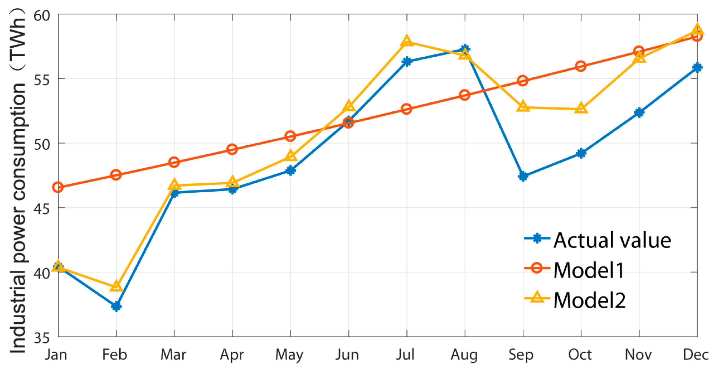
Comparison of simulation results

Figure 3 shows the comparison between the actual values and the simulation results of both models. It can be seen that the simulation result of Model 1 displays a relatively smooth curve, which cannot effectively reflect the fluctuation characteristics of the actual value; the simulation result of Model 2 is well consistent with the actual value.

(2)

Errors test

Figure 4 shows the relative error of both models. It can see that the relative error of Model 2 is significantly reduced, and the average relative error of Model 2 decreases, from 0.0657 to 0.0337, in comparison to Model 1. In terms of the errors test, the simulation effect of Model 2 is better.

(3)

Correlation test

The actual value is taken as the reference sequence, and Model 1 and Model 2 are taken as the comparison sequence. By calculating this, we can obtain the minimum range ${\Delta }_{\min }=0$ and the maximum range ${\Delta }_{\max }=9.82$. According to the calculation formula of the GCD, we can obtain the values of the GCD, which are 0.7587 and 0.8500 in Model 1 and Model 2, respectively; therefore, the precision of Model 2 is higher than that of Model 1.

(4)

Posterior error test

By calculating the mean variance ratio (MVR) and small error probability (SEP) formulae, we can ascertain that the MVR is C = 0.2751 and the SEP is P = 0.9722 in Model 1, and the MVR is C = 0.1353 and the SEP is P = 1 in Model 2. According to Table 1, both Model 1 and Model 2 have reached Grade 1; however, the precision of Model 2 is higher than Model 1, so the method of the grey model with a seasonal index adjustment is more effective. From the calculation results and inspection results, the accuracy of the four indicators of Model 2 achieve or are close to Grade I, and its simulation values effectively reflect the actual seasonal fluctuations of industrial power consumption.

(5)

Comparison of forecast results

In order to further verify the effectiveness of the present model, it is used to predict the industrial power consumption in 2006 and compare it with the actual value. The results are shown in Figure 5 and the accuracy related index results are shown in

Table 4. Precision index of Models 1 and 2 in 2006 year.

Index	ARE	GCD	MVR	SEP
Model 1	0.096	0.5827	0.4466	0.8333
Model 2	0.038	0.7728	0.2748	1

.

It can be seen from Figure 5 and Table 4 that Model 2 is better than Model 1. In Figure 5, the curve of Model 2 is very close to the actual value in the first eight months, but there is some error in the data from September to December. According to the chronicle of events in Suzhou of 2006 year, we found that there was a major policy adjustment in the Suzhou’s Industrial Park in September 2006, which led to certain fluctuations in the industrial power consumption. It is therefore evident that Model 2 can reflect the real fluctuation. Table 4 shows that the data of the four precision indicators of the prediction values of Model 2 are also excellent. According to the judgment of the accuracy inspection grade shown in Table 1, we find that the ARE has achieved Grade II, the GCD has achieved Grade III, and the MVR and SEP have achieved Grade I, which indicates that the grey model with a seasonal index adjustment proposed in this paper has certain effectiveness in forecasting industrial power consumption.

(6)

Model application expansion

We have investigated the Suzhou’s industrial power consumption data of 2003–2005 from our previous project, which shows that the prediction results of the present model are excellent. In order to further verify the extrapolation capability of this present model, we also investigate the latest Suzhou’s industrial power consumption data from 2019–2021. The comparison between the simulation results and the actual values is shown in Figure 6. It can be seen that the simulation results are in very good agreement with the real data, particularly in terms of the fluctuation. We also calculate the ARE and GCD, which are 0.0496 and 0.8658, respectively. The MVR is C = 0.2116 and the SEP is P = 1. According to the judgment of the accuracy inspection grade shown in Table 1, the four indicators are excellent.

5. Conclusions

In this paper, we have analyzed the monthly data of industrial power consumption in Suzhou between the years 2003 and 2005. According to its characteristics of seasonal fluctuation and trend growth, we proposed a forecasting method using the grey model with a seasonal index adjustment. The highlights of the present method are that it combines the advantages of the seasonal index model and the grey model, which not only effectively used the grey model to describe the internal characteristics and development trend of the data, but also skillfully introduced the seasonal index to adjust the original sequence, seasonally, to eliminate the influence of seasonal factors and reversed the seasonal adjustment of the predicted value with the seasonal index after the prediction. The results show that the present model is more suitable for the prediction of industrial power consumption because it is superior to the traditional grey model in terms of all precision inspection indexes, the fitting and prediction values, and it can also effectively reflect the seasonal fluctuations of the real data. In order to further verify the extrapolation capability of the present model, we have investigated the latest Suzhou’s industrial power consumption data from 2019–2021, and the results show that the prediction results are in very good agreement with the real data. This indicates that the proposed method is effective and applicable. In further research work, we will build some new prediction methods, such as a deep learning model based on the neural network or Markov chain.

References

1. Liu, Q.; Zhang, L.; Li, J.; Zhang, C.; Tan, X.; Zhang, K.; Guo, W. Study on the trend of China’s electricity consumption during the “14th Five Year Plan”. Electr. Power 2022, 55, 214–219. [Google Scholar] [CrossRef]
2. Wang, X.; Zhu, B.; Gu, Z. Mid-and-long term load forecasting based on integrated power consumption data. Electric Power 2021, 54, 211–216. [Google Scholar] [CrossRef]
3. Yun, Z.; Quan, Z.; Caixin, S.; Shaolan, L.; Yuming, L.; Yang, S. RBF Neural Network and ANFIS-Based Short-Term Load Forecasting Approach in Real-Time Price Environment. IEEE Trans. Power Syst. 2008, 23, 853–858. [Google Scholar] [CrossRef]
4. Yang, Z. Fast prediction of power system load curve using least square filtering principle. Heilongjiang Electr. Power 1981, 4, 1–9. [Google Scholar] [CrossRef]
5. Ding, Q.; Lu, J.; Qian, Y.; Zhang, J.; Liao, H. A practical method for Ultra-short term load forecasting. Autom. Electr. Power Syst. 2004, 28, 83–85. [Google Scholar]
6. Pan, F.; Cheng, H.; Yang, J.; Zhang, C.; Pan, Z. Power system short-term load forecasting based on support vector machines. Power Syst. Technol. 2004, 28, 39–42. [Google Scholar] [CrossRef]
7. Kandil, N.; Wamkeue, R.; Saad, M.; Georges, S. An efficient approach for short term load forecasting using artificial neural networks. Int. J. Electr. Power Energy Syst. 2006, 28, 525–530. [Google Scholar] [CrossRef]
8. Fan, S.; Chen, L. Short-Term Load Forecasting Based on an Adaptive Hybrid Method. IEEE Trans. Power Syst. 2006, 21, 392–401. [Google Scholar] [CrossRef]
9. Xiang, Z.; Wang, X. Forecasting approach to short-time load using wavelet decomposition and artificial neural network. J. Syst. Simul. 2008, 20, 5018–5020. [Google Scholar] [CrossRef]
10. Qin, H.; Liu, Y.; Xiao, H.; Zheng, D.; Yang, S.; Wang, H. Forecast of medium and long-term power demand and distribution in Chongqing. Electr. Power Constr. 2015, 36, 115–122. [Google Scholar] [CrossRef]
11. Shi, X.; Ge, F.; Xiao, X. Forecasting Industrial Electricity Consumption of Anhui province based on K-L information method. Power Syst. Clean Energy 2015, 31, 58–62. [Google Scholar]
12. Cui, H.; Peng, X. Summer short-term load forecasting based on ARIMAX model. Power Syst. Prot. Control. 2015, 43, 108–114. [Google Scholar]
13. Shi, W.; Wu, K.; Wang, D.; Wang, D. Eclectic power system short-term load forecasting model based on time series analysis and Kalman filter algorithm. Tech. Autom. Appl. 2018, 37, 9–12+23. [Google Scholar]
14. Zhang, D.; Ren, Z.; Bi, Y.; Zhou, D.; Bi, Y. Power load forecasting based on grey neural network. In Proceedings of the IEEE International Symposium on Industrial Electronics, Cambridge, UK, 30 June–2 July 2008; pp. 1885–1889. [Google Scholar] [CrossRef]
15. Li, W.; Chen, H.; Guo, K.; Guo, S.; Han, J.; Chen, Y. Research on electrical load prediction based on random forest algorithm. Comput. Eng. Appl. 2016, 52, 236–243. [Google Scholar] [CrossRef]
16. Alani, A.Y.; Osunmakinde, I.O. Short-Term Multiple Forecasting of Electric Energy Loads for Sustainable Demand Planning in Smart Grids for Smart Homes. Sustainability 2017, 9, 1972. [Google Scholar] [CrossRef] [Green Version]
17. Chen, J.; Lv, H. A Study on the prediction of industrial electricity consumption in Nanjing based on discrete grey model. J. Nanjing Inst. Technol. 2018, 18, 50–54. [Google Scholar] [CrossRef]
18. Lv, X.; Pan, D.; Wang, K.; Bi, J. Markov modified grey-time series electric load forecasting method. Tech. Autom. Appl. 2022, 41, 132–136+176. [Google Scholar]
19. Li, S.; Liu, L.; Liu, Y. Application of trends extrapolation on the power load forecast. J. Shenyang Inst. Eng. 2005, 1, 64–65. [Google Scholar] [CrossRef]
20. Meng, X. Research on Power Load Forecasting and Grid Planning in Qitaihe Area. Master’s Thesis, Harbin University of Science and Technology, Harbin, China, 2020. [Google Scholar] [CrossRef]
21. Mir, A.A.; Ullah, K.; Khan, Z.A.; Bashir, F.; Khan, T.U.R.; Altamimi, A. Short Term Load Forecasting for Electric Power Utilities: A Generalized Regression Approach Using Polynomials and Cross-Terms. Eng. Proc. 2021, 12, 21. [Google Scholar] [CrossRef]
22. Neto, N.F.S.; Stefenon, S.F.; Meyer, L.H.; Ovejero, R.G.; Leithardt, V.R.Q. Fault Prediction Based on Leakage Current in Contaminated Insulators Using Enhanced Time Series Forecasting Models. Sensors 2022, 22, 6121. [Google Scholar] [CrossRef]
23. Dawood, N. Short-Term Prediction of Energy Consumption in Demand Response for Blocks of Buildings: DR-BoB Approach. Buildings 2019, 9, 221. [Google Scholar] [CrossRef] [Green Version]
24. Yan, S. Research on Short-Term Forecasting Method of Power Load Based on Grey Theory Combined with Cluster Analysis. Master’s Thesis, Shenyang Agricultural University, Shenyang, China, 2022. [Google Scholar] [CrossRef]
25. Moradzadeh, A.; Zakeri, S.; Shoaran, M.; Mohammadi-Ivatloo, B.; Mohammadi, F. Short-Term Load Forecasting of Microgrid via Hybrid Support Vector Regression and Long Short-Term Memory Algorithms. Sustainability 2020, 12, 7076. [Google Scholar] [CrossRef]
26. Arvanitidis, A.I.; Bargiotas, D.; Daskalopulu, A.; Laitsos, V.M.; Tsoukalas, L.H. Enhanced Short-Term Load Forecasting Using Artificial Neural Networks. Energies 2021, 14, 7788. [Google Scholar] [CrossRef]
27. Branco, N.W.; Cavalca, M.S.M.; Stefenon, S.F.; Leithardt, V.R.Q. Wavelet LSTM for Fault Forecasting in Electrical Power Grids. Sensors 2022, 22, 8323. [Google Scholar] [CrossRef]
28. Dudek, G. A Comprehensive Study of Random Forest for Short-Term Load Forecasting. Energies 2022, 15, 7547. [Google Scholar] [CrossRef]
29. Ding, Q. Long-term load forecast using decision tree method. In Proceedings of the 2006 IEEE PES Power Systems Conference and Exposition (PSCE’06), Atlanta, GA, USA, 29 October 2006; pp. 1541–1543. [Google Scholar]
30. Suzhou Bureau of Statistics. Available online: http://tjj.suzhou.gov.cn/sztjj/tjyx/nav_list_4.shtml (accessed on 1 October 2022).
31. Cao, J.; Xiao, L.; Cheng, T. Mathematical Modeling and Mathematical Experiment, 2nd ed.; Xi’an University of Electronic Science and Technology Press: Xi’an, China, 2018. [Google Scholar]
Figure 1. Industrial power consumption of Suzhou.
Applsci 12 12669 g001
Figure 2. Comparison the new sequence with original sequence.
Applsci 12 12669 g002
Figure 3. Comparison the actual values with the simulation results of models 1 and 2.
Applsci 12 12669 g003
Figure 4. Comparison of relative error of both models.
Applsci 12 12669 g004
Figure 5. Comparison the simulation results with the actual values in 2006.
Applsci 12 12669 g005
Figure 6. Comparison the simulation results with the actual values in 2019-2021.
Applsci 12 12669 g006