Abstract
The key to intelligent traffic control and guidance lies in accurate prediction of traffic flow. Since traffic flow data is nonlinear, complex, and dynamic, in order to overcome these issues, graph neural network techniques are employed to address these challenges. For this reason, we propose a deep-learning architecture called AMGC-AT and apply it to a real passenger flow dataset of the Hangzhou metro for evaluation. Based on a priori knowledge, we set up multi-view graphs to express the static feature similarity of each station in the metro network, such as geographic location and zone function, which are then input to the multi-graph neural network with the goal of extracting and aggregating features in order to realize the complex spatial dependence of each station’s passenger flow. Furthermore, based on periodic features of historical traffic flows, we categorize the flow data into three time patterns. Specifically, we propose two different self-attention mechanisms to fuse high-order spatiotemporal features of traffic flow. The final step is to integrate the two modules and obtain the output results using a gated convolution and a fully connected neural network. The experimental results show that the proposed model has better performance than eight other baseline models at 10 min, 15 min and 30 min time intervals.
1. Introduction
With the continued development of cities in recent years, people’s transportation needs have greatly increased, and urban transportation issues are becoming increasingly severe. Scientific and effective management of road congestion has become a challenging problem for traffic management departments. As an effective means of solving traffic problems, the intelligent transport system (ITS) has become a hotspot in the transport field. In smart city and intelligent transport system (ITS) development and operation, traffic status is sensed by sensors installed on the roads (such as loop detectors), transaction logs of subway and bus systems, traffic monitoring videos, and so on. A key component of ITS is traffic flow prediction. Accurately predicting traffic flow ahead of time can help travelers to manage their trips reasonably, avoid rush hour, and reduce travel times and costs. In the case of transportation operators, early intervention may improve network capacity and efficiency and reduce accidents.
The mathematical statistics-based model named historical average (HA) and the autoregressive integrated moving average (ARIMA) model have good time-series performance in the early stages, but are not proficient at predicting traffic flows [1,2]. Subsequently, machine learning and deep-learning techniques were introduced to improve the prediction accuracy. Recurrent neural networks (RNN) derived from natural language processing (NLP), which can capture non-linear relationships in the temporal dimensions of traffic flows, and gated recurrent unit network (GRU), with gate control mechanisms and long short-term memory network (LSTM), were later introduced to predict the speed and throughput of traffic [3,4]. These methods, however, consider only temporal dependencies and ignore spatial ones. CNN-based convolutional neural networks model cities as grids and traffic streams as images in order to extract spatial correlations [5], but this method can only be used for Euclidean forms of data and is not optimal for graph-based forms of transportation networks, such as metro systems and the road network [6]. Networks combining LSTM with CNNs will be able to extract spatial–temporal correlations, but RNN-based models do not use parallel computation during training, which requires longer training times, and some of the structural information of the graph is lost during pre-processing [7,8].
Graph neural networks have become the frontier of deep-learning research in recent years, showing state-of-the-art performance in a variety of data based on graph structures [9]. The existing graph convolution neural network is split into the spectral method and the spatial cube method [10]. The spectral method uses the graph convolution theorem to define graph convolution from the spectral domain, whereas the spatial method converges each central node and its adjacent nodes from the domain of nodes through a defined convolution function. Chebyhev’s spectral CNN (ChebNet) [11] uses the truncated expansion of the Chebyshev polynomial to reach order k in order to make an approximation to the diagonal matrix. GCN [12] is a first-order approximation to ChebNet, using the Chebyshev polynomial approximation filter of the diagonal matrix of eigenvalues. An alternative method is spatial graph convolution, in which graph convolution is defined by propagating information. Diffusion Graph Convolution (DGC), message passing neural network (MPNN), GraphAEGE, and graph attention network (GAT) all follow this approach [13,14,15,16]. With the development of graph neural networks, it has been found that GNN-based models can be used to simulate spatial–temporal correlations in complex traffic networks. The spatial–temporal convolution network (STGCN) [17] is an excellent model based on spectral graph convolution and gated convolution neural network. Conv-GCN combines spectral convolution with the three-dimensional convolutional neural network (3DCNN), which compensates for the inability of spectral convolution to capture spatial correlation in depth, and divides the traffic flows into near-term, daily, and weekly segments in order to extract spatial–temporal correlations [18]. Temporal Graph Convolution Network (T-GCN) combines GCN with GRU in order to extract spatiotemporal features [19]. Diffusion Convolutional Recurrent Neural Network (DCRNN) extracts spatial correlations using the stochastic wandering strategy of GCN [20]. In the multivariate time-series prediction network (MTGNN), a graph learning module is proposed to automatically extract the correlation between segments in order to improve the graph representation and make predictions [21]. Given the inadequacy of expressing a single graph, the spatial–temporal multigraph solution network (ST-MGCN) encodes pairwise non-Euclidean correlations between regions in multiple graphs, then explicitly models these correlations using multi-graph convolution, and uses recurrent contextual-gated neural networks, which augment recursive neural networks to reweight different historical observations using contextual sensor-gated mechanisms [22]. Attention-based graph neural networks are also widely used in traffic flow prediction. An example is the spatial–temporal graph attention network (AST-GAT), which uses multi-head graph attention to capture the spatial correlation between segments of a road traffic network [23].
In general, the existing models have some disadvantages. RNN-based graph neural network models, for example, typically require more loss of training time and lack robustness. Second, a single-graph neural network model cannot extract deep spatial features between the nodes of a graph. While a few studies have proposed neural networks with multiple graphs, or even the relationship between nodes learned by the model itself, the lack of a priori knowledge of the traffic means that the accuracy and robustness of predictions can still be improved.
To overcome these shortcomings, in this paper we propose a deep-learning architecture called AMGC-AT, which consists of a multi-view convolutional network and a spatiotemporal attention network. In the multi-view convolutional network module, spatial features are extracted from four different spatial adjacency matrices, which are based on different domain knowledge. In addition, the spatiotemporal attention module is composed of two attention mechanisms, which can better integrate spatiotemporal features across three time patterns. The model is evaluated with the Hangzhou Metro Passenger Flow Data Set and the results show that the model is superior to eight other baseline models in subway passenger flow prediction. The main contributions of this research are as follows:
- The AMGC-AT model proposed in this paper is based on the domain knowledge of transport and achieves a better balance between the complexity of the model framework and the comprehensive exploration of this knowledge.
- The AMGC-AT model is based on three types of traffic flow patterns (recent, daily and weekly), and innovatively combines two kinds of self-attention mechanisms in order to drill deeply into the high-order spatial temporal information of subway patronage. The features learned by the neural network can be fully expressed in a reasonable output layer configuration.
- In this study, we perform a large number of comparative and ablation experiments, which show that the AMGC-AT model outperforms the other eight base models at all time points at randomly chosen locations. The ablation experiment provides evidence for the validity and rationality of each component of the model framework.
2. Data
2.1. Dataset Description
The AMGC-AT model presented in this paper was evaluated using a real-world dataset. The dataset was the Hangzhou Metro smart-card data, published by the Tianchi Big Data Competition, for 25 days from 1 January 2019 to 25 January 2019. The data covered about 70 million metro passengers across 81 metro stations from three metro lines. The raw data, as shown in Table 1, recorded tap-in and tap-out time, line ID, device ID, user ID, and pay type. The data obtained from AFC card processing has an operating time from 06:00 to 23:30 for tap-in and outgoing station passenger flow sequence data, which is integrated into specific time intervals of 10 min, 15 min, 30 min, and progress passenger flow sequence at 10 min time granularity, as shown in Table 2. The first week passenger inflow as shown in Figure 1. The distribution map of the Hangzhou metro line as shown in Figure 2.

Table 1.
Example of original data record.
Table 2.
Example of passenger flow.
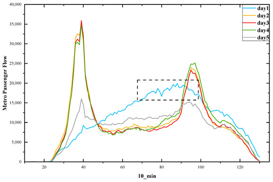
Figure 1.
First week passenger inflow.
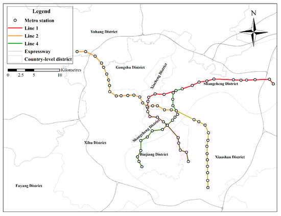
Figure 2.
Distribution of metro stations.
2.2. Dataset Preprocessing
During the raw data processing process, completely duplicated records were first removed, and the data from station entry and exit times outside the subway operating time were also removed. We then deleted the same input and output records and removed records for travel times of more than three hours as Hangzhou Metro requires a fee of $2 to stay in a station for more than 3 h, and very few riders will travel more than 3 h.
As can be seen in Figure 1, the pattern of flow volume on 1 January (the blue curve in the figure) was significantly different from that on other weekdays and weekends. This is due to the fact that peak traffic did not occur at the usual morning and evening peak traffic period and is lower than normal peak traffic. Considering the negative impact of the holiday season on projections of passenger traffic, we used only 24 days of travel data from 2 to 25 January in this paper. All data were normalized to the range (0, 1) with min–max scalers.
2.3. Problem Definition
In this section, the definitions of important symbols are introduced and the definition of the research task is formally presented.
Definition 1
(Metro Station). For a city subway system, each station serves as the spatial unit for metro passenger flow prediction. We define V = , to represent the set of subway stations, wherein n is the station number. In addition, is an adjacency matrix representing the node’s proximities between any pair of nodes.
Definition 2
(Time Interval). For the temporal dimension, the entire time period is divided into time intervals of equal length, i.e., T = ,. At each time segment, we calculate the inflow or outflow of traffic from each site at different time intervals, such as 15, 30 and 60 min.
Definition 3
(Passenger Flow). The passenger flow matrix F =, whereby n is the station number that is ordered according to the metro line number, m denotes past time intervals used to predict passenger traffic at the next time interval, and is the inflow vector in a specific time interval.
Problem 1
(Problem Statement). Given the above definitions, our research problem can be defined according to (1), whereby is the mapping function to be learnt using the proposed deep-learning framework.
3. Methodology
This section begins by describing the framework of the proposed model, followed by a step-by-step description of each component.
3.1. Overview of the Proposed Model
The AMGC-AT model architecture is shown in Figure 3. The model framework consists of two parts: the graph representation module and the traffic flow prediction module. The pictorial representation is a pre-defined set of four schemas based on a priori knowledge. Macroscopically, the predefined scheme considers location information, functional location splitting, network topology information, and the flow of traffic between stations in the metro network. The second part is intended to predict traffic volumes throughout the metro system. The system consists of a multi-view convolution module, a spatial–temporal self-attention module, and a gated convolution network. Firstly, multi-view convolution networks can capture the correlation in depth of each metro station point in space. Second, the spatiotemporal self-attention mechanism can be used to learn the dependency of spatial embeddings on different epochs of a road segment. Finally, the output goes into the complete connection layer through the gated convolution network. To reduce the dimensionality of the planar layer, we use a fully connected layer and capture the non-linear relationship between high-level features and predicted outcomes. The final step is to reconstruct the output of the full connection layer as the target shape.
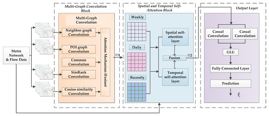
Figure 3.
Framework of Model.
3.2. Pre-Defined Affinity Graph Representation
In the macro-level graph section, we show different types of correlations among regions with multiple graphs, including: (1) the neighborhood graph which encodes the spatial proximity; (2) the SimRank graph which encodes the similarity in distant regions; (3) the Functional similarity graph which enhances the representation of spatial similarity in neighborhood graphs; (4) the Cosine similarity graph which considers the similarity of node volume at a macro level. Note that it is straightforward to extend our approach to model new types of relevance by constructing correlation graphs.
3.2.1. Neighborhood Graph
Neighborhood of a subway network is defined based on L-space modeling. Nodes represent subway points, and if two subway points are adjacent to each other on a particular line, they have a contiguous border corresponding to that line. This approach preserves the fundamental geometry of the rail network.
3.2.2. SimRank Graph
SimRank similarity between metro points is calculated as follows [24]:
where C is a constant between 0 and 1. We iterate over all in-neighbor pairs of (a, b), and sum up the similarity of these pairs. Then we divide by the total number of in-neighbor pairs, , to normalize. That is, the similarity between a and b is the average similarity between in-neighbors of a and in-neighbors of b. Note that the similarity between an object and itself is defined to be 1. This method can be used to encode similar relationships between more distant stations in the subway network.
3.2.3. Functional Similarity Graph
When a region is predicted, it is intuitively possible to refer to other regions that are functionally similar to it, and this method is also applicable for subway-network passenger-flow forecasting. Peripheral POIs of each category can be used to characterize the function of the area around the station, and the edge between two subway station points is defined as POI similarity.
where denote POI vectors of node , with dimension equal to the number of POI categories.
3.2.4. Cosine Similarity Graph
In this paper, we use cosine similarity to calculate the similarity of flow between any pair of stations in a subway network. This is a common method to obtain the similarity between two vectors.
where and are volume vectors of subway point and .
3.3. Prediction Network Module
3.3.1. Multi-Graph Convolution Module
Based on the four predefined diagrams based on a priori knowledge (presented in Section 3.2), we designed the following multi-layer spatial convolution for each representation based on spectral graph theory. The GCN model in this paper uses an efficient layered-propagation rule based on a first-order approximation of spectral convolution on a graph. Experimental results on a large network dataset show that the GCN model can encode the graph structure and node characteristics in a useful semi-supervised classifier [12]; thus, our application of this model for predicting station traffic in metro networks is reasonable and effective, and results of this research in Section 4 again confirm this.
where represents the learnable neural layer, and . where denotes the feature matrix of all metro stations. Here, denotes the feature dimension, represents the -th layer’s output. The dimension of the hidden state for the potential representation of all metro points is denoted by . Similarly, we can write the formalization of the convolution of the other three graphs.
In reality, these four representations are not completely unrelated. Therefore, we designed a generic GCN for convolution operations using parameter-sharing strategies. where ave denotes the average. We formally define the dissemination plan through the following operations:
Then we concatenate the features from the convolution of the five graphs as follows:
where att denotes the attention mechanism, represents the output feature of the GCNs. Eventually, will be entered into the output layer along with the mentioned in the next section, and the output will be the predicted target shape through the full connection layer.
3.3.2. Spatial and Temporal Self-Attention Module
In a real subway network scenario, passenger flow patterns may exhibit cyclical trends in multi-time granularity, such as time-dependence on weekly, daily, and adjacent time slots. In order to effectively capture trends in passenger flow state evolution over different periodic, three types of time intervals are coded in our model: (1) recent time intervals (e.g., trends over the first few adjacent periods of the forecast period), (2) short-term time intervals (e.g., daily trends), and (3) long-term time intervals (e.g., weekly trends). Semantic embedding of the different time intervals learned is then fed into the spatial and temporal Self-Attention Module. Formally, the formula for the temporal and spatial self-attention module is defined as follows:
Time interval-specific representations of metro stations are concatenated as Here, and represent the parametrized weight matrix of the embedding . and are two common forms of attention computing. refers to “Scaled Dot-Product Attention”, P refers to where we further embed the position into the node representation in order to segment the chronological information of the sequence. We use in order to scale the input vector, and we can prevent it from getting into saturated areas or making the gradient too small. is a shared attentional mechanism which indicate the importance of node ’s spatial features to node . And .
In this paper, is a single-layer feedforward neural network, and we further inject graphic structure into the mechanism by performing masking attention, which means only for nodes could be computed attention coefficients, where is some neighborhood of node in the L-space metro network. In addition, softmax function is used for normalization in order to make the coefficient easy to compare between nodes. Finally, the attention coefficient is passed through the LeakyReLU nonlinear function, with the final expansion as follows:
This paper will use a multi-heads mechanism to capture information along temporal dimensions, which will also enhance the capabilities of the prediction module and the robustness of the training process as follows:
where is activation function, represents the number of attention heads in temporal encoder, we concatenate the output of M heads and average the final result, is the output feature of the multi-head spatial and temporal self-attention.
3.3.3. Output Layer
The output layer of this model is based on the gated convolution neural network. The output layer consists of two temporal gated convolution layers, normalization layer and fully connection layer. For traffic flow prediction, many researchers use GRU or LSTM to extract time features, but this leads to many difficult training problems such as model parameters and gradient disappearance. In order to simplify the model, we use gated convolution to extract temporal signatures. Unlike RNN, where subsequent time steps must be predicted pending completion by their predecessors, convolution can be performed in parallel because the same filters are used in each layer. The time–gate convolution layer consists of 1D causal convolution and the gated linear unit. The output of 1D causal convolution is divided into two parts, one of which is activated by the Sigmoid function, the other by the addition of input for residual connection, and two parts for GLU by Hadamard multiplication.
After the multi-graph convolution and spatial–temporal self-attention module, the input of gated convolution is , the output of fully connected layer , where is the batch-size, is the number of channels, N is the number of metro stations, is the sequence length after reshape, is the predicted time steps, is the dot product, are learnable parameters, is the output of two temporal gated convolution layers. The formula of output layer is as follows:
The fully connected layer is used to reduce the data dimension, as well as capture the non-linear correlation between high-level features and outputs. We used only one fully connected layer to reduce the dimension of the flattening layer to the dimension we adopted. The output of the fully connected layer is finally reshaped into the final predicted results as , and this paper chose the mean square error (MSE) as the loss function.
4. Experiments
In this section, we will first describe the experimental settings used in this study, and then give evaluation indicators for the model. Several popular models will be used as baseline models to be compared to our proposed new model framework. Secondly, ablation experiments will be conducted to analyze the utility of different components in the framework. Finally, we analyze the predictions.
4.1. Experimental Settings
All figures were generated and executed on a desktop computer with an AMD Ryzen 7–5800H with Radeon Graphics, and an NVIDIA GeForce RTX 3070. The model presented in this paper was deployed and experimented with on Google Colaboratory using Pytorch version 1.12.0. We use two layers of GCN layer in the multi-graph convolution module, the number of heads in the temporal self-attention module was set to 3, the number of heads in the spatial self-attention module was set to 2, and we set the kernel size in the temporal convolution module to 3. Dropout = 0.2 was set up in both the multi-graph convolution module and the spatial–temporal self-attention module. In addition, the historical time step was set to [5,15], and the batch-size was set (4, 8, 16, 32, 64, 128, 256) in this experiment; the testing results are shown in Figure 4 and Figure 5. Notably, during the training phase, the model was trained with 200 iterations and an early stop was set as 40 to preserve the optimal model, with a learning rate of 1 × 10⁻³. MAE was used as a loss function for the training process, and the optimizer used Adam optimization. We divided the Hangzhou datasets according to the rules of 70% training, 10% validation, and 20% testing. The result evaluation was conducted after the predicted results were rescaled to their original scale range.
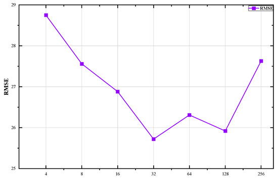
Figure 4.
The RMSE distribution with different batch size.
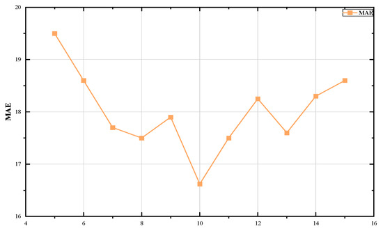
Figure 5.
The MAE distribution with different time step.
4.2. Baselines
In our experiments, we compared the predictive capabilities of the proposed AMGC-AT model and classical time-series models (ARIMA and HA), deep-learning-based models (LSTM, TCN and GCN), and existing advanced methods (MTGNN, AGCRN and STGCN).
ARIMA [2]: It is one of the most common statistical models used to predict time series. It represents a standard ARIMA model that uses historical data-fitting parameters to predict future metro passenger flow.
HA [1]: Historical average model. We use the average value of the last time step of three patterns to predict the value of the next time step.
LSTM [3]: LSTM was first introduced in transport in 2015. The long-term temporal characteristics of traffic flow sequences can be modeled by a time-series prediction model with three more gate control units than a typical RNN.
TCN [25]: A Convolution Neural Network with Dilation Causal Convolution for Sequence Modeling.
GCN [12]: Graph Convolution Neural Network is a prediction method for mining the spatial correlation of traffic flow. It should be noted that we performed GCN operations on all graphs in a comparative experiment.
MTGNN [21]: Multi-variable time-series prediction based on a graph neural network. MTGNN has designed a graphical learning module to learn spatial unidirectional correlations between variables. It proposes a convolution of graphs with mix-hop propagation and an extended starting layer for multi-variable time-series prediction.
STGCN [17]: spatial–temporal graph convolution network. STGCN is the fastest model to train in recent years, At the spatial feature level, the spatial dependencies between nodes are achieved using graph convolution neural networks, and sequences of traffic flows in terms of temporal characteristics are modelled using one-dimensional convolution.
AGCRN [26]: AGCRN proposes two adaptive learning modules to generate new adjacencies to better represent spatial correlations of nodes, enabling the use of GRU-based graph convolution networks to perform some multi-variable time-series prediction tasks without input of predefined adjacency matrices.
We compared our AMGC-AT model to the baseline and measured the performance of all methods using three widely used metrics: mean square root error (RMSE), mean absolute error (MAE), and weighted mean absolute percentage errors (WMAPE).
where denotes the total number of values that need to be predicted, is the predicted value and is the actual value.
4.3. Results and Analyses
We compared our AMGC-AT model to all baselines with three different prediction time intervals (10, 15, and 30 min). Table 3 shows a comparison of projections with ground realities. Our observations demonstrate that the proposed AMGC-AT model is superior to all baselines in all metrics regardless of time interval, demonstrating the robustness of our model. The bold data in Table 3 indicates the best results and the underlined data shows the second best.
Table 3.
Performance comparison of different methods on in-flow dataset.
4.3.1. Overall Comparison
- Traditional HA and ARIMA performed the worst in both the short and long term. The reason is that the two models capture only a limited temporal correlation and ignore some important but indispensable influences, such as the cyclical impact of urban residents’ daily travel patterns on subway traffic. In addition, important spatial and topological information about the subway network is missing.
- LSTM, TCN and GCN perform better than traditional models because they capture more temporal correlations and GCN captures more spatial correlations. However, the performance of the LSTM was significantly reduced in the long-term forecast. As can be observed, in most cases, complex deep-learning architectures (such as AGCRN, ST-GCN and MTGNN) yield more favorable results than single models. This is mainly because spatiotemporal features can be extracted from these models simultaneously.
- Notably, our self-attention based multi-graph approach has better performance in extracting joint spatiotemporal features compared to AGCRN, STGCN and MTGNN. Compared to STGCN, our model showed a significant increase in the accuracy of the predictions, because the AMGC-AT has two mechanisms of self-attention while the STGCN does not. For AGCRN and MTGNN, there are a number of differences compared to our proposed model. Firstly, AGCRN and MTGNN rely on their own adaptive graph-learning modules in order to learn the spatial correlations, while our proposed AMGC-AT relies on four different graph structures that use domain knowledge in order to learn spatial correlations, and our model is more direct and effective at learning spatial correlations. Secondly, MTGNN uses a mix-hop propagation graph solution, whereas STGCN, AGCRN, and our AMGC-AT all make use of spectral convolution, which is more suitable for node prediction on a metro network of this size. AGCRN also uses RNN to extract temporal features, which hurts the robustness of the model due to severe sample fluctuations and specific gradient explosions, while our AMGC-AT uses a more efficient gated convolution for extracting and outputting temporal features. In conclusion, compared to the most advanced models to date, only our model incorporates two self-attention mechanisms that are an integral part of AMGC-AT’s state-of-the-art performance. The effectiveness of the components of the AMGC-AT model will be analyzed and validated in the next chapter of the ablation experiment.
- In the case of RMSE, the significant improvements in three time intervals compared to the best (available) models were 16.74%, 14.47%, and 7.12%, respectively. The MAE improvement rates were 5.54%, 3.71% and 5.93%, respectively. Corresponding improvements in WMAPE were 12.52%, 5.2% and 8.53%, respectively.
- Figure 6 shows the distribution of RMSE errors for passenger inflow at 10-min granularity demonstrated using AMGC-AT and STGCN models. Yellow color indicates a relatively small error, and red color indicates a relatively large error. It is clear to see that the AMGC-AT model proposed in this paper can capture the variations of morning and evening peak passenger flow more efficiently and accurately to reduce the prediction error.
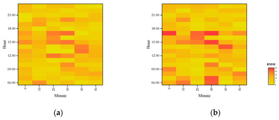 Figure 6. The RMSE errors distribution of inflow at 10-min granularity. (a) AMGC-AT; (b) STGCN.
4.3.2. Results Analysis
In order to test the model’s performance in the network-level prediction task, the prediction results for four stations were selected based on the degree distribution of the nodes in the metro station and compared to the STGCN network model. It should be noted that the experimental data used inflow passenger at ten-minute intervals.
The locations of the four metro stations are shown in Figure 7 below
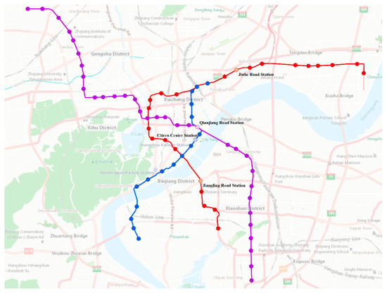
Figure 7.
Selected metro stations.
- Station 4: this is a Jianglin road station on Line 1, located in the Binjiang neighborhood of Hangzhou, surrounded by hospitals and schools, less than 500 m from the Binjiang government line.
- Station 18: Jiuhe road station on Line 1 is situated in the upper section of Hangzhou city. Today it is surrounded by farmhouses in both urban and rural areas. The surrounding areas will see more commercial and residential development.
- Station 46: Qianjiang Road Station on Line 2, with a degree value of 4 on the metro system, is situated in the upper city of Hangzhou and is a transfer station between Line 2 and Line 4 of the metro system. It is surrounded by many commercial and residential areas.
- Station 76: The Citizen Center Station on Line 4, with a degree value of 2 on the subway network, is located in the upper part of Hangzhou city. The station has eleven entrances and exits, and is surrounded by large complexes such as the Hangzhou Grand Theater, Hangzhou International Convention Center, and the Civic Center, among others.
Figure 8 shows that the AMGC-AT model and the STGCN model presented in this paper can accurately predict the flow of passengers on different routes, functions, and geographical locations. It should be noted that our model is most accurate at both peak and sub-peak times, and neither model can fit the fluctuations well at flat peak times, which we believe is related to the min–max normalization method causing the model to lose some sensitivity to numerical fluctuations at lower traffic volumes. However, the AMGC-AT model predictions were not significantly different from the actual values. We conclude that the prediction results demonstrate that our proposed model is reasonable and robust. This model will guide subway operators in making reasonable peak-period travel schedules and assist travelers in planning their trips.
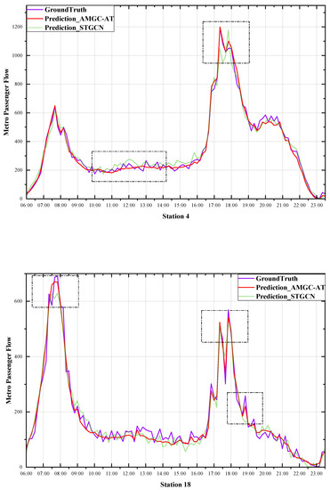
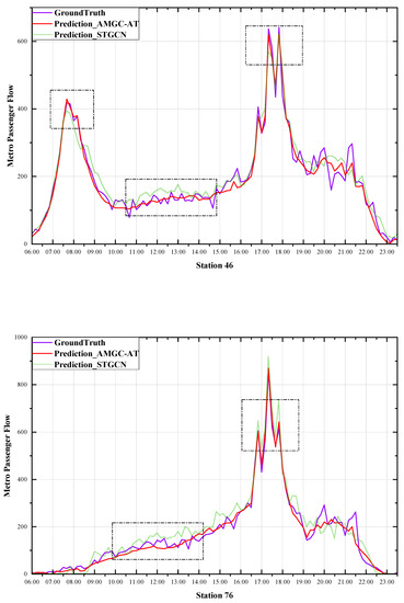
Figure 8.
Prediction results.
4.4. Ablation Study
To validate each component of the proposed AMGC-AT model, we performed further ablation studies. We compared our model to eight carefully designed variants. Although some changes were made, all variants have the same framework and parameter settings. Performance on the Hangzhou datasets is shown in Table 4.
Table 4.
Ablation study.
- AMGC-S: This variant eliminates the temporal self-attention mechanism and uses representations learned from spatial graphs directly to infer traffic flow.
- AMGC-T: This variant eliminates the spatial self-attention mechanism, while the other components remain the same, using only spatial features derived from multi-graph convolution to infer traffic flow.
- AGC-AT: This variant eliminates the convoluted components of Multi-graph and does not use predefined graph representations based on a priori knowledge constructs for feature extraction, leaving the components unchanged.
- AMG-AT: This variant removes the Multi-graph shared parameter section in the Multi-graph convolution component, which assumes that there is not sufficient correlation between predefined graph representations. The remaining components, including the spatiotemporal attention component and the causal convolution output component, remain the same.
- AGC1-AT: This variant removes the schematic representation of a station-based POI information construct in a multi-graph convolution component, leaving the rest of the component unchanged.
- AGC2-AT: This variant removes graphical representations of convoluted components based on station traffic volume similarity, leaving the rest of the component unchanged.
- AGC3-AT: This variant eliminates the schematic representation of the simrank-based convolution component, leaving the rest of the component unchanged.
- AMGC-AT1: This variant eliminates the periodic, short- and long-term division of traffic flow in the temporal and spatial self-attention component, with traffic flow information fed directly into the temporal and spatial self-attention component and the rest remaining the same.
- AMGC-AT2: This variant eliminates the short- and long-term division of traffic flows in the temporal and spatial self-attention segments; only the adjacent traffic flows are fed into the temporal and spatial self-attention segments, and the rest remain the same.
- AMGC-AT3: This variant eliminates the adjacent division of traffic flow in the temporal and spatial self-attention segments and only inputs traffic flow containing short-and long-term information into the temporal and spatial self-attention segments, leaving the remainder unchanged.
- AMGC-AT: The complete model presented in this paper.
As shown in Table 4, the experiment to verify the validity of each predefined graph of the multi-graph convolution component clearly demonstrates that the performance of the whole model decreases to varying degrees when removing any graph, which shows that the representation of the graph based on a priori knowledge is effective. Secondly, in the AMG-AT model, after removing the convoluted portion of the graph with shared parameters, the performance of the model decreased, suggesting that there is common information between graph representations based on different a priori knowledge that are not completely unrelated. Finally, the effects of periodic trends in traffic flow on model performance were verified by setting the AMGC-AT1, AMGC-AT2 and AMGC-AT3 models to compare the influence of adjacent and long-term trends in traffic flow on prediction accuracy. It is clear from Table 4 that the AMGC-AT model’s three modes of transportation—adjacent, daily and weekly—are reasonable.
5. Conclusions
AMGC-AT is proposed as a new traffic flow prediction model to address the problem whereby existing graph convolution-based traffic flow prediction methods cannot fully account for correlation variation characteristics in the metro cyberspace. By means of four types of diagrams based on the pre-conception of a priori knowledge, traffic flow data was characterized by long stretches of static space. The passenger flow was then split into three different time patterns based on analysis of the original passenger flow data, and dynamic spatial–temporal correlation of subway passenger flow was investigated through two mechanisms of self-attention. The AMGC-AT model presented in this paper is superior to the state-of-the-art baseline method in the publicly available Hangzhou Metro Real Traffic Dataset. Evidence for the validity and robustness of the AMGC-AT model comes from the passenger flow prediction results of subway stations with different geographic locations and regional functions, and the rationality of each component in the proposed model was tested through ablation experiments. AMGC-AT has disadvantages, however: (1) we did not consider external factors such as weather conditions and metro schedules; and (2) the flow of vacation passengers is more random and less regular, and vacation data were omitted from this research, so this limitation should be addressed in future studies. In the future, we will explore how to improve the model’s generalization and migratory learning capability, and transfer the model to other urban metro passenger flow prediction tasks. Finally, the availability of transportation big-data resources also varies from city to city, and for some cities data volume and variety are high; thus, the integration of heterogeneous transport data from multiple sources (e.g., text, images and video) is a potential hotspot in this field in the future. Migration learning and small-sample learning can be key solutions to this problem for cities with fewer data resources.
Author Contributions
Conceptualization, K.S.; methodology, F.W. and C.Z. (Chen Zhang); software, F.W.; validation, F.W. and C.Z. (Chen Zhang); formal analysis, F.W.; investigation, J.M; resources, K.S.; data curation, F.W. and J.M.; writing—original draft preparation, F.W. and C.Z. (Chen Zhang); writing—review and editing, F.W. and K.S.; visualization, J.M.; supervision, C.Z. (Changjiang Zheng); project administration, C.Z. (Changjiang Zheng); funding acquisition, C.Z. (Changjiang Zheng). All authors have read and agreed to the published version of the manuscript.
Funding
This work was supported in part by the Jiangsu Transportation Science and Technology Project (2021G09).
Institutional Review Board Statement
Not applicable.
Informed Consent Statement
Not applicable.
Data Availability Statement
The data used in this study are available in (https://tianchi.aliyun.com/competition/entrance/231708/introduction, accessed on 1 July 2022).
Acknowledgments
We gratefully wish to acknowledge the funding support from the Jiangsu Transportation Science and Technology Project Fund and the contribution of Yang Shen from Nanjing Communication Group.
Conflicts of Interest
The authors declare no conflict of interest.
References
- Smith, B.L.; Demetsky, M.J. Traffic flow forecasting: Comparison of modeling approaches. J. Transp. Eng. 1997, 123, 261–266. [Google Scholar] [CrossRef]
- Shekhar, S.; Williams, B.M. Adaptive seasonal time series models for forecasting short-term traffic flow. Transp. Res. Rec. J. Transp. Res. Board 2007, 2024, 116–125. [Google Scholar] [CrossRef]
- Ma, X.; Tao, Z.; Wang, Y.; Yu, H.; Wang, Y. Long short-term memory neural network for traffic speed prediction using Remote Microwave Sensor Data. Transp. Res. Part C Emerg. Technol. 2015, 54, 187–197. [Google Scholar] [CrossRef]
- Fu, R.; Zhang, Z.; Li, L. Using LSTM and GRU neural network methods for traffic flow prediction. In Proceedings of the 31st Youth Academic Annual Conference of Chinese Association of Automation (YAC 2016), Wuhan, China, 11–13 November 2016; pp. 324–328. [Google Scholar] [CrossRef]
- Jiang, W.; Zhang, L. Geospatial data to images: A deep-learning framework for traffic forecastin. Tsinghua Sci. Technol. 2019, 24, 52–64. [Google Scholar] [CrossRef]
- Ma, X.; Dai, Z.; He, Z.; Ma, J.; Wang, Y.; Wang, Y. Learning traffic as images: A deep convolutional neural network for large-scale transportation network speed prediction. Sensors 2017, 17, 818. [Google Scholar] [CrossRef] [PubMed]
- Zhao, Z.; Chen, W.; Wu, X.; Chen, P.C.Y.; Liu, J. LSTM network: A deep learning approach for short-term Traffic forecast. IET Intell. Transp. Syst. 2017, 11, 68–75. [Google Scholar] [CrossRef]
- Jiang, W.; Luo, J. Graph Neural Network for traffic forecasting: A survey. Expert Syst. Appl. 2022, 207, 117921. [Google Scholar] [CrossRef]
- Liu, Z.; Tan, H. Traffic prediction with Graph Neural Network: A survey. CICTP 2021, 2021, 467–474. [Google Scholar] [CrossRef]
- Scarselli, F.; Gori, M.; Tsoi, A.C.; Hagenbuchner, M.; Monfardini, G. The graph neural network model. IEEE Trans. Neural Netw. 2009, 20, 61–80. [Google Scholar] [CrossRef] [PubMed]
- Defferrard, M.; Bresson, X.; Vandergheynst, P. Convolutional neural networks on graphs with fast localized spectral filtering. arXiv 2017. [Google Scholar] [CrossRef]
- Kipf, T.N.; Welling, M. Semi-supervised classification with graph Convolutional Networks. arXiv 2017. [Google Scholar] [CrossRef]
- Atwood, J.; Towsley, D. Diffusion-Convolutional Neural Networks, Advances in Neural Information Processing Systems. 1970. Available online: https://papers.nips.cc/paper/2016/hash/390e982518a50e280d8e2b535462ec1f-Abstract.html (accessed on 12 December 2022).
- Gilmer, J.; Schoenholz, S.S.; Riley, P.F.; Vinyals, O.; Dahl, G.E. Message passing neural networks. In Machine Learning Meets Quantum Physics; Springer: Berlin/Heidelberg, Germany, 2020; pp. 199–214. [Google Scholar] [CrossRef]
- Hamilton, W.L.; Ying, R.; Leskovec, J. Inductive representation learning on large graphs. arXiv 2018. [Google Scholar] [CrossRef]
- Mattos, J.P.; Marcacini, R.M. Semi-supervised graph Attention Networks for Event Representation Learning. In Proceedings of the 2021 IEEE International Conference on Data Mining (ICDM), Auckland, New Zealand, 7–10 December 2021. [Google Scholar] [CrossRef]
- Yu, B.; Yin, H.; Zhu, Z. Spatio-temporal graph convolutional networks: A Deep Learning Framework for traffic forecasting. In Proceedings of the Twenty-Seventh International Joint Conference on Artificial Intelligence, Stockholm, Sweden, 13–19 July 2018. [Google Scholar] [CrossRef]
- Zhang, J.; Chen, F.; Guo, Y.; Li, X. Multi-graph Convolutional Network for short-term passenger flow forecasting in urban rail transit. IET Intell. Transp. Syst. 2020, 14, 1210–1217. [Google Scholar] [CrossRef]
- Zhao, L.; Song, Y.; Zhang, C.; Liu, Y.; Wang, P.; Lin, T.; Deng, M.; Li, H. T-GCN: A temporal graph convolutional network for traffic prediction. IEEE Trans. Intell. Transp. Syst. 2019, 21, 3848–3858. [Google Scholar] [CrossRef]
- Li, Y.; Yu, R.; Shahabi, C.; Liu, Y. Diffusion convolutional recurrent neural network: Data-driven traffic forecasting. In Proceedings of the 6th International Conference on Learning Representations, Vancouver, BC, Canada, 30 April–3 May 2018. [Google Scholar]
- Wu, Z.; Pan, S.; Long, G.; Jiang, J.; Chang, X.; Zhang, C. Connecting the dots: Multivariate time series forecasting with Graph Neural Networks. In Proceedings of the 26th ACM SIGKDD International Conference on Knowledge Discovery & Data Mining, Virtual Event, 6–10 July 2020. [Google Scholar] [CrossRef]
- Geng, X.; Li, Y.; Wang, L.; Zhang, L.; Yang, Q.; Ye, J.; Liu, Y. Spatiotemporal multi-graph convolution network for ride-hailing demand forecasting. Proc. AAAI Conf. Artif. Intell. 2019, 33, 3656–3663. [Google Scholar] [CrossRef]
- Li, D.; Lasenby, J. Spatiotemporal attention-based graph convolution network for segment-level traffic prediction. IEEE Trans. Intell. Transp. Syst. 2022, 23, 8337–8345. [Google Scholar] [CrossRef]
- Qiao, S.; Li, T.; Li, H.; Zhu, Y.; Peng, J.; Qiu, J. SimRank: A page rank approach based on similarity measure. In Proceedings of the 2010 IEEE International Conference on Intelligent Systems and Knowledge Engineering, Hangzhou, China, 15–16 November 2010. [Google Scholar] [CrossRef]
- Bai, S.; Kolter, J.Z.; Koltun, V. An empirical evaluation of generic convolutional and recurrent networks for sequence modeling. arXiv 2018. [Google Scholar] [CrossRef]
- Bai, L.; Yao, L.; Li, C.; Wang, X.; Wang, C. Adaptive graph convolutional recurrent network for traffic forecasting. In Proceedings of the 34th International Conference on Neural Information Processing Systems, Online, 6–12 December 2020. [Google Scholar] [CrossRef]


Disclaimer/Publisher’s Note: The statements, opinions and data contained in all publications are solely those of the individual author(s) and contributor(s) and not of MDPI and/or the editor(s). MDPI and/or the editor(s) disclaim responsibility for any injury to people or property resulting from any ideas, methods, instructions or products referred to in the content. |
© 2023 by the authors. Licensee MDPI, Basel, Switzerland. This article is an open access article distributed under the terms and conditions of the Creative Commons Attribution (CC BY) license (https://creativecommons.org/licenses/by/4.0/).