

Binary and Multi-Class Malware Threads Classification


Abstract
1. Introduction
- To present an effective malware detection and classification method, SFTA and Gabor are extracted as distinctive feature vectors.
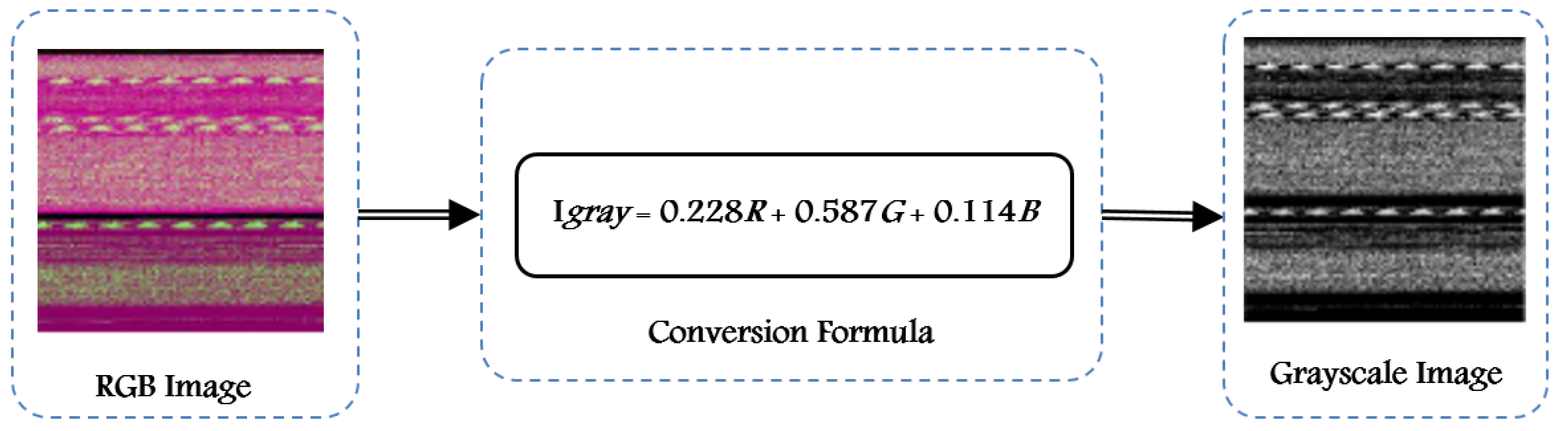
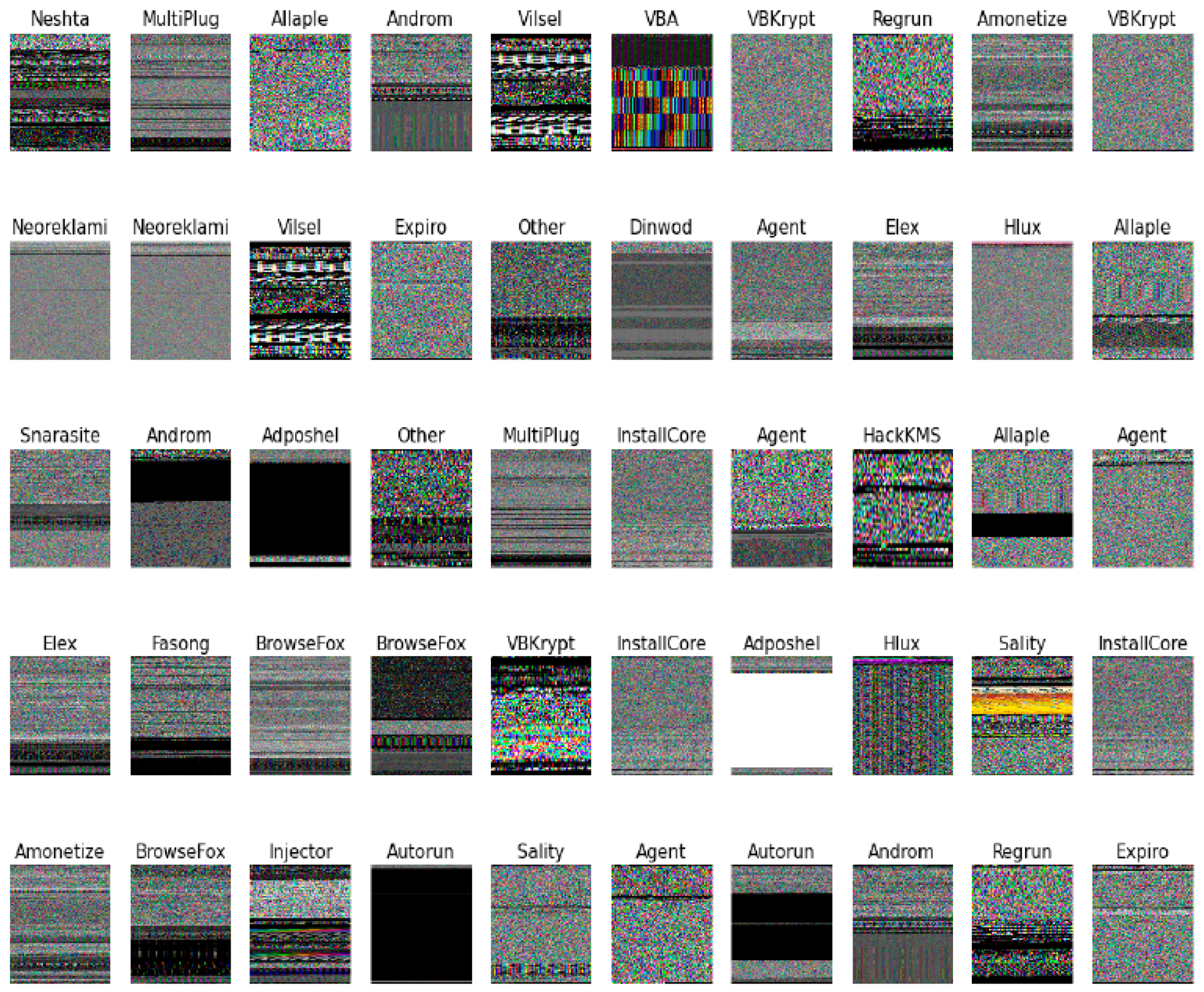
- The usage of a malware visualization method that transforms binary files to 8 bit vectors for create grayscale graphics.
- SFTA-GDA minimizes processing times and enhances overall detection/classification accuracy through texture features.
- Experiment findings demonstrate that the proposed technique can accurately classify malware families.
- Experimental results show that our proposed method can classify malware families with a low rate of false positives and false negatives.
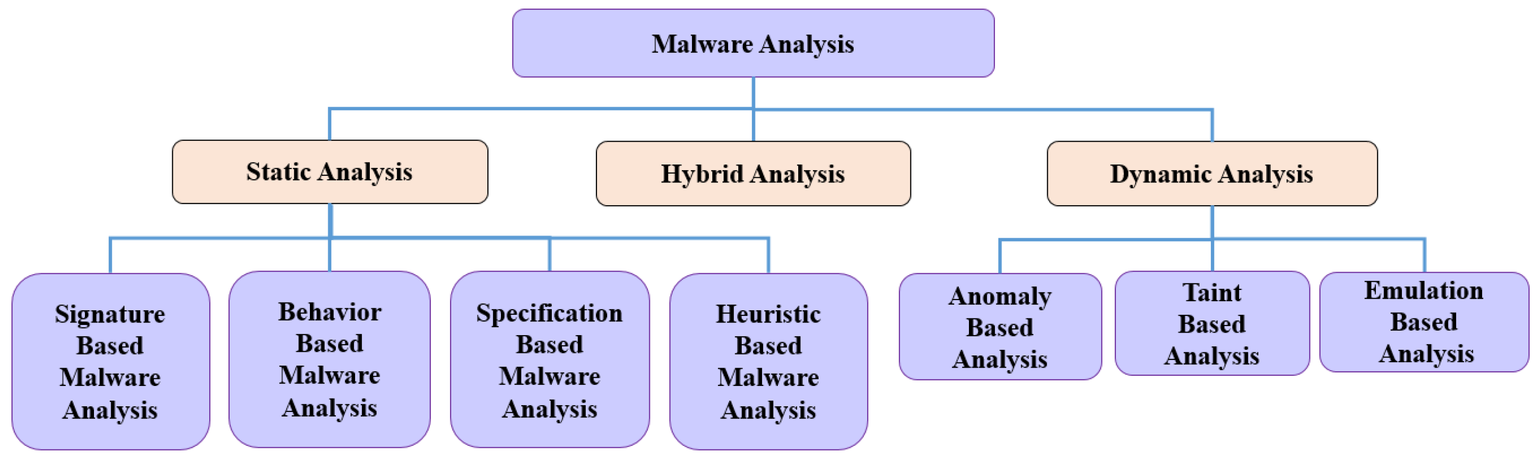
2. Related Works
3. Multiple Features
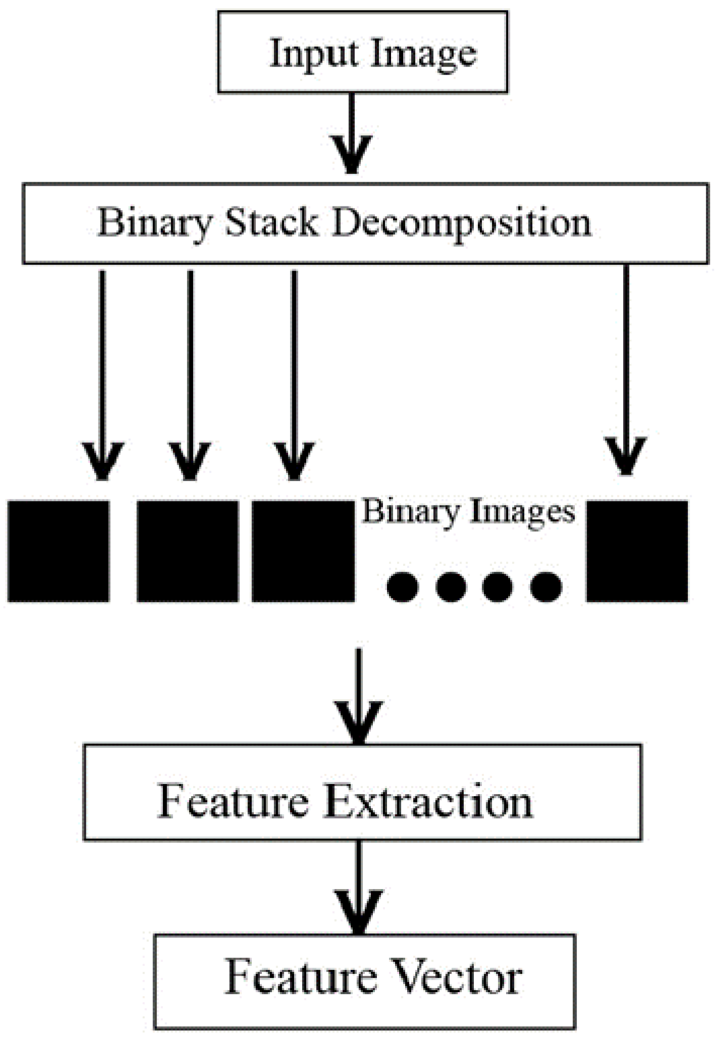
3.1. Segmentation-Based Fractal Texture Analysis (SFTA)
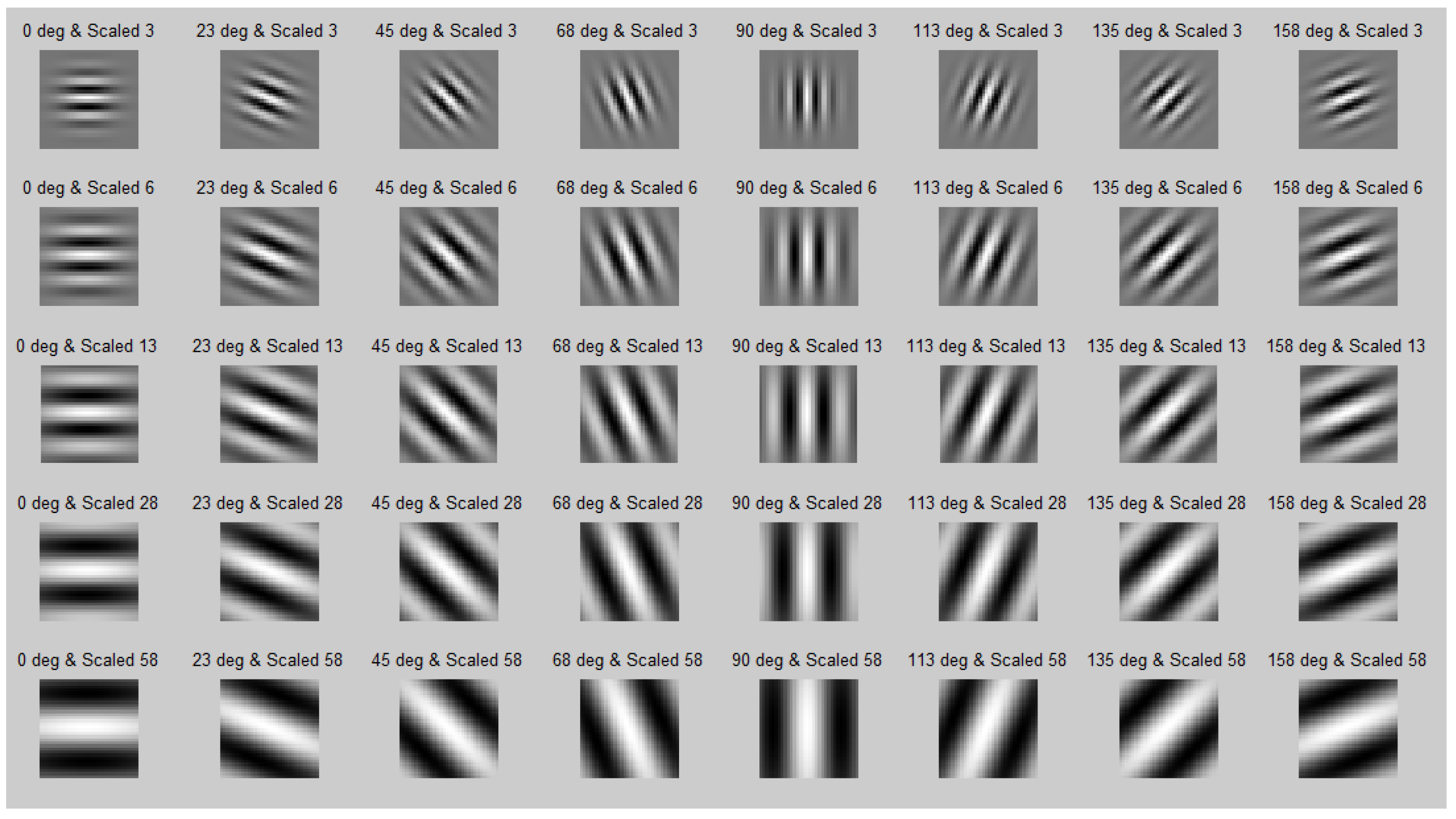
3.2. Gabor Features
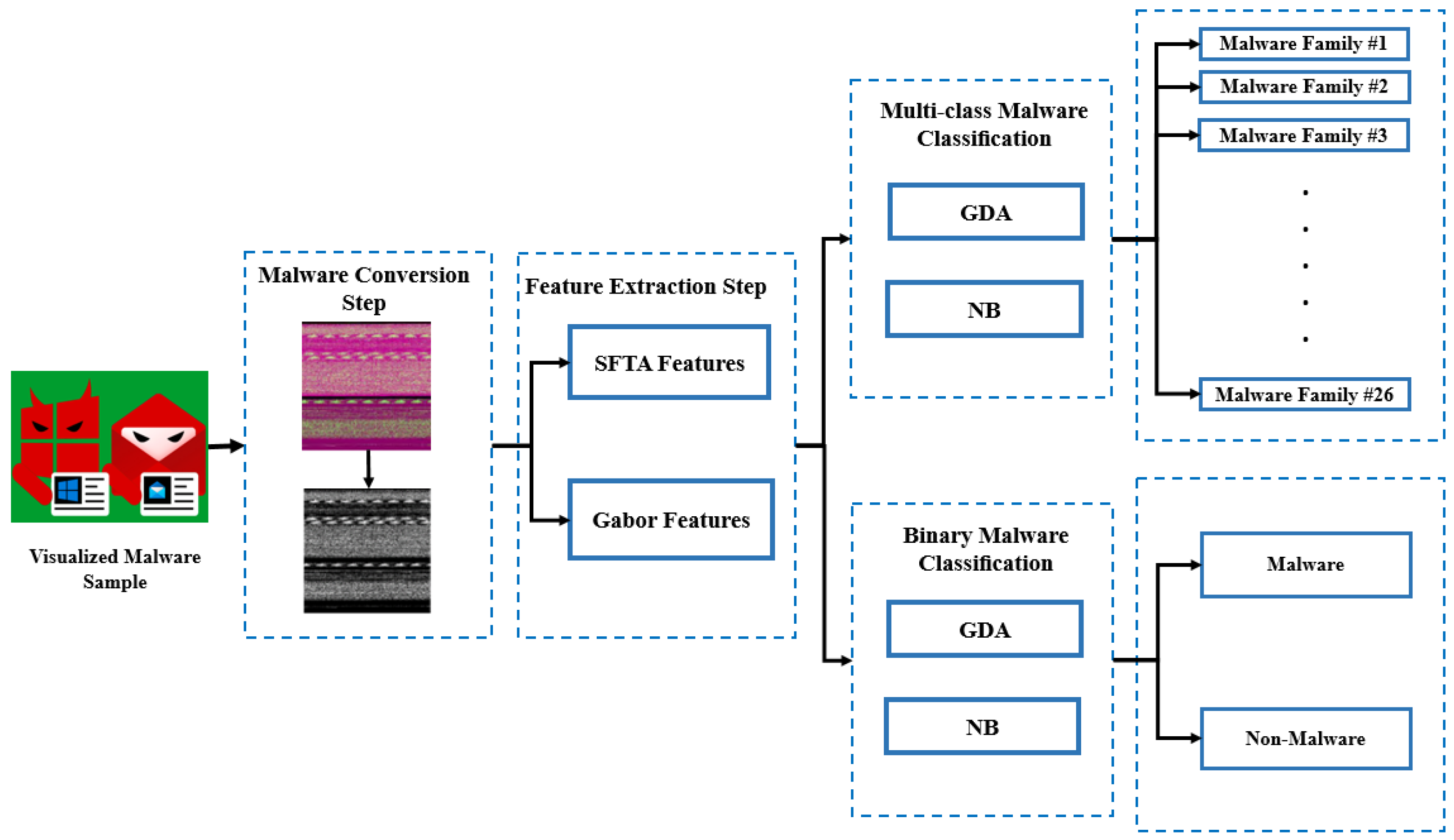
4. The Proposed Methods
| Algorithm 1: Proposed MC_based GDA and NB Classifier. |
| Input: RGB Malware Image. Output: Non-Malware/Malware Image. Begin For 1: Use the “Imread ()” function to read each image; 2: Convert the RGB image to the gray-scale image using Matlab function such as “rgb2gray ( )”; 3: Then, the SFTA features {Sftaf1, Sftaf2, Sftaf3, Sftaf4,… Sftaf21} are extracted to obtain 1 × 21-dimension feature vector; 4: Extract the Gabor features vector:
End |
- Step 1: Malware Conversion
- Step 2: Feature Extraction
- Step 2.1: SFTA Features Extraction
| Algorithm 2: Compute SFTA textures features. |
| Input: Visualized Malware Image. Output: 1 × 21 features vector dimension.
|
- Step 2.2: Gabor Features Extraction
| Algorithm 3: Compute Gabor textures features. |
| Input: Visualized Malware Image. Output: 1 × 12 features vector dimension.
|
- Step 3: Classification
- Step 3.1: Naive Bayes (NB) Classifier
- Step 3.2: Gaussian discriminant analysis (GDA) Classifier
5. Results and Discussion
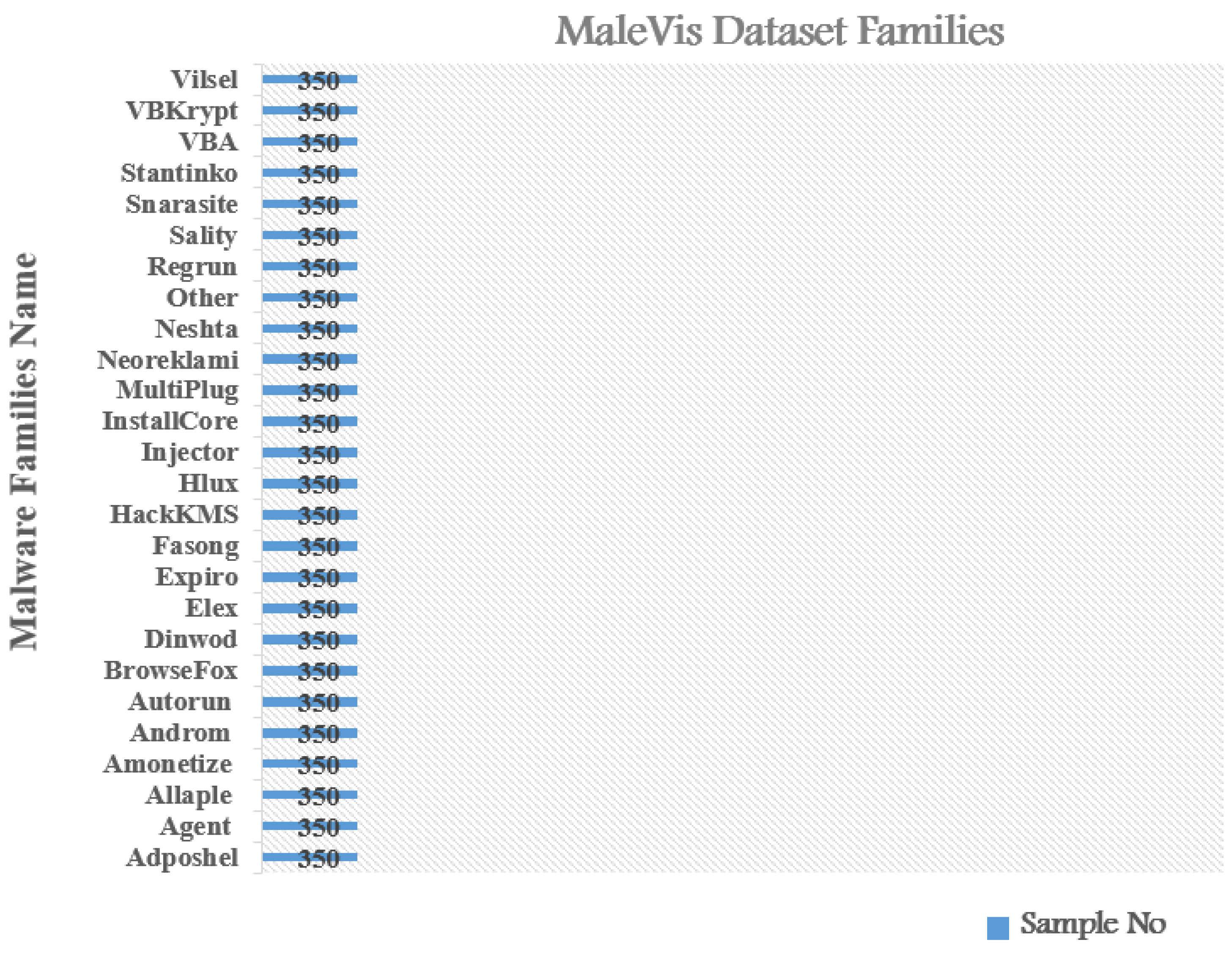
5.1. Datasets
5.2. Performance Evaluation Metric
- The term “TP” (True Positive) refers to the variety of malware types that may be considered to be positive.
- The term “TN” (True Negative) refers to the variety of malware types that may be considered to be negative.
- The term “FP” (False Positive) refers to the variety of malware types that may be considered to be negative and positive.
- The term “FN” (False Negative) refers to the variety of malware types that may be considered to be negative and positive.
5.3. Evaluation Results
5.3.1. Binary Malware Classification Results
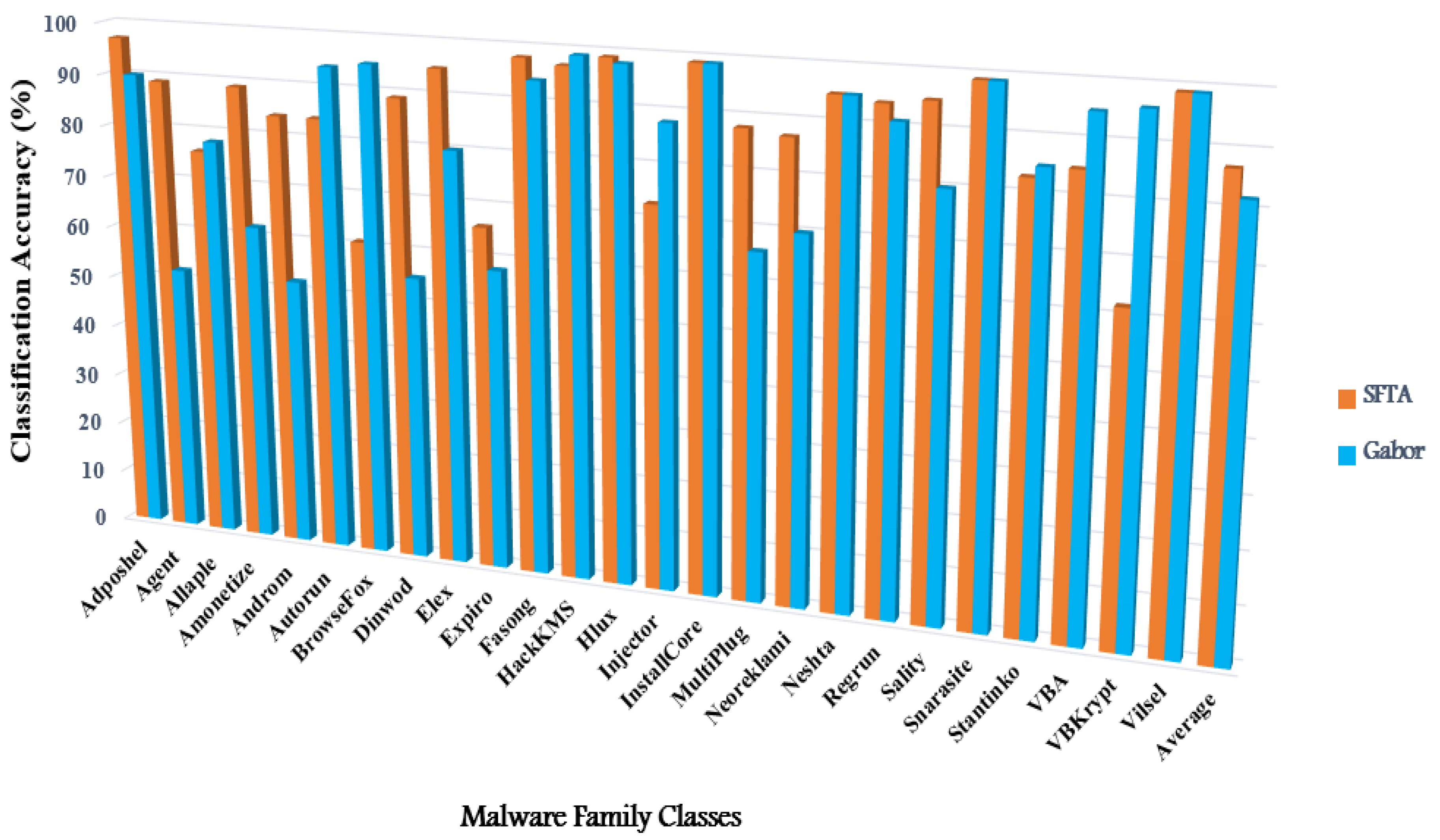
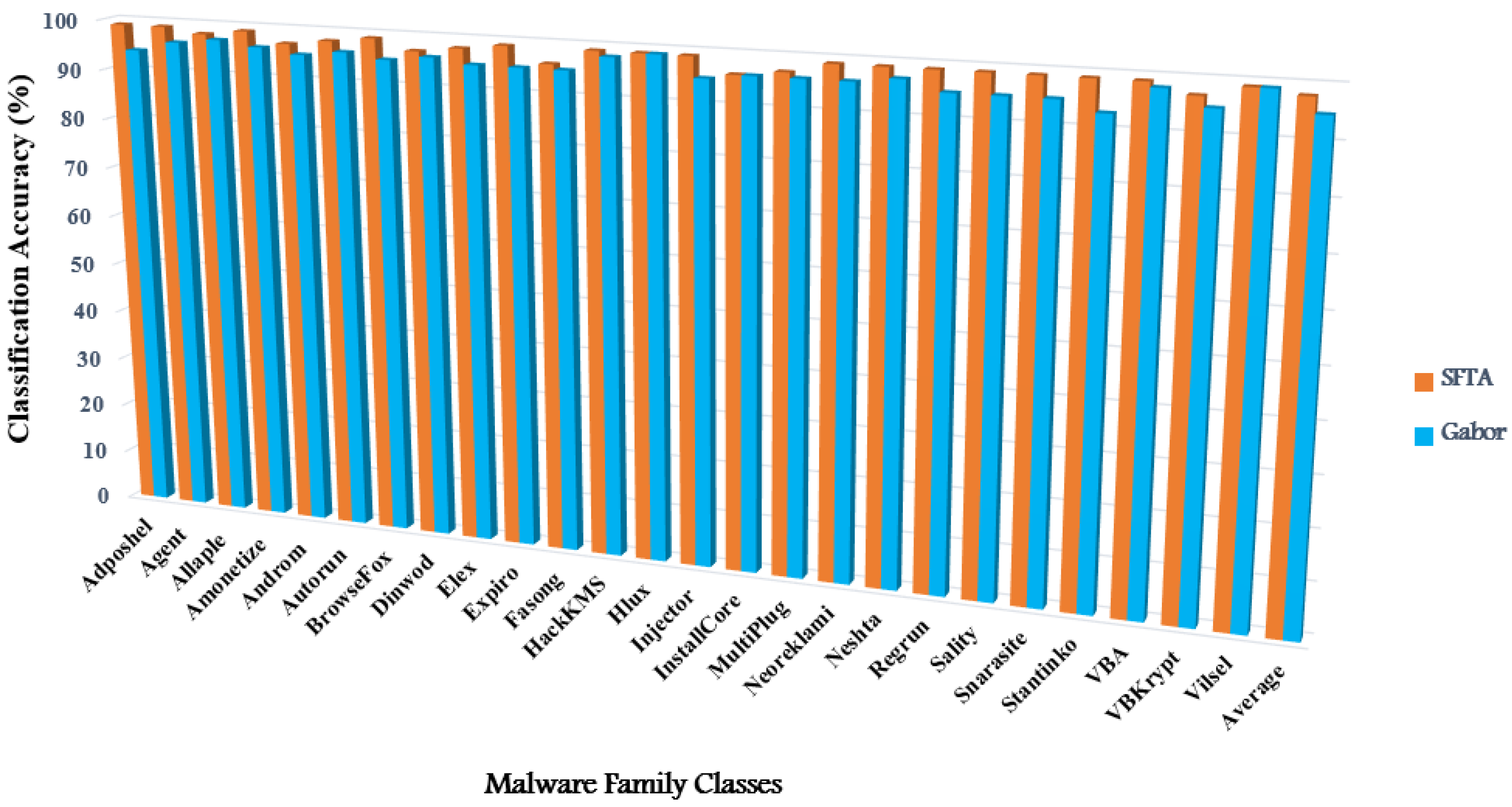
5.3.2. Multi-Class Malware Classification Results
5.4. Existing Methods Comparison Results
6. Conclusions
Author Contributions
Funding
Institutional Review Board Statement
Informed Consent Statement
Data Availability Statement
Conflicts of Interest
References
- Poudyal, S.; Akhtar, Z.; Dasgupta, D.; Gupta, K.D. Malware analytics: Review of data mining, machine learning and big data perspectives. In Proceedings of the 2019 IEEE Symposium Series on Computational Intelligence (SSCI), Xiamen, China, 6–9 December 2019; pp. 649–656. [Google Scholar]
- Hemalatha, J.; Roseline, S.A.; Geetha, S.; Kadry, S.; Damaševičius, R. An efficient densenet-based deep learning model for malware detection. Entropy 2021, 23, 344. [Google Scholar] [CrossRef] [PubMed]
- O’Brien, D. Internet Security Threat Report-Ransomware 2017. Symantec 2017, 11, 203–214. [Google Scholar]
- Makandar, A.; Patrot, A. Malware class recognition using image processing techniques. In Proceedings of the 2017 International Conference on Data Management, Analytics and Innovation (ICDMAI), Pune, India, 24–26 February 2017; pp. 76–80. [Google Scholar]
- Verma, V.; Muttoo, S.K.; Singh, V.B. Multiclass malware classification via first-and second-order texture statistics. Comput. Secur. 2020, 97, 101895. [Google Scholar] [CrossRef]
- Aslan, Ö. Performance comparison of static malware analysis tools versus antivirus scanners to detect malware. In Proceedings of the International Multidisciplinary Studies Congress (IMSC), Solin, Croatia, 20–21 April 2017. [Google Scholar]
- Naeem, H.; Guo, B.; Naeem, M.R.; Ullah, F.; Aldabbas, H.; Javed, M.S. Identification of malicious code variants based on image visualization. Comput. Electr. Eng. 2019, 76, 225–237. [Google Scholar] [CrossRef]
- Bayer, U.; Moser, A.; Kruegel, C.; Kirda, E. Dynamic analysis of malicious code. J. Comput. Virol. 2006, 2, 67–77. [Google Scholar] [CrossRef]
- Nataraj, L.; Karthikeyan, S.; Jacob, G.; Manjunath, B.S. Malware images: Visualization and automatic classification. In Proceedings of the 8th International Symposium on Visualization for Cyber Security, Pittsburgh PA, USA, 20 July 2011; pp. 1–7. [Google Scholar]
- Nataraj, L.; Yegneswaran, V.; Porras, P.; Zhang, J. A comparative assessment of malware classification using binary texture analysis and dynamic analysis. In Proceedings of the 4th ACM Workshop on Security and Artificial Intelligence, Chicago, IL, USA; 2011; pp. 21–30. [Google Scholar]
- Torralba, A.; Murphy, K.P.; Freeman, W.T.; Rubin, M.A. Context-based vision system for place and object recognition. In Proceedings of the Ninth IEEE International Conference on Computer Vision, Nice, France, 13–16 October 2003; Volume 2, p. 273. [Google Scholar]
- Oliva, A.; Torralba, A. Modeling the shape of the scene: A holistic representation of the spatial envelope. Int. J. Comput. Vis. 2001, 42, 145–175. [Google Scholar] [CrossRef]
- Han, K.; Kang, B.; Im, E.G. Malware analysis using visualized image matrices. Sci. World J. 2014, 2014, 132713. [Google Scholar] [CrossRef]
- Gandotra, E.; Bansal, D.; Sofat, S. Integrated framework for classification of malwares. In Proceedings of the 7th International Conference on Security of Information and Networks, Scotland, UK, 9–11 September 2014; pp. 417–422. [Google Scholar]
- Han, K.S.; Lim, J.H.; Kang, B.; Im, E.G. Malware analysis using visualized images and entropy graphs. Int. J. Inf. Secur. 2015, 14, 1–14. [Google Scholar] [CrossRef]
- Vinayakumar, R.; Alazab, M.; Soman, K.P.; Poornachandran, P.; Venkatraman, S. Robust intelligent malware detection using deep learning. IEEE Access 2019, 7, 46717–46738. [Google Scholar] [CrossRef]
- Li, F.-Q.; Wang, S.-L.; Liew, A.W.-C.; Ding, W.; Liu, G.-S. Large-Scale Malicious Software Classification With Fuzzified Features and Boosted Fuzzy Random Forest. IEEE Trans. Fuzzy Syst. 2020, 29, 3205–3218. [Google Scholar] [CrossRef]
- Kong, D.; Yan, G. Discriminant malware distance learning on structural information for automated malware classification. In Proceedings of the 19th ACM SIGKDD International Conference on Knowledge Discovery and Data Mining, Chicago, IL, USA, 11–14 August 2013; pp. 1357–1365. [Google Scholar]
- Kosmidis, K.; Kalloniatis, C. Machine learning and images for malware detection and classification. In Proceedings of the 21st Pan-Hellenic Conference on Informatics, Larissa, Greece, 28–30 September 2017; pp. 1–6. [Google Scholar]
- Xiaofang, B.; Li, C.; Weihua, H.; Qu, W. Malware variant detection using similarity search over content fingerprint. In Proceedings of the 26th Chinese Control and Decision Conference (2014 CCDC), Changsha, China, 31 May–2 June 2014; pp. 5334–5339. [Google Scholar]
- Liu, Y.; Lai, Y.-K.; Wang, Z.-H.; Yan, H.-B. A new learning approach to malware classification using discriminative feature extraction. IEEE Access 2019, 7, 13015–13023. [Google Scholar] [CrossRef]
- Fu, J.; Xue, J.; Wang, Y.; Liu, Z.; Shan, C. Malware visualization for fine-grained classification. IEEE Access 2018, 6, 14510–14523. [Google Scholar] [CrossRef]
- Liu, L.; Wang, B. Malware classification using gray-scale images and ensemble learning. In Proceedings of the 2016 3rd International Conference on Systems and Informatics (ICSAI), Shanghai, China, 19–21 November 2016; pp. 1018–1022. [Google Scholar]
- Bozkir, A.S.; Tahillioglu, E.; Aydos, M.; Kara, I. Catch them alive: A malware detection approach through memory forensics, manifold learning and computer vision. Comput. Secur. 2021, 103, 102166. [Google Scholar] [CrossRef]
- Costa, A.F.; Humpire-Mamani, G.; Traina, A.J.M. An efficient algorithm for fractal analysis of textures. In Proceedings of the 2012 25th SIBGRAPI Conference on Graphics, Patterns and Images, Ouro Preto, Brazil, 22–25 August 2012; pp. 39–46. [Google Scholar]
- Hammad, B.T.; Ahmed, I.T.; Jamil, N. A Steganalysis Classification Algorithm Based on Distinctive Texture Features. Symmetry 2022, 14, 236. [Google Scholar] [CrossRef]
- Daugman, J.G. Uncertainty relation for resolution in space, spatial frequency, and orientation optimized by two-dimensional visual cortical filters. JOSA A 1985, 2, 1160–1169. [Google Scholar] [CrossRef]
- Song, X.; Liu, F.; Zhang, Z.; Yang, C.; Luo, X.; Chen, L. 2D Gabor filters-based steganalysis of content-adaptive JPEG steganography. Multimed. Tools Appl. 2017, 76, 26391–26419. [Google Scholar] [CrossRef]
- Zheng, D.; Zhao, Y.; Wang, J. Features extraction using a Gabor filter family. In Proceedings of the sixth Lasted International Conference, Signal and Image Processing, Hawaii, HI, USA, 23–25 August 2004. [Google Scholar]
- SwagotaBera, D.; Sharma, M.; Singh, B. Feature extraction and analysis using Gabor filter and higher order statistics for the JPEG steganography. Int. J. Appl. Eng. Res. 2018, 13, 2945–2954. [Google Scholar]
- Ahmed, I.T.; Hammad, B.T.; Jamil, N. Common Gabor Features for Image Watermarking Identification. Appl. Sci. 2021, 11, 8308. [Google Scholar] [CrossRef]
- Kamarainen, J.-K. Gabor features in image analysis. In Proceedings of the 2012 3rd International Conference on Image Processing Theory, Tools and Applications (IPTA), Istanbul, Turkey, 15–18 October 2012; pp. 13–14. [Google Scholar]
- Lowd, D.; Domingos, P. Naive Bayes models for probability estimation. In Proceedings of the 22nd International Conference on Machine Learning, Bonn, Germany, 7–11 August 2005; pp. 529–536. [Google Scholar]
- Sharifi, K.; Leon-Garcia, A. Estimation of shape parameter for generalized Gaussian distributions in subband decompositions of video. IEEE Trans. Circuits Syst. Video Technol. 1995, 5, 52–56. [Google Scholar] [CrossRef]
- Bozkir, A.S.; Cankaya, A.O.; Aydos, M. Utilization and comparision of convolutional neural networks in malware recognition. In Proceedings of the 2019 27th Signal Processing and Communications Applications Conference (SIU), Sivas, Turkey, 24–26 April 2019; pp. 1–4. [Google Scholar]
- Patil, S.; Varadarajan, V.; Walimbe, D.; Gulechha, S.; Shenoy, S.; Raina, A.; Kotecha, K. Improving the Robustness of AI-Based Malware Detection Using Adversarial Machine Learning. Algorithms 2021, 14, 297. [Google Scholar] [CrossRef]
- Hammad, B.T.; Jamil, N.; Ahmed, I.T.; Zain, Z.M.; Basheer, S. Robust Malware Family Classification Using Effective Features and Classifiers. Appl. Sci. 2022, 12, 7877. [Google Scholar] [CrossRef]
- Ahmed, I.T.; Hammad, B.T.; Jamil, N. A comparative analysis of image copy-move forgery detection algorithms based on hand and machine-crafted features. Indones. J. Electr. Eng. Comput. Sci. 2021, 22, 1177–1190. [Google Scholar]
- Ahmed, I.T.; Hammad, B.T.; Jamil, N. Image Copy-Move Forgery Detection Algorithms Based on Spatial Feature Domain. In Proceedings of the 2021 IEEE 17th International Colloquium on Signal Processing & Its Applications (CSPA), Langkawi, Malaysia, 5–6 March 2021; pp. 92–96. [Google Scholar]
- Ahmed, I.T.; Der, C.S.; Jamil, N.; Mohamed, M.A. Improve of contrast-distorted image quality assessment based on convolutional neural networks. Int. J. Electr. Comput. Eng. 2019, 9, 5604–5614. [Google Scholar] [CrossRef]
- Kang, H.; Jang, J.; Mohaisen, A.; Kim, H.K. Detecting and classifying android malware using static analysis along with creator information. Int. J. Distrib. Sens. Netw. 2015, 11, 479174. [Google Scholar] [CrossRef]
- Makandar, A.; Patrot, A. Wavelet statistical feature based malware class recognition and classification using supervised learning classifier. Orient. J. Comput. Sci. Technol. 2017, 10, 400–406. [Google Scholar] [CrossRef]
- Hashemi, H.; Hamzeh, A. Visual malware detection using local malicious pattern. J. Comput. Virol. Hacking Tech. 2019, 15, 1–14. [Google Scholar] [CrossRef]
- Nisa, M.; Shah, J.H.; Kanwal, S.; Raza, M.; Khan, M.A.; Damaševičius, R.; Blažauskas, T. Hybrid malware classification method using segmentation-based fractal texture analysis and deep convolution neural network features. Appl. Sci. 2020, 10, 4966. [Google Scholar] [CrossRef]
- Mohammed, T.M.; Nataraj, L.; Chikkagoudar, S.; Chandrasekaran, S.; Manjunath, B.S. Malware detection using frequency domain-based image visualization and deep learning. arXiv 2021, arXiv:2101.10578. [Google Scholar]


| Hardware | Properties |
|---|---|
| PC | HP laptop |
| Operating system | Microsoft Windows 10 64-bit (OS) |
| RAM | 8 GB |
| Processor | Intel(R) Core(TM) i7-6500U CPU @ 2.50 GHz 2.60 GHz |
| Software | MATLAB version R2020a |
| Graphics Card | Intel® HD Graphics 520 (NVIDIA GTX 950M) |
| Class ID | Family | Details | |
|---|---|---|---|
| Malware Category | Sample No. | ||
| #1 | Adposhel | Adware | 350 |
| #2 | Agent | Trojan | 350 |
| #3 | Allaple | Worm | 350 |
| #4 | Amonetize | Adware | 350 |
| #5 | Androm | Backdoor | 350 |
| #6 | Autorun | Worm | 350 |
| #7 | BrowseFox | Adware | 350 |
| #8 | Dinwod | Trojan | 350 |
| #9 | Elex | Trojan | 350 |
| #10 | Expiro | Virus | 350 |
| #11 | Fasong | Trojan | 350 |
| #12 | HackKMS | Riskware | 350 |
| #13 | Hlux | Worm | 350 |
| #14 | Injector | Trojan | 350 |
| #15 | InstallCore | Adware | 350 |
| #16 | MultiPlug | Adware | 350 |
| #17 | Neoreklami | Adware | 350 |
| #18 | Neshta | Virus | 350 |
| #19 | Other | - | 350 |
| #20 | Regrun | Trojan | 350 |
| #21 | Sality | Virus | 350 |
| #22 | Snarasite | Trojan | 350 |
| #23 | Stantinko | Trojan | 350 |
| #24 | VBA | Macro Malwares | 350 |
| #25 | VBKrypt | Trojan | 350 |
| #26 | Vilsel | Trojan | 350 |
| Total | - | 9100 | |
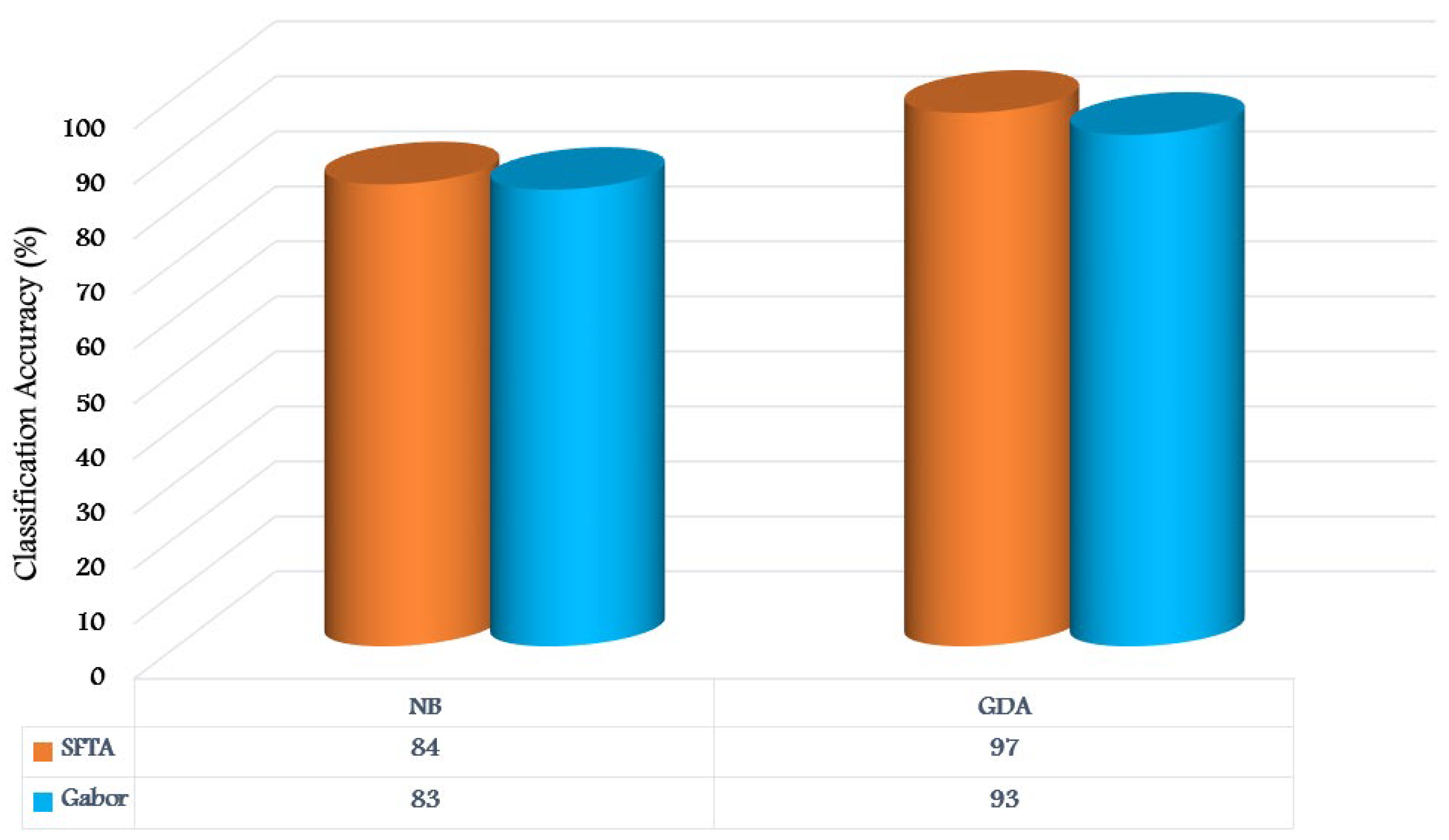
| Classifier | Detection Accuracy (%) | |
|---|---|---|
| SFTA Feature | Gabor Feature | |
| NB | 84 | 83 |
| GDA | 97 | 93 |
| Class ID | Family Name | Classification Accuracy (%) | |||
|---|---|---|---|---|---|
| Naive Classifier | GDA Classifier | ||||
| SFTA Feature | Gabor Feature | SFTA Feature | Gabor Feature | ||
| #1 | Adposhel | 97 | 90 | 99 | 94 |
| #2 | Agent | 89 | 52 | 99 | 96 |
| #3 | Allaple | 76 | 78 | 98 | 97 |
| #4 | Amonetize | 89 | 62 | 99 | 96 |
| #5 | Androm | 84 | 52 | 97 | 95 |
| #6 | Autorun | 84 | 94 | 98 | 96 |
| #7 | BrowseFox | 61 | 95 | 99 | 95 |
| #8 | Dinwod | 89 | 55 | 97 | 96 |
| #9 | Elex | 95 | 80 | 98 | 95 |
| #10 | Expiro | 66 | 58 | 99 | 95 |
| #11 | Fasong | 98 | 94 | 96 | 95 |
| #12 | HackKMS | 97 | 99 | 99 | 98 |
| #13 | Hlux | 99 | 98 | 99 | 99 |
| #14 | Injector | 73 | 88 | 99 | 95 |
| #15 | InstallCore | 99 | 99 | 96 | 96 |
| #16 | MultiPlug | 88 | 66 | 97 | 96 |
| #17 | Neoreklami | 87 | 70 | 99 | 96 |
| #18 | Neshta | 95 | 95 | 99 | 97 |
| #19 | Regrun | 94 | 91 | 99 | 95 |
| #20 | Sality | 95 | 80 | 99 | 95 |
| #21 | Snarasite | 99 | 99 | 99 | 95 |
| #22 | Stantinko | 83 | 85 | 99 | 93 |
| #23 | VBA | 85 | 95 | 99 | 98 |
| #24 | VBKrypt | 62 | 96 | 97 | 95 |
| #25 | Vilsel | 99 | 99 | 99 | 99 |
| Average | 87 | 82% | 98% | 95% | |
| Methods | Data Analysis | Feature Kind | Classifier Kind | Dataset | Accuracy (%) |
|---|---|---|---|---|---|
| Kang et al. [41] | Static | creator information | SVM | Malware | 90 |
| Makandar et al. [4] | Static | Gabor GIST DWT | KNN | Malimg | 98 |
| Aziz et al. [42] | Static | DWT | SVM | Mahenhuer | 92 |
| Hashemi et al. [43] | Static | LBP | KNN | Malimg | 91 |
| Liu et al. [21] | Static | GIST | RF | Malimg | 91 |
| Nisa et al. [44] | Static | SFTA | SVM | Malimg | 95 |
| Nisa et al. [44] | Static | Fused SFTA and DNN features | cubic SVM | Malimg | 99 |
| Patil et al. [36] | Static | - | Random f | MaleVis | 93 |
| Mohammed et al. [45] | Static | DCT | CNN | MaleVis | 96 |
| Proposed (SFTA-GDA) | Static | SFTA | GDA | MaleVis | 98 |
Publisher’s Note: MDPI stays neutral with regard to jurisdictional claims in published maps and institutional affiliations. |
© 2022 by the authors. Licensee MDPI, Basel, Switzerland. This article is an open access article distributed under the terms and conditions of the Creative Commons Attribution (CC BY) license (https://creativecommons.org/licenses/by/4.0/).
Share and Cite
Ahmed, I.T.; Jamil, N.; Din, M.M.; Hammad, B.T. Binary and Multi-Class Malware Threads Classification. Appl. Sci. 2022, 12, 12528. https://doi.org/10.3390/app122412528
Ahmed IT, Jamil N, Din MM, Hammad BT. Binary and Multi-Class Malware Threads Classification. Applied Sciences. 2022; 12(24):12528. https://doi.org/10.3390/app122412528
Chicago/Turabian StyleAhmed, Ismail Taha, Norziana Jamil, Marina Md. Din, and Baraa Tareq Hammad. 2022. "Binary and Multi-Class Malware Threads Classification" Applied Sciences 12, no. 24: 12528. https://doi.org/10.3390/app122412528
APA StyleAhmed, I. T., Jamil, N., Din, M. M., & Hammad, B. T. (2022). Binary and Multi-Class Malware Threads Classification. Applied Sciences, 12(24), 12528. https://doi.org/10.3390/app122412528