A Simple Method to Estimate Weed Control Threshold by Using RGB Images from Drones

Abstract

The estimation of the infestation level in a field and the consequent determination of the economic threshold is a basic requisite to rationalize post-emergence weeding. In this study, a simple and inexpensive procedure to determine the economic threshold based on weed cover is proposed. By using high-resolution RGB images captured by a low-cost drone, a free downloadable app for image processing and common spreadsheet software to perform the model parametrization, two different methods have been tested. The first method was based on the joint estimation of the two parameters involved in weed cover calculation, whereas the second method required the availability of further images for the separate estimation of the first parameter. The reliability of the two methods has been evaluated through the comparison with observed data and the goodness of fit in parameter calibration has been verified by calculating appropriate quality indices. The results showed an acceptable estimation of the weed cover value for the second method with respect to observed data (0.24 vs. 0.17 m² and 0.17 vs. 0.14 m², by processing images captured at 10 and 20 m, respectively), whereas the estimations obtained with the first method were disappointing (0.35 vs. 0.17 m² and 0.33 vs. 0.14 m², by processing images captured at 10 and 20 m, respectively).

1. Introduction

Never before has the use of pesticides, and especially herbicides, been at the centre of a global debate that has involved multifaceted issues making this matter increasingly complex [1,2]. Although the evidence of the negative effects on health and the environment caused by the use of herbicides has been underlined by many authors [3,4], we have recorded a significant increase in applied quantities over the last decades [5,6], confirming, for the time being, the reliance of agriculture on their use. Despite the increasing availability of herbicides that can be used at low doses and the efforts made by the EU to regulate this matter [7], in 2020, almost 346,000 tonnes of herbicides were sold in Europe [8].

Many recent research activities have been devoted to reducing herbicide consumption in order to support the transition from conventional to agroecological cropping systems [9,10]. According to [11], the first step in this process is to reduce the external-farm input use by making their use more efficient. For the last six decades, integrated pest management (IPM) has been the main response provided by researchers to improve crop protection strategies, and although its adoption has not proved to be as effective as hoped [12], the evaluation of weed infestation levels and the establishment of the action threshold is one of the pillars of integrated weed management (IWM) [13,14]. Nevertheless, the weed control threshold has been questioned as a problem-solving concept.

The reasons are numerous [15,16]: (i) the costs and difficulties of determining the real incidence of weed presence in relation to their random distribution in fields; (ii) the unreliability of models used to estimate yield losses because of their inability to consider the different competition level attributable to each weed species and the effects of other factors influencing crop production (e.g., weather conditions, soil nature, farming practices); and (iii) the need to consider the long-term effects caused by the weed capability to produce a large number of seeds which make weed control very difficult in the next years.

To overcome these problems, many different types of weed control thresholds have been proposed. The economic threshold is the most known and is defined as the weed development that can cause a crop yield loss whose value equals the cost of weeding, but other types of thresholds have been developed in relation to damage, period, action and long-term effects [17,18].

Regardless of the type, the functionality of the threshold concept depends on two features: (i) the parameter chosen as a proxy to evaluate the competition level exerted by the weed population, and (ii) how closely this parameter is correlated to the consequent crop yield loss. In the past decades, empirical models have been developed to predict yield losses starting from weed density values measured in the early post-emergence stages [19,20], but their efficacy was limited since neither the emergence time nor the different competitive capacities of weeds were considered [21].

Various authors [22,23] proposed new methods based on the measure of leaf area, rather than density, to evaluate effective weed development. Although these models were found to have a better predictive capability [24], their practical use has been hindered by the lack of fast and viable methods for leaf area data collection [25]. Recently, more sophisticated algorithms have been proposed to estimate crop yield loss by considering the duration of weed competition and the stochastic effect of weather conditions [1], but all of these attempts to support weed management decisions showed serious limitations in field applications [26].

Nowadays, the development of unmanned aerial vehicle (UAV) technology can represent new powerful opportunities to overcome the abovementioned limits and to analyse the whole field area [9,10]. Many UAV applications have been used to capture field images that, when properly processed, can provide precious information about crop well-being. Moreover, the availability of UAVs able to carry increasing payloads allowed users to broaden the range of possible sensors (thermal, visible, multispectral and hyperspectral cameras) and to select the best solution to investigate all possible stressful conditions due to biotic (diseases, pests and weeds) and abiotic (drought, nutritional deficiencies and extreme temperatures) causes [27].

Coupled with UAV technology, sophisticated image data analysis tools have been developed. There is a lot of software available that has proved to be reliable in estimating green canopy cover from aerial images of fields [28], however, their use has been mainly devoted to monitoring crop behaviour (health, growth and productivity) [29], rather than to estimate weed development. The reason for this is that these techniques have not yet reached a proper level to make their use viable in usual farming practices because of the difficulties in separating weed from crop cover and even more in discriminating between different weed species [30].

For this purpose, object-based image analysis (OBIA) techniques, based on the integration of radiometric (reflectance), visual (texture, contrast, and shape) and spatial (position and height in the field) information, have been proposed to improve the discriminatory power [31,32]. Unavoidably, these techniques are more expensive [33], with an estimated additional cost of $28 ha⁻¹, and demanding in terms of know-how required. Costs and complexity can often discourage farmers who are forced to choose more traditional and error-prone scouting techniques to determine their economic threshold of intervention.

This work aims to propose a simple method to estimate weed economic threshold which can overcome these constraints and facilitate farmers’ access to these technologies. For this, we used high-resolution RGB images captured by a low-cost drone, a free downloadable app for image processing and a common spreadsheet software to perform the model parametrization. Moreover, a real application of the method is provided to evaluate the limits and benefits of the entire procedure and to point out the most promising implications for future developments in this research field.

2. Materials and Methods

2.1. The Rationale

The proposed method is organized in four successive steps: (i) capturing aerial images of fields; (ii) estimation of weed cover; (iii) applying a model for the quantification of crop yield losses; and (iv) determination of the economic threshold.

To capture aerial images, a small UAV equipped with an RGB camera is enough. According to Italian law, a UAV lighter than 1.5 kg can be flown without a license outside of sensitive areas (e.g., inhabited areas, roads, airports, etc.). The flight height can vary in relation to the resolution of the camera sensor, but anyway, the ground size of pixels should not be larger than 15–20 mm.

After having photogrammetrically orthorectified and mosaicked the images, they are analysed to quantify the total green cover (TGC). For this purpose, we propose the use of Canopeo, a free app developed in Matlab programming language and created by Oklahoma State University [34]. Canopeo can provide (as a percentage of the original image area) the TGC, which is the sum of the weed green cover (WGC) plus the crop green cover (CGC).

The CGC and WGC can be estimated by using a linear least-squares fitting of the equation expressing the TGC as the sum of products of the number of weeds or crop plants by the respective average cover value of a single weed or crop plant.

The estimation of the crop yield loss was carried out using a model based on WGC values, and therefore, by knowing the selling price of the crop and the weeding costs (e.g., herbicide, spraying and worker), we can calculate the economic threshold value (i.e., the value of the WGC beyond which the loss of earnings due to the lower yield exceeds the costs of weeding).

2.2. Trial Setup and Data Collection

The experimentation was carried out in June–September 2019 at the Agro-Environmental Research Centre “E. Avanzi” of the University of Pisa, located in Central Italy (43.68 lat. N, 10.34 long. E), on two contiguous fields of approximately 4000 m² of surface, and cultivated with silage maize. The farming practices used were those usually adopted by local farmers [35]. The soil (Typic Xerofluvent, USDA classification) was clay-loam (clay 29%, silt 38%, sand 33%, USDA method) and the main chemical characteristics in the 0.00–0.30 m layer were the following: pH 8.1, organic matter 2.2% (w/w) (Walkley–Black method), total nitrogen 1.39 (mg kg⁻¹) (Kjeldhal method), assimilable phosphorus 4.0 ppm (Olsen method), and cation exchange capacity 18 meq 100 g⁻¹ (Bascom method). Climatic conditions are representative of Mediterranean coastal areas, with about 900 mm of annual rainfall and a 15 °C mean temperature.

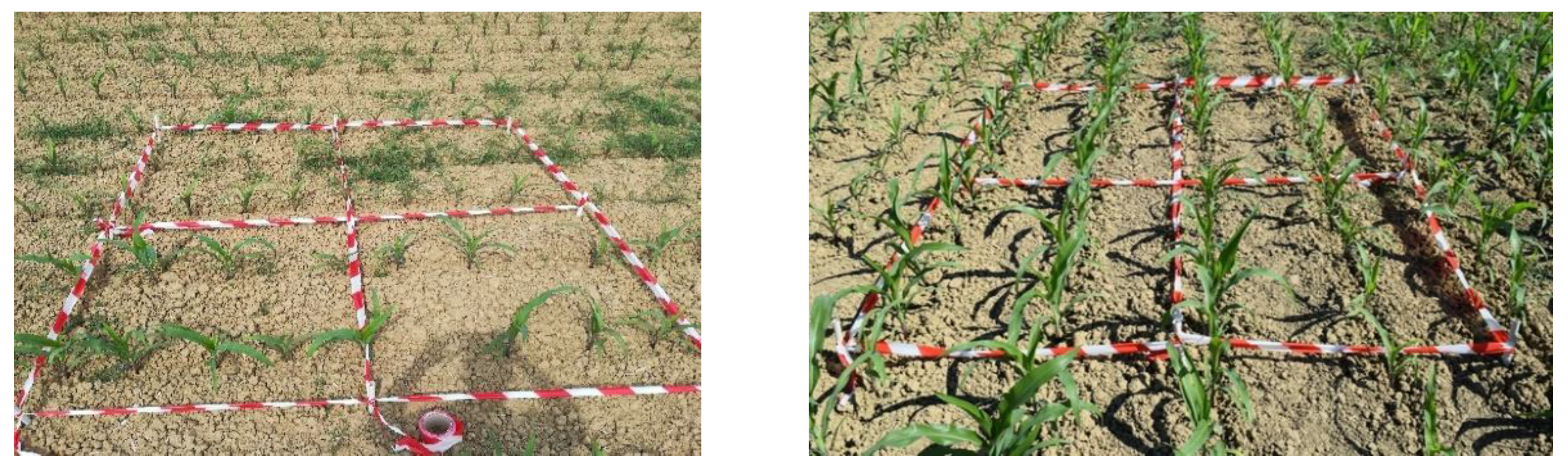
Eight plots of 4 m² (2.0 m × 2.0 m) were set up, each containing four rows of maize plants (Figure 1).

At the 4–5 leaf stage, the number of plants of maize (NM) and weeds (NW) was counted on each plot. Afterwards, half of the plots were weeded (weeded plots = WP) by using 0.5 l ha⁻¹ of Aric 480 L.S. (41% Dicamba) and 1.5 l ha⁻¹ of Nifuron (4.18% Nicosolfuron), whereas no intervention was carried out on the remaining four plots (control plots = CP). At harvest time, the aboveground biomass of all maize plants was collected from each plot (WP and CP) and weighed after oven drying at 60 °C until constant weight. On the other four plots of 4 m² (2.0 m × 2.0 m), the number of maize plants was counted and all weeds were removed manually before the UAV flight (pulling weed plots = PWP) in order to estimate more easily the average cover value of a single maize plant.

The UAV flight was made on the 25th of June over the entire surface of both fields, just before the weed and crop scouting. We used the drone “Agri-Efesto”, made available by Sigma Ingegneria and the Precision Agriculture group of the CNR-IBIMET of Florence. The drone was a modified multi-rotor Mikrokopter (HiSystems GmbH, Moomerland, Germany) with six MK3538 and APC propellers 12 × 3.8 inches. Autonomous fight through a predefined route was set using the onboard navigation system based on a GPS receiver (U-blox LEA6S) connected to a navigation board (Navy-Ctrl 2.0) and a small Microelectromechanical System (MEMS)-based IMU (Inertial Measurement Unit) (Mikrokopter Flight Controller ME V2.1). A universal camera mount equipped with three servomotors permitted accurate image acquisition through the compensation for tilt and rolling effects. The Agri-Efesto was equipped with a Sony Cyber-shot DSC-QX100 RGB camera (Sony Corporation, Tokyo, Japan), which mounts a 20.2-megapixel CMOS Exmor R sensor and a Carl Zeiss Vario-Sonnar T lens.

The UAV flight was made at 10 and 20 m in height, with a ground-size pixel equal to 3.5 mm and 7.1 mm, respectively, maintaining an overlap of 70% between the individual frames.

2.3. Image Processing

The RGB images of experimental plots acquired from the UAV were orthorectified and mosaicked using Agisoft Photoscan Professional Edition 1.1.6 (Agisoft LLC, St. Petersburg, Russia).

The orthomosaic was processed with Canopeo, which analyses images by using colour values in the red (R), green (G) and blue (B) system and classifies all pixels according to three selection parameters: R/G, B/G and the green excess index (GEI = 2G-R-B) [36,37,38,39]. The starting image was turned into a binary image depending on whether the pixels met the selection criteria or not (R/G < 0.95, B/G < 0.95, and GEI > 20, default values). In this way, we obtained the total green cover for the WP and CP (Ca-TGC_WP+CP).

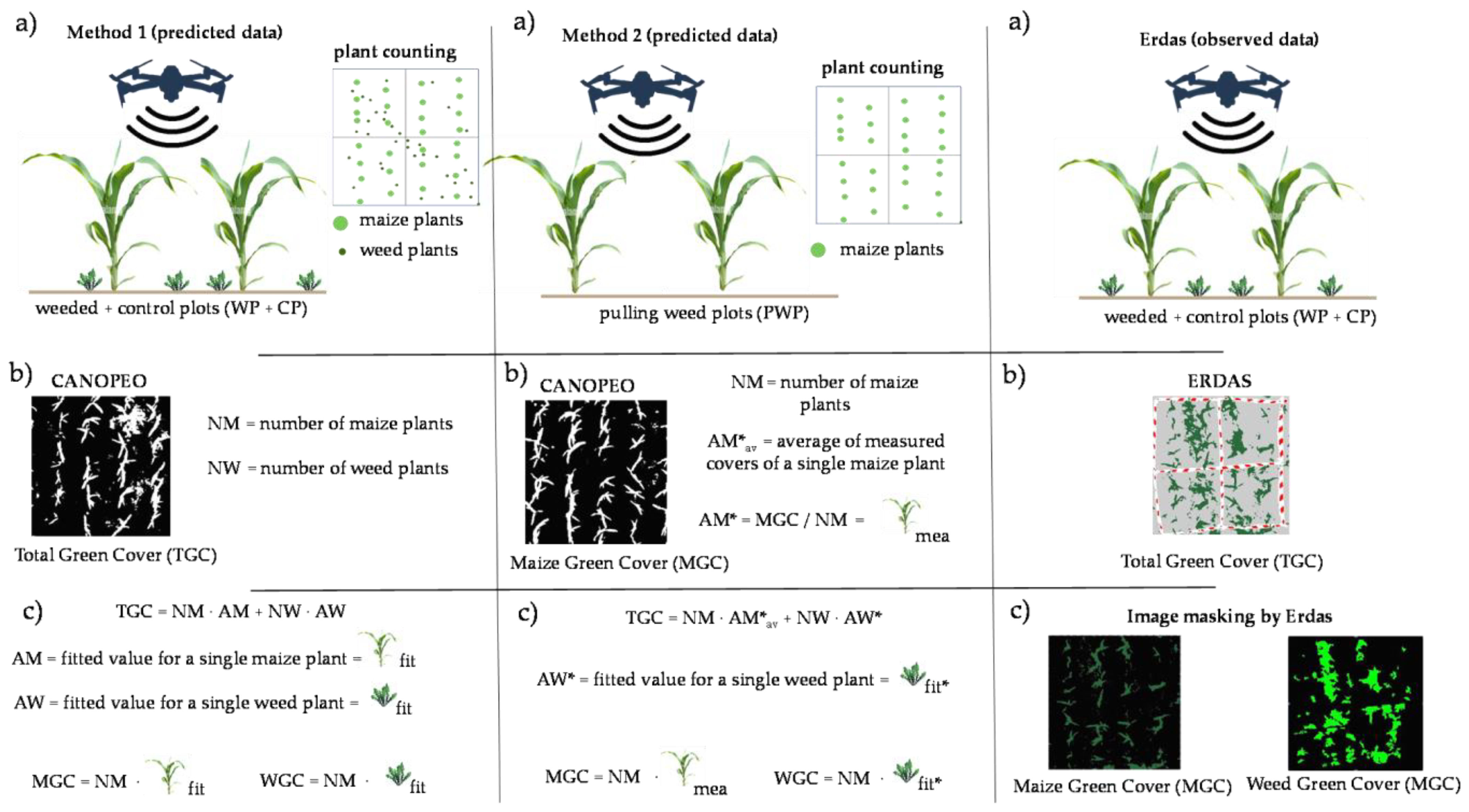
In order to estimate the values of MGC and WGC for the WP and CP, we tested two different methods. In the first method (M1), we expressed the Ca-TGC_WP+CP as the sum of MGC_WP+CP and WGC_WP+CP (1) and they, in turn, are expressed as the product of the number of maize/weed plants by the average cover of a single plant of maize/weed (2) and (3) (Figure 2).

Ca − TGC_WP+CP = MGC_WP+CP + WCG_WP+CP

(1)

MGC_WP+CP = NM_WP+CP × AM_WP+CP

(2)

WGC_WP+CP = NW_WP+CP × AW_WP+CP

(3)

Ca − TGC_WP+CP = NM_WP+CP × AM_WP+CP + NW_WP+CP × AW_WP+CP

(4)

where Ca-TGC_WP+CP were the values obtained by processing the UAV images with Canopeo, NM_WP+CP = the number of maize plants counted in the WP and CP, AM_WP+CP = the average cover of a single maize plant, NW_WP+CP = the number of weed plants counted in the WP and CP, and AW_WP+CP = the average cover of a single weed plant.

At this point, we used a linear least-squares fitting (n = 8) to find the best values for the AM_WP+CP (AM) and for the AW_WP+CP (AW) able to approximate Equation (4), and to solve Equations (5) and (6):

M1 − MGC_WP+CP = NM_WP+CP × AM

(5)

M1 − WGC_WP+CP = NW_WP+CP × AW

(6)

In the second method (M2), we estimated the value of AM (AM*) by using the images captured of the PWP. We assumed that the development of the maize plants was very similar within the experimental fields (sown all on the same day), therefore, we can estimate the value of AM by dividing the Ca-TGC data measured with Canopeo on the PWP (Ca-TGC_PWP) by the corresponding number of maize plants NM_PWP (7). Indeed, the Ca-TGC_PWP corresponded to the Ca-MGC_PWP values since, in the PWP, all weeds had been removed manually. Afterwards, we calculated the average of the AM* values obtained for each PWP ($\overline{\mathrm{AM}}$*) (8).

AM* = Ca − TGC_PWP/NM_PWP

(7)

$$\overline{\mathrm{AM}}*=\mathrm{average} \mathrm{of} \mathrm{AM}* (1,\dots 4)$$

(8)

We replaced the AM with the $\overline{\mathrm{AM}}$* in (4) to obtain a new equation to express the TGC_WP+CP (9).

$${\mathrm{Ca-TGC}}_{\mathrm{WP}+\mathrm{CP} }={\mathrm{NM}}_{\mathrm{WP}+\mathrm{CP}}\times \overline{\mathrm{AM}}*+{\mathrm{NW}}_{\mathrm{WP}+\mathrm{CP} }\times {\mathrm{AW}*}_{\mathrm{WP}+\mathrm{CP}}$$

(9)

We approximated the value of AW* in Equation (9) by means of linear least-squares fitting (n = 8) and, therefore, we estimated the value of weed green cover according to the M2 (M2-WGC_WP+CP) by using Equation (10).

M2 − WGC_WP+CP = NW_WP+CP × AW*

(10)

For both methods, the estimates of AM and AW and AW* were performed using Microsoft Excel Solver according to the trial-and-error approach [40].

2.4. Determination of the Economic Threshold (ET)

The relationship between the WGC and the Relative Yield Loss (RYL) of maize was computed according to [21] who adapted the two-parameter regression model proposed by [41] to obtain the Equations (11) and (12), which relate RYL (expressed as a ratio to the maximum yield) and WGC (expressed as a ratio to the total area):

$$\mathrm{RYL}=\frac{q\times \mathrm{WGC}}{1+\left(q/m-1\right) \mathrm{WGC}}$$

(11)

$$\mathrm{WGC}=\frac{\mathrm{RYL}}{q-\left(q/m-1\right) \mathrm{RYL}}$$

(12)

where q is the damage coefficient attributed to the weed population and m represents the maximum yield loss that occurred when the weed cover reaches the highest possible value (WGC = 1).

The values of q and m chosen for the calculation of Equation (11) were q = 2.5 and m = 0.70 (RYL = 2.5 WGC/1 + 2.57 WGC, curve 1 = C1). The values of q and m are consistent with the literature [21] and were calibrated by considering the site-specific conditions of the experimentation. The estimated values of RYL were calculated by substituting, in C1, the values of WGC obtained with the two methods (M1-WGC_WP+CP and M2-WGC_WP+CP).

We calculated the other two curves from Equation (11): curve 2 (C2) with q = 3.7 and m = 0.39, obtained by fitting the two parameters by using the data from the M2-WGC_CP at 10 m, and curve 3 (C3) with q = 6.2 and m = 0.32 obtained by fitting the two parameters using the data from Er-WGC_CP at 10 m. These two curves were used only to make a comparison with the economic threshold values obtained by using C1.

The costs of weeding were estimated by summing the current price of herbicides used (49.00 € ha⁻¹) and the rate of local contractors for spraying (66.00 € ha⁻¹). Earnings were based on the local price of silage maize (at 33% of moisture) recorded at the time of the experimental period.

2.5. Reliability of the Proposed Methods

To evaluate the consistency of the proposed method in estimating the different green cover types (TGC, CGC and WGC), we processed the same images captured by UAV using Erdas Imagine software by Hexagon AB, which can classify images by supporting both supervised or unsupervised procedures [42].

Firstly, we used Erdas to turn the original images into binary images (green and non-green cover) by using an unsupervised procedure based on parameter settings similar to that used for Canopeo. The obtained values (Er-TGC_WP+CP) were compared to those from Canopeo by using the t-test for paired samples and the Pearson correlation coefficient (r).

To discriminate between the two types of green cover, we could not use an unsupervised procedure based on a signature set since the spectral patterns of maize and weed are very similar to each other. Therefore, we started again from the original images (Figure 3a) where we masked the pixels belonging to maize manually by zooming in and out until the attribution was certain (Figure 3b). Afterwards, we classified the rest of the image by applying the signature set used for the TGC determination so as to obtain the weed green cover (Er-WGC_WP+CP) (Figure 3c). The reverse procedure was followed for the maize green cover calculation (Er-MGC_WP+CP).

The comparison between the estimates obtained by using the two proposed methods (M1 and M2) and the results of the image processing by Erdas was reliable, even in this case, with the t-test for paired samples and the Pearson correlation coefficient (r).

The goodness of fit used to calibrate the parameters of the two estimation methods (AM and AW for M1 and AW* for M2) was evaluated by comparing the obtained values of the MGC and WGC (predicted data) with the Er-MGC_WP+CP and Er-WGC_WP+CP (observed data) (n = 8). In the case of RYL, we used the values obtained from Equation (12) as the predicted data, and the values of RYL were calculated by subtracting the yield of each CP as observed data (n = 4) from the maximum maize yields (assumed equal to the average of yields of the WP).

The model quality indices used are reported in

Table 1. The indices used to evaluate the goodness of fit (P_i = estimated values, O_i = observed values, Ō = the average of observed data, and n = number of the observations).

Quality Indices	Formula	Optimum
Root Mean Square Error	$RMSE={[{\displaystyle \sum }_{i=1}^n\left(P_i-O_{i }\right)/n]}^{0,5}$	0
	$RMSE/Ō={[{\displaystyle \sum }_{i=1}^n\left(P_i-O_{i }\right)/n]}^{0,5}*100/Ō$	0
Mean Absolute Error	$MAE={\displaystyle \sum }_{i=1}^n\left|P_i-O_i\right|$	0
Modelling Efficiency	$EF=({\displaystyle \sum }_{i=1}^n{(O_i-Ō)}^2-{\displaystyle \sum }_{i=1}^n{(P_i-O_i)}^2/{\displaystyle \sum }_{i=1}^n\left(O_i-Ō\right)$	1
Coefficient Residual Mass	$CRM=\left({\displaystyle \sum }_{i=1}^n{O}_i-{\displaystyle \sum }_{i=1}^n{P}_i\right)/{\displaystyle \sum }_{i=1}^n{O}_i$	0

, e.g., RMSE (Root Mean Square Error), RMSE/Ō (where Ō is the average of the observed data), MAE (Mean Absolute Error), EF (Modelling Efficiency), and CRM (Coefficient of Residual Mass) [43].

3. Results

The results of the TGC measured with Canopeo were very close to those obtained with Erdas (

Table 2. Total green cover in weeded and control plots (WP and CP) was obtained using Canopeo (Ca-TGC_WP+CP) and Erdas (Er-TGC_WP+CP). Student t-test, p-value and Pearson correlation coefficient (r).

Flight Height (m)	Ca-TGCWP+CP (m2)	Er-TGCWP+CP (m2)	Stat t	p	r
10	0.95	0.92	0.520	0.619	0.87 **
20	1.05	1.19	−1.844	0.108	0.90 **

(** = p < 0.01).

). The results from the two software methods were not statistically different, neither at 10 m (p = 0.619), nor 20 m (p = 0.108), and the deviation measured ranged, in absolute value terms, from 3 to 12%. The Pearson correlation coefficient was very high in both cases (r = 0.87 and 0.90 for 10 and 20 m, respectively, p < 0.01).

In

Table 3. Maize green cover and weed green cover on weeded and control plots (WP and CP) obtained using method 1 (M1-MGC_WP+CP and M1-WGC_WP+CP) and Erdas (Er-MGC_WP+CP and Er-WGC_WP+CP). Student t-test, p-value and Pearson correlation coefficient (r).

Flight Height (m)	M1-MGCWP+CP (m2)	Er-MGCWP+CP (m2)	Stat t	p	r
10	0.60	0.75	−5.660	0.001	0.36 ns
20	0.73	1.05	−3.486	0.010	0.06 ns
Flight Height (m)	M1-WGCWP+CP (m2)	Er-WGCWP+CP (m2)	Stat t	p	r
10	0.35	0.17	4.777	0.002	0.94 **
20	0.33	0.14	5.296	0.001	0.91 **

(ns = not significant, ** = p < 0.01).

, the values of the M1-MGC_WP+CP and M1-WCG_WP+CP are compared with those obtained from Erdas for the same plots. The estimated values were significantly different from Er-MGC_WP+CP and Er-WGC_WP+CP at both 10 and 20 m. In particular, M1-MGC_WP+CP underestimated the values of Erdas by 0.15 m² (−20%) and 0.32 m² (−30%), at 10 and 20 m, respectively. Moreover, the correlation levels between estimated and measured values were very low at 10 m (r = 0.36) or nonexistent at 20 m (r = 0.06). Conversely, we observed a better correlation between the M1-WGC_WP+CP and the Er-WGC_WP+CP, even if the two quantities remain statistically different from each other for both the flight heights, the deviation was still larger (+106 and +136%, for 10 and 20 m, respectively), than that observed for the maize. Instead, the resulting values of r were very high (significant for p < 0.01), equal to 0.94 and 0.91 for 10 and 20 m, respectively.

Moving on to M2 (

Table 4. Maize green cover and weed green cover in weeded and control plots (WP and CP) obtained using method 1 (M2-MGC_WP+CP and M2-WGC_WP+CP) and Erdas (Er-MGC_WP+CP and Er-WGC_WP+CP) (Student t-test).

Flight Height (m)	M2-MGCWP+CP (m2)	Er-MGCWP+CP (m2)	Stat t	p	r
10	0.76	0.75	0.386	0.711	0.36 ns
20	0.94	1.05	−1.172	0.280	0.06 ns
Flight Height (m)	M2-WGCWP+CP (m2)	Er-WGCWP+CP (m2)	Stat t	p	r
10	0.24	0.17	3.311	0.013	0.94 **
20	0.17	0.14	1.689	0.135	0.91 **

(ns = not significant, ** = p < 0.01).

), the values of the M2-MGC_WP+CP results were statically equivalent to those from Erdas at both 10 (p = 0.71) and 20 m (p = 0.28), whereas the Pearson correlation coefficient results were not significant. The values of r were the same calculated for M1-MGC_WP+CP since they were obtained as the product of NM_WP+CP by a constant value (AM for M1 and AM* for M2). In addition, the resulting differences between M2-WGC_WP+CP and Er-WGC_WP+CP were further reduced. At 10 m, the deviation was equal to +0.01 m² (+1%) and −0.11 m² (−10%) for 10 and 20 m, respectively. These values implied statistical significance for the former (p = 0.013), but not for the latter (p = 0.135). The values of r were, in both cases, high (r > 0.90) and significant at (p < 0.01) (the values of r, were, even in this case, equal to those calculated for M2-WGC_WP+CP for the same reason reported above).

The indices used to evaluate the goodness of fit confirmed the previous results. The values of M1 (

Table 5. Modelling quality indices (RMSE, RMSE/Ō, MAE, EF and CRM for more details see Table 1) used to evaluate the goodness of fit for method 1 (M1) at 10 and 20 m of flight height in estimating the maize green cover (MGC), the weed green cover (WGC) and relative yield loss (RYL).

Quality Indices	M1 at 10 m of Flight Height			M1 at 20 m of Flight Height
	MGC	WGC	RYL	MGC	WGC	RYL
RMSE	0.20	0.17	0.07	0.21	0.40	0.06
RMSE/O	119	22	40	158	38	35
MAE	1.43	1.22	0.20	1.53	2.95	0.19
EF	−1.07	−3.85	−0.40	−1.28	−1.74	−0.05
CRM	−1.04	0.20	−0.27	−1.41	0.31	−0.20

) calculated at 10 m were disappointing both for the MGC (MAE = 1.22 m², EF = −3.85) and for the WCG (RMSE/ Ō = 119%, MAE = 1.43 m², CRM = −1.04, EF = −1.07). At 20 m, almost all indices of M1 worsened, especially those related to the WCG (RMSE/ Ō = 158%, MAE = 1.53 m², CRM = −1.41, EF = −1.28). The indices calculated for RYL at 10 m were not much better (RMSE/Ō = 40%, EF = −0.40, CRM = −0.27) but, in this case, the fitting improved when passing at 20 m (RMSE/Ō = 35%, EF = −0.05, CRM = −0.20).

Good values of indices were reached only by using M2 (

Table 6. Modelling quality indices (RMSE, RMSE/Ō, MAE, EF and CRM for more details see Table 1) used to evaluate the goodness of fit for method 2 (M2) at 10 and 20 m of flight height in estimating the maize green cover (MGC), the weed green cover (WGC) and relative yield loss (RYL).

Quality Indices	M2 at 10 m of Flight Height			M2 at 20 m of Flight Height
	MGC	WGC	RYL	MGC	WGC	RYL
RMSE	0.08	0.07	0.04	0.07	0.27	0.05
RMSE/O	48	10	25	55	26	40
MAE	0.61	0.42	0.15	0.53	1.76	0.15
EF	0.66	0.10	0.48	0.73	−0.21	0.16
CRM	−0.38	−0.01	0.07	−0.29	0.10	0.31

), especially for the WCG. At 10 m, the results obtained were already acceptable (RMSE = 0.08, MAE = 0.61 m², EF = 0.66) and they became even better at 20 m (RMSE = 0.07, MAE = 0.53 m², EF = 0.73). Conversely, the trend drawn by RYL was the opposite as, at 10 m, the values of the indices were better than at 20 m (RMSE/Ō = 25 and 40%, EF = 0.48 and 0.16, CRM = 0.07 and 0.31 for 10 and 20 m, respectively).

The curve obtained from Equation (11) using the calibrated values of q and m (2.5 and 0.70, respectively), in order to model the relationship between WGC and RYL, is reported in Figure 4, together with the points defined by the values of M1-WGC_CP or M2-WGC_CP (as abscissa) and by the values of RYL measured in each CP (as ordinate), at both 10 and 20 m. The vertical distance of these points from the curve is a measure of the inaccuracy of the model in estimating the RYL, starting from the values of WGC obtained using M1 and M2. The point distribution pattern confirmed the trend observed previously, namely that fitting with the RYL observed data improved for M1 passing from 10 to 20 m, whereas for M2, we observed an opposite behaviour.

In Figure 5, the determination of the economic threshold (ET) is reported for the three different types of curves obtained from Equation (10). The values found by using C1, C2 and C3 were, respectively, equal to 0.0024 (ET-C1), 0.0020 (ET-C2) and 0.0016 (ET-C3) of the investigated area.

4. Discussion

The first critical point in the study of weed and crop cover is linked to the determination and the availability of “true values”. It is not easy to obtain an accurate measurement of the plant cover because of difficulties in performing a direct measurement (e.g., by using tools such as planimeters) and in turning the surface values into cover values.

In the end, image processing remains the more feasible method to measure plant cover, and the possibility of manually segmenting images, which the software provides, allows users to reach an adequate level of accuracy. Moreover, it is reasonable to assume that any inaccuracies in image segmentation are regularly distributed and therefore they are not able to substantially alter the results. In our study, the equivalency of the TCG values obtained with Canopeo and Erdas provided an additional element of confirmation in the consistency of these methods [44,45].

A different matter, on the other hand, concerns the discrimination between crops and weeds, since the use of spectral information, especially if only RGB images are available, does not provide sufficient information to distinguish one plant species from another. In the early stages of growth, it is particularly difficult to discriminate between crops and weeds, since both have similar reflectance characteristics [46,47]. This can be a serious barrier for farmers who intend to adopt the economic threshold, as a rule, to manage post-emergence weeding, since, as reported by various authors [22,48,49,50], the estimation of the weed cover seems to be the best proxy to evaluate the infestation level in a field and to consequently act.

The first of the two proposed methods (M1), based on the joint estimation of the two parameters (AM and AW) showed poor accuracy and reliability in estimating the maize green cover (underestimated) and the weed green cover (overestimated), as also reported by other authors who followed a similar approach [27,51]. These failures are probably due to the high variability in the green cover of each single weed plant if compared to that of maize plants. Only the use of a great number of images (and of the respective counts of maize and weed plants) could allow us to better calibrate AM and AW and reduce the inaccuracy.

The second method proposed seems to be more promising. The estimate of the AM based on a different dataset, allowed by the high homogeneity in maize plant growth, and the consequent subtraction of the M2-MGC_WP+CP from the Ca-TGC_WP+CP reduced the uncertainty in the estimate of the M2-WGC_WP+CP, improving the fitting efficacy with respect to both Er-WGC_WP+CP (EF = 0.66 at 10 m) and RYL (EF = 0.48 at 10 m). The large variability in cover values for weed plants was again the main reason for the discrepancy between predicted and observed values. Image acquisition in an earlier stage of the crop development could reduce the heterogeneity of weed cover values (since newly emerged weeds should have less variability), but there would be the risk of neglecting all the weeds that could emerge later.

Regarding the relationship between WGC and RYL, this changes in relation to the weed species composition, the crop type and vigour, and the soil and climatic conditions [22,50,52]. The q and m values of Equation (10) have to be properly calibrated for site-specific conditions. For instance, it would be useful to define the parameters q and m for the main common types of weed community [21], even if this requires experimental activities on site.

Regarding the influence of flight height, the reduction in the ground resolution of the processed images passing from 10 to 20 m led to a further loss in accuracy for the M1 and a slight improvement for the M2-WGC_WP+CP and a limited worsening for the M2-MGC_WP+CP. This means that the degradation of images made in the joint estimation of AM and AW are even less accurate, whereas the increase in the Ca-TGC_PWP and consequently in the M2-MGC_WP+CP estimation at 20 m had the effect of bringing M2-WGC_WP+CP (underestimated at 10 m) closer to the observed data. The improvement in the M2-WGC_WP+CP estimation at 20 m did not lead to an improvement of RYL fitting, probably because of too high a value attributed to q (the damage coefficient of the weed population).

Finally, the determination of the economic threshold using the three curves (C1, C2 and C3) did not lead to great differences. The deviation between ET-C2 and ET-C1 was equal to −16% and the deviation between ET-C3 and ET-C1 was equal to −33%, but the values attributed to the q and m parameters in C2 and C3 seem to hardly be justified.

From a technical point of view, the solution of using M2 at 20 m may be acceptable in usual farming practices in relation to a remarkable reduction (about one-half) of the flight times.

5. Conclusions

The use of simple and inexpensive methods may be a valuable aid in the penetration of precision farming techniques, even for smaller farms. The greatest difficulties that farmers meet in using these types of technologies are mainly concerned with the lack of tools that are able to interpret the data acquired through remote sensing to provide clear information for the management of farming practices.

The proposed method allows farmers to more rationally manage post-emergence weeding by providing the theoretical basis to compute the economic threshold by using simple calculation elements available on any spreadsheet software and a free downloadable app.

The critical points concern the great variability in shape and size of weed species that make it difficult to estimate their cover, starting with their number. In addition, the manual counting of weed plants can pose some problems due to the experience and subjectivity of the user (for instance, the minimum size above which the plant must be counted). Moreover, the weed emergence will scale over time and consequently, the definition of the competition coefficient (q) can change significantly. In this regard, it should be emphasized that the calibration of the RYL models on the site where they are to be applied represents a fundamental requirement for their correct use.