Omni-Directional Semi-Global Stereo Matching with Reliable Information Propagation

Abstract

High efficiency and accuracy of semi-global matching (SGM) make it widely used in many stereo vision applications. However, SGM not only struggles in dealing with pixels in homogeneous area, but also suffers from streak artifacts. In this paper, we propose a novel omni-directional SGM (OmniSGM) with a cost volume update scheme to aggregate costs from paths along all directions and to encourage reliable information to propagate across entire image. Specifically, we perform SGM along four tree structures, namely trees in the left, right, top and bottom of root node, and then fuse the outputs to obtain final result. The contributions of pixels on each tree can be recursively computed from leaf nodes to root node, ensuring our method has linear time computational complexity. Moreover, An iterative cost volume update scheme is proposed using aggregated cost in the last pass to enhance the robustness of initial matching cost. Thus, useful information is more likely to propagate in a long distance to handle the ambiguities in low textural area. Finally, we present an efficient strategy to propagate disparities of stable pixels along the minimum spanning tree (MST) for disparity refinement. Extensive experiments in stereo matching on Middlebury and KITTI datasets demonstrate that our method outperforms typical traditional SGM-based cost aggregation methods.

1. Introduction

Stereo correspondence serves as a fundamental building block in many computer vision tasks, such as 3D reconstruction, navigation, and recognition [1,2,3], and has been extensively studied in last two decades. Typical procedures to decide matching pixels in two rectified stereo pairs are building cost volume for reference image at all candidate disparities, aggregating cost in a neighborhood to filter out noise, assigning a label to each pixel and post-process to enhance the result. The aim of these procedures is to find a locally smooth solution in which discontinuities are aligned with the edges in reference image. Traditional stereo matching approaches can be categorized into local filtering [4,5,6,7,8] and global optimization approaches [9,10,11,12].

Local filtering methods estimate the weighted average or sum of matching costs in a support window, and the weights between neighboring pixels depend on the intensity similarity and the spatial affinity. Local edge-aware filters, for instance the bilateral filter (BF) [13] and the guided filter (GF) [14], produce appealing results for highly textured images. However, these methods incorporate information in a local support region which is not geometric adaptive and cannot properly handle pixels in homogeneous regions. In order to aggregate information in the whole image, Yang [7,15] proposed the non-local filter (NL) which treats reference image as an undirected, 4-connected graph and extracts a minimum spanning tree from this graph by removing edges with large gradients. The aggregation procedure can be implemented by traversing the MST in two passes, namely from leaf nodes to root node and then from root node to leaf nodes. Segment-tree (ST) built by Mei et al. [16] aims to enforce tight connections for pixels in a local region, while the structure of tree used for propagating message heavily depends on super-pixel segmentation [17]. The recursive non-local filter (RNLF) [18] builds four trees for input image based on the relative spatial relationships of neighboring pixels. The Chebyshev distance is used to compute the weight between any two pixels. However, the intensity distance between any two pixels on the tree is much larger than the intensity difference of these two pixels. Therefore, weights in highly textured regions decrease rapidly as the spatial distance increases, inhibiting informative messages from being propagated in wide range. Although those cost filtering methods produce appealing results for highly textured stereo pairs, they suffer from resolving the ambiguity in homogeneous regions or tend to overuse piece-wise constant assumption.

Global methods attempt to minimize a global energy function which composed by two terms, data term and smoothness term. Data term ensures the proximity of two matching pixels while the smoothness term enforces the discontinuities in disparity image aligned with edges in the reference image. A popular approach to solve this energy function is utilizing graph-based energy minimization methods in Markov Random Field (MRF) framework [19,20], for example graph cut (GC) [10,11] and belief propagation (BP) [12,21]. These methods treat reference image as an undirected graph and pass messages across entire graph to maximize a posterior estimation (MAP). Although many improvements have been made to enhance the efficiency or to accelerate the convergence rate of those global methods, they are still computationally intensive.

Semi-global stereo matching [22] is an efficient strategy to solve an global energy function by approximating a 2D MRF minimization with multiple 1D optimizations. Inference along each scan line is performed separately, and the outputs in multiple directions are fused to determine the label of each pixel. As the 1D optimization operations along multiple scan lines in each pass are independent with each other, several approaches [23,24,25,26,27,28] take advantage of field-programmable gate-array (FPGA) or graphics card (GPU) to accelerate SGM in real-time applications. However, only pixels on scan lines intersected at current pixel in the reference image contribute to the aggregated cost of root node, degrading the performance of SGM under challenging conditions. Another shortcoming of SGM is that two adjacent pixels only share pixels on the same scan line. When matching costs on this line is unreliable, messages from other directions would produce different results for these pixels, resulting in stripe artifacts in disparity image. SGM-forest [29] treats solutions in multiple directions as independent disparity proposals and formulate the fusion procedure as a classification problem that chooses the optimal estimate from given proposals. MGM [30] takes messages from the nodes visited in previous scan line into account, aiming to make full use of information in 2D dimensions in cost aggregation along the 1D path. It overemphasizes information in neighboring pixels and inhibits an informative message from being propagated in a wide range to handle pixels in weakly textured area. Tripe SGM [31] extends SGM to three images from a triplet-stereo rig which are composed by a horizontal and vertical camera pair. SGM-Net [32] learns the penalties between neighboring pixels using Convolutional Neural Networks (CNN). In our approach, useful information is propagated in a certian direction along each tree and all pixels on the tree contribute to the aggregated cost of root node, making our method not only reduce streak artifacts of traditional SGM but also alleviate the ambiguities in homogeneous region.

In this paper, we propose a new version of SGM, named omni-directional SGM (OmniSGM), which acts as performing 1D optimization along all directions. We also present an iterative cost update scheme utilizing aggregated cost in the last pass to successfully improve the robustness of initial matching cost. Specifically, our method performs SGM along tree structures in four directions, namely from left-to-right, right-to-left, top-to-bottom and bottom-to-top, as shown in the last row of Figure 1. In each pass, we recursively estimate the contribution of each pixel on the tree from leaf nodes to root node, leading to all pixels on the tree contribute to the aggregated cost of root node. Then we fuse the outputs of these four trees to obtain the final aggregated cost; thus, each pixel obtains supports from pixels in the whole image, making our method alleviate some limitations of SGM, such as streak artifacts. Compared with SGM-based methods which incorporate information from multiple scan lines, our method can be regarded as aggregating information from all pixels along all directions. In order to fully exploit reliable information in aggregated cost volume, we integrate it with initial cost volume according to the confidence of each pixel. With this successive cost volume update scheme, initial cost volume becomes more robust, and reliable information tends to propagate extensively across entire image. In the post-process step, we advance the widely used non-local refinement method [15] to efficiently propagate disparities from stable pixels to unstable pixels.

The rest of this paper is organized as follows. In Section 2, we present an introduction of traditional semi-global matching method at first, and then elaborate our proposed omni-directional SGM, cost volume update scheme and the efficient refinement strategy. Parameter settings and extensive experiments on widely used data sets are provided in Section 3. Conclusions and remarks are given in Section 4.

2. Omni-Directional SGM with Reliable Cost Propagation

In this section, we first give a explanation of traditional SGM algorithm and then elaborate our proposed omni-directional SGM, cost volume update scheme and the efficient stable disparity propagation strategy.

2.1. Semi-Global Matching

SGM utilizes multiple efficient 1D optimizations to approximately minimize the 2D global energy function utilizing 2D Markov Random Field. The global energy function $E\left(D\right)$ is defined by

$$E\left(D\right)=\sum _{\mathit{p}}(C(\mathit{p},d^{\mathit{p}})+\sum _{\mathit{q}\in N\left(\mathit{p}\right)}{P}_{1}T\left[\right|d^{\mathit{p}}-d^{\mathit{q}}|=1]+\sum _{\mathit{q}\in N\left(\mathit{p}\right)}{P}_{2}T\left[\right|d^{\mathit{p}}-d^{\mathit{q}}|>1])$$

(1)

where $C(\mathit{p},d^{\mathit{p}})$ represents the matching cost of pixel $\mathit{p}$ at disparity $d^{\mathit{p}}$. The first term is the sum of matching costs for all pixels in reference image at disparities D. The second term is the constant penalty $P_1$ for pixels in slant surface in the neighborhood $N\left(\mathit{p}\right)$ of $\mathit{p}$. The third term adds a larger penalty $P_2$ for discontinuities in disparity image. Discontinuities often align with intensity changes, since $P_2$ depends on the magnitude of image gradient, such as $P_2=P_2^{{}^{\prime }}/|I\left(\mathit{p}\right)-I\left(\mathit{q}\right)|$. $T[.]$ represents Kronecker delta function which is 1 when the condition in the bracket is satisfied, otherwise 0.

In order to minimize $E\left(D\right)$, SGM computes the aggregated cost of pixel $\mathit{p}$ at disparity d by summing the costs of multiple 1D minimum cost paths ended at pixel $\mathit{p}$ at disparity d. The aggregated cost $L_{\mathit{r}}^{{}^{\prime }}(\mathit{p},d)$ along the path in direction $\mathit{r}$ for pixel $\mathit{p}$ at disparity d can be recursively computed by

$$\begin{array}{cc}\hfill L_{\mathit{r}}^{{}^{\prime }}(\mathit{p},d)=& C(\mathit{p},d)+\min (L_{\mathit{r}}^{{}^{\prime }}(\mathit{p}-\mathit{r},d),L_{\mathit{r}}^{{}^{\prime }}(\mathit{p}-\mathit{r},d-1)+P_1,L_{\mathit{r}}^{{}^{\prime }}(\mathit{p}-\mathit{r},d+1)+P_1,\hfill \\ \hfill & \underset{l}{\min }{L}_{\mathit{r}}^{{}^{\prime }}(\mathit{p}-\mathit{r},l)+P_2)\hfill \end{array}$$

(2)

For simplicity, we use $V(d,d^{{}^{\prime }})$ to denote the pair-wise first-order smoothness assumption that penalizes disparity differences between neighboring pixels in Equations (1) and (2), which is

$$V(d,d^{{}^{\prime }})=\left\{\begin{array}{cc}0\hfill & \mathrm{if}d=d^{{}^{\prime }}\hfill \\ P_1\hfill & \mathrm{if}|d-d^{{}^{\prime }}|=1\hfill \\ P_2\hfill & \mathrm{if}|d-d^{{}^{\prime }}|>1\hfill \end{array}\right.$$

Since $L_{\mathit{r}}^{{}^{\prime }}(\mathit{p},d)$ can be reformulated by

$$L_{\mathit{r}}^{{}^{\prime }}(\mathit{p},d)=C(\mathit{p},d)+\underset{d}{\min }(L_{\mathit{r}}^{{}^{\prime }}(\mathit{p}-\mathit{r},d)+V(d,d^{{}^{\prime }}))$$

(3)

As $L_{\mathit{r}}^{{}^{\prime }}(\mathit{p},d)$ could increase to a very large value due to successive accumulation along the path, thus the minimum cost of previous pixel is subtracted. As the subtracted value is a constant for all disparities at each pixel, since it does not change the actual path in disparity space. The modified aggregated cost along direction r can be expressed as

$$L_{\mathit{r}}(\mathit{p},d)=C(\mathit{p},d)+\underset{d}{\min }(L_{\mathit{r}}(\mathit{p}-\mathit{r},d)+V(d,d^{{}^{\prime }}))-\underset{k}{\min }{L}_{\mathit{r}}(\mathit{p}-\mathit{r},k)$$

(4)

The final aggregated cost is the sum of $L_{\mathit{r}}$ at all directions, and the disparity image is decided by the winner-take-all (WTA) strategy as

$$D\left(\mathit{p}\right)=\arg \underset{d}{\min }\sum _{\mathit{r}}{L}_{\mathit{r}}(\mathit{p},d)$$

(5)

2.2. Omni-Directional SGM

Traditional SGM only takes pixels on several scan lines into account, and MGM tries to remove streak artifacts in disparity image by incorporating messages from nodes visited in the previous scan line. However, pixels in the neighborhood of root node contribute to the aggregated cost of root node multiple times in MGM (there are multiple paths between these two nodes), making pixels in the neighborhood overweight compared to other pixels and inhibiting reliable information from being propagated across the reference image, as shown in the second row of Figure 1. Here we propose omni-directional SGM which owns several advantages: (1) all pixels in the reference image contribute to the aggregated cost of root node; (2) there is only one path between any two pixels; (3) information propagates along all directions to alleviate streak artifacts; (4) aggregated cost can be recursively computed in linear time in each pass. As shown in the last row of Figure 1, our method traverses the reference image along four directions, namely from left-to-right, right-to-left, top-to-bottom and bottom-to-top. In each pass, the aggregated cost of root node can be recursively calculated from leaf nodes to root node.

2.2.1. Cost Aggregation on Each Tree

Here we use ${\mathit{r}}^k\in \{(1,0),(-1,0),(0,1),(0,-1)\},k=1,2,3,4$ to denote the directions of four tree structures, and use ${\mathit{r}}^{k+}$ and ${\mathit{r}}^{k-}$ to denote the positions of child nodes in diagonal directions, as shown in Figure 2. For instance, if we perform cost aggregation from left-to-right, so we have ${\mathit{r}}^k=(1,0)$, ${\mathit{r}}^{k+}=(1,-1)$ and ${\mathit{r}}^{k-}=(1,1)$. The three child nodes of root node $\mathit{p}$ on this tree are $\mathit{p}-{\mathit{r}}^k$, $\mathit{p}-{\mathit{r}}^{k+}$ and $\mathit{p}-{\mathit{r}}^{k-}$.

When computing aggregated cost of pixel $\mathit{p}$ along the tree in direction ${\mathit{r}}^k$, all pixels on the tree can be divided into three parts, which are pixels connected to three child nodes $\mathit{p}-{\mathit{r}}^k$, $\mathit{p}-{\mathit{r}}^{k+}$ and $\mathit{p}-{\mathit{r}}^{k-}$ respectively, as shown in Figure 3a–d. Thus we compute the contributions of pixels in these three parts independently and fuse the results of three child nodes to obtain the output of root node in this pass. The contribution of each node can be recursively computed from the outputs of its child nodes in the next layer. Denote the supports from three child nodes of root node $\mathit{p}$ as $L^{{\mathit{r}}^{k+}}\left(\mathit{p}\right)$, $L^{{\mathit{r}}^k}\left(\mathit{p}\right)$ and $L^{{\mathit{r}}^{k-}}\left(\mathit{p}\right)$. The support from child node in direction ${\mathit{r}}^{k+}$ can be computed from $L^{{\mathit{r}}^{k+}}(\mathit{p}-{\mathit{r}}^{k+})$ and $L^{{\mathit{r}}^k}(\mathit{p}-{\mathit{r}}^{k+})$, thus for pixel $\mathit{p}$ at disparity d, we have

$$L^{{\mathit{r}}^{k+}}(\mathit{p},d)=C(\mathit{p},d)+\underset{d}{\min }((L^{{\mathit{r}}^{k+}}(\mathit{p}-{\mathit{r}}^{k+},d)+L^{{\mathit{r}}^k}(\mathit{p}-{\mathit{r}}^{k+},d))/2+V(d,d^{{}^{\prime }})).$$

(6)

Here, $L^{{\mathit{r}}^{k+}}(\mathit{p}-{\mathit{r}}^{k+},d)$ and $L^{{\mathit{r}}^k}(\mathit{p}-{\mathit{r}}^{k+},d)$ are the outputs of pixel $(\mathit{p}-{\mathit{r}}^{k+})$ at disparity d in directions ${\mathit{r}}^{k+}$ and ${\mathit{r}}^k$ respectively.

The support from pixels in direction ${\mathit{r}}^k$ for root node $\mathit{p}$ at disparity d can be computed from the outputs of its child node in the same direction, which is

$$L^{{\mathit{r}}^k}(\mathit{p},d)=C(\mathit{p},d)+\underset{d}{\min }(L^{{\mathit{r}}^k}(\mathit{p}-{\mathit{r}}^k,d)+V(d,d^{{}^{\prime }})).$$

(7)

Similar to Equation (6), the support from the child node in direction ${\mathit{r}}^{k-}$ can be expressed as:

$$L^{{\mathit{r}}^{k-}}(\mathit{p},d)=C(\mathit{p},d)+\underset{d}{\min }((L^{{\mathit{r}}^{k-}}(\mathit{p}-{\mathit{r}}^{k-},d)+L^{{\mathit{r}}^k}(\mathit{p}-{\mathit{r}}^{k-},d))/2+V(d,d^{{}^{\prime }}))$$

(8)

where $L^{{\mathit{r}}^{k-}}(\mathit{p}-{\mathit{r}}^{k-},d)$ and $L^{{\mathit{r}}^k}(\mathit{p}-{\mathit{r}}^{k-},d)$ are the outputs of pixel $(\mathit{p}-{\mathit{r}}^{k-})$ at disparity d in directions ${\mathit{r}}^{k-}$ and ${\mathit{r}}^k$ respectively.

The aggregated cost of pixel $\mathit{p}$ at disparity d on the tree structure in direction ${\mathit{r}}^k$ is denoted by $L_T^{{\mathit{r}}^k}(\mathit{p},d)$, which is the average of supports from its three child nodes, so we have

$$L_T^{{\mathit{r}}^k}(\mathit{p},d)=(L^{{\mathit{r}}^{k+}}(\mathit{p},d)+L^{{\mathit{r}}^k}(\mathit{p},d)+L^{{\mathit{r}}^{k-}}(\mathit{p},d))/3.$$

(9)

2.2.2. Integrate Results from Multiple Directions

Our method performs cost aggregation along tree structures in four directions, since we have four outputs for each pixel, namely $L_T^{{\mathit{r}}^k}$ with ${\mathit{r}}^k\in \{(1,0),(-1,0),(0,1),(0,-1)\},k=1,2,3,4$. The final aggregated cost of our omni-directional SGM, $L^{od}$, is the sum of outputs in four directions. For pixel $\mathit{p}$ at disparity d, we have

$$L^{od}(\mathit{p},d)=\sum _{k=1}^4{L}_T^{{\mathit{r}}^k}(\mathit{p},d).$$

(10)

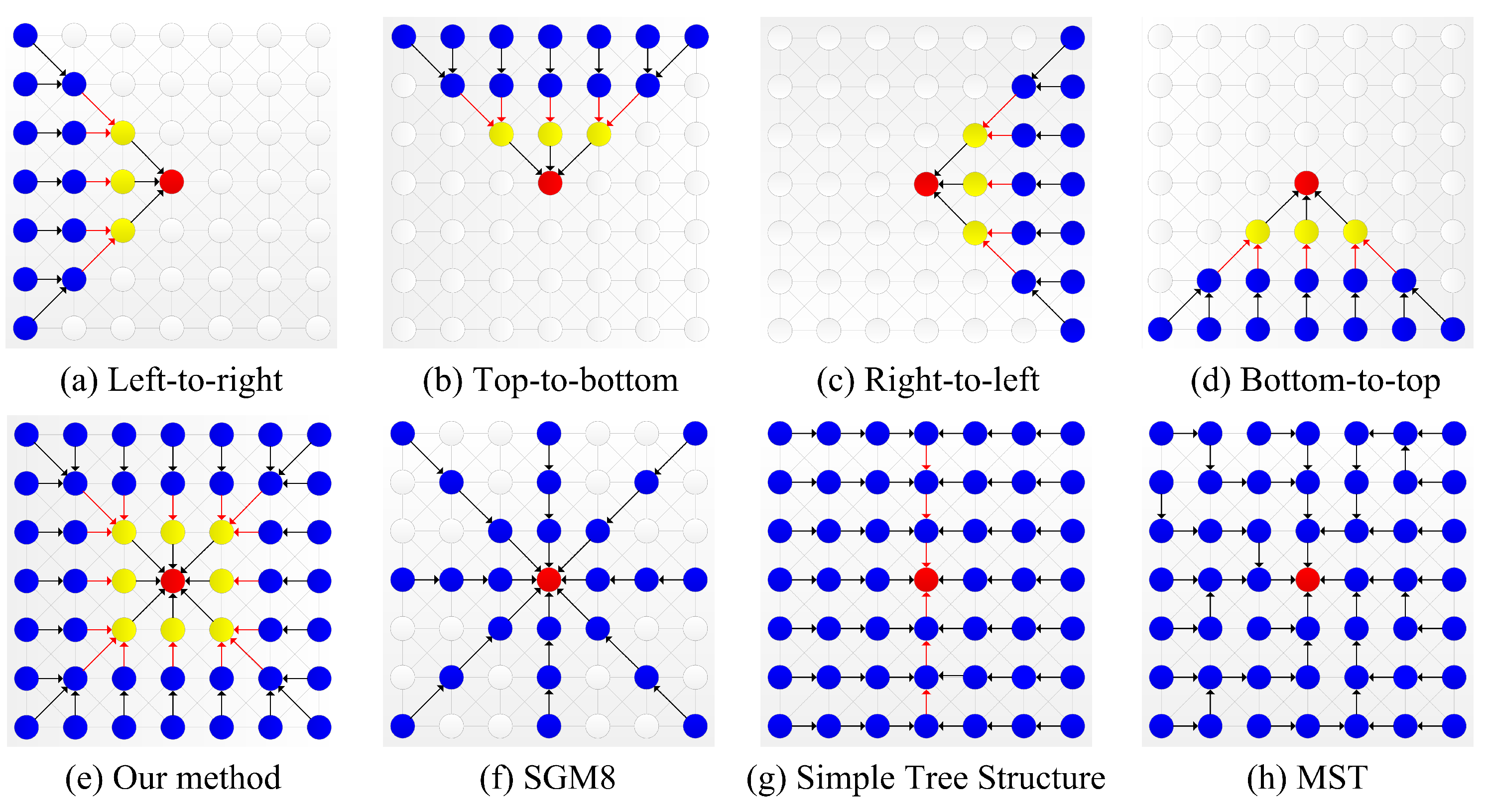
Figure 3e presents pixels contributing to the aggregated cost of root node in our method. We can see that root node gains supports from all pixels in the reference image and any pixel in the image contributes to the output of root node only once. Figure 3f–h illustrate the ways of information propagated in SGM variants. Figure 3f describes traditional SGM along eight directions. As explained in Ref. [30], two adjacent pixels are loosely related for that they only share the pixels on the same scan line. When matching costs on this line are weak, different disparities could be generated for multiple passes, resulting in streak artifacts in the disparity image. However, all pixels in the reference image contribute to the aggregated cost of root node, and a huge number of pixels are shared by neighboring root nodes, enhancing the reliability of aggregated cost in homogeneous area, since streak artifacts can be reduced in our result. Figure 3g shows the simple tree structure in Ref. [33]. The 1D optimization is performed along rows at first and then along columns. Although they utilized two tree structures which are complementary with each other, streak artifacts still appear in the disparity image. Figure 3h presents the minimum tree structure used in Ref. [34]. Neighboring pixels may have large distance on the MST, so that useful information cannot effectively propagate across the entire image, resulting in noisy disparity image.

2.3. Cost Volume Update Scheme

Although all pixels in the reference image are taken into account in our omni-directional SGM, it is still challenging to correctly recover disparities for pixels in large weakly textured area. Therefore, we use the output of previous pass to improve the robustness of initial matching cost. It is implemented by three steps: (1) an confidence map is built to evaluate the reliability of aggregated cost in last pass; (2) normalizing the aggregated costs to the same range as initial costs; (3) integrating normalized aggregated cost with initial matching cost based on the confidence of aggregated cost. These three steps are iteratively carried out until the last pass, enabling reliable information to propagate across the entire image.

We utilize the gap between the first minimum cost and the second minimum cost to define the confidence of aggregated cost for each pixel. Denote the first minimum cost and the second minimum cost as $L_{\mathit{r}}^{m1}$ and $L_{\mathit{r}}^{m2}$ respectively. For pixel $\mathit{p}$, we have:

$$\Gamma \left(\mathit{p}\right)=\frac{(L_{\mathit{r}}^{m2}\left(\mathit{p}\right)-L_{\mathit{r}}^{m1}\left(\mathit{p}\right))}{L_{\mathit{r}}^{m2}\left(\mathit{p}\right)+{\epsilon }_1}$$

(11)

where ${\epsilon }_1$ is a small number to avoid division by zero.

In order to normalize aggregated cost to the same range with initial cost volume, we first estimate the maximum of initial cost volume, $C_{max}^I$, the minimum and the maximum of aggregated cost for the last pass, $C_{min}^A$ and $C_{max}^A$, and then the normalized aggregated cost of pixel $\mathit{p}$ at disparity d in direction $\mathit{r}$ can be formulated by:

$$L_{\mathit{r}}^N(\mathit{p},d)=\frac{(L_{\mathit{r}}(\mathit{p},d)-C_{min}^A)\times C_{max}^I}{(C_{max}^A-C_{min}^A+{\epsilon }_2)}$$

(12)

where ${\epsilon }_2$ also is a small number, $L_{\mathit{r}}^N(\mathit{p},d)$ is the normalized cost of pixel $\mathit{p}$ at disparity d.

The cost update scheme is an adaptive combination of initial cost volume and the normalized aggregated cost in the previous pass. In order to inhibit the propagation of unreliable information, we introduce parameter $\omega$ to decide the ratio of two kind of costs in the updated cost volume. For pixel $\mathit{p}$ at disparity d, we have:

$$\begin{array}{cc}\hfill \phi \left(\mathit{p}\right)=& \min (\omega ·\zeta (\Gamma \left(\mathit{p}\right),\tau ),1.0)\hfill \end{array}$$

(13)

$$\begin{array}{cc}\hfill \overline{C}(\mathit{p},d)=& (1-\phi \left(\mathit{p}\right))C(\mathit{p},d)+\phi \left(\mathit{p}\right)·L_{\mathit{r}}^N(\mathit{p},d)\hfill \end{array}$$

(14)

where $\omega$ decides the amount of cost propagated to initial cost volume. $\zeta (\lambda ,\tau )$ is a truncation function which is $\lambda$ when $\lambda \ge \tau$, and 0 otherwise. $\tau$ is a threshold determining the cost of which pixel will be updated. Equation (13) decides the ratio of normalized aggregated cost for each pixel in updated cost volume. The min operation in Equation (13) indicates the ratio of normalized aggregated cost in the updated cost volume should be smaller than 1.0. When $\omega \approx 0$, then $\phi \left(\mathit{p}\right)$ is close to 0. This means that initial cost volume nearly remains the same in the aggregation procedures along multiple directions. When $\omega$ is a large number, we have $\phi \left(\mathit{p}\right)\approx 1.0$, which means we utilize the normalized aggregated cost as the input of next pass, it is similar to the strategy used in Ref. [33]. However, it will result in the wide spread of unreliable matching cost, deteriorating the quality of the disparity image.

With this cost volume update scheme, the formulas of our algorithm in each direction are slightly different from that provided in Section 2.2. The initial cost volume $C(\mathit{p},d)$ in Equations (6)–(8) should be replaced by $\overline{C}(\mathit{p},d)$. Suppose the size of input image is M×N, and the disparity space is D. Traditional SGM only takes the message from pixel on the same scan line into account, so that the computational complexity of traditional SGM is $O\left(MND\right)$. MGM utilizes the information from pixels visited in previous scan line, and the computational complexity of MGM is two times of that for SGM. Our method needs to compute the outputs from all three child nodes, since the computational complexity is three times of that for SGM. However, both SGM and our method can be implemented in parallel taking advantage of FPGA, while MGM can only be implemented in a raster order as it introduces dependency along the neighboring scan lines. A comparison of SGM, MGM and our method on computational complexity, parallelization, and pixels under consideration are presented in

Table 1. Comparison of SGM, MGM and our Omni-directional SGM.

Method	Computational Complexity	Parallelization	Pixels under Consideration
SGM [22]	O(MND)	Yes	Few
MGM [30]	O(MND)	No	All
Our method	O(MND)	Yes	All

. Our method takes pixels in the whole image into account with little extra computational cost, and still can be implemented in parallel.

2.4. Stable Disparity Propagate along MST

Disparity refinement is an extra step to further enhance the quality of disparity image. With disparity images of a stereo pair, left-right consistency check is used to divide all pixels into stable or unstable pixels. Various methods have been proposed to recover the disparities of mismatched pixels, such as plane fitting [12] and weighted median filter [5]. However, these methods only take pixels in local support window into account and are not geometric adaptive. Yang [15] proposed a non-local refinement method utilizing the MST of reference image. A new cost value is computed for each stable pixel at all candidate disparities, while it is 0 for unstable pixels. Then this cost volume is filtered by the non-local filter to propagate disparities of stable pixels to unstable pixels. Non-local refinement method is effective in many occasions, even when there are only few stable pixels in a region. However, it is time consuming to build and filter the new cost volume, especially for high-resolution stereo pairs with large label space.

Here we propose an effective and direct way to propagate disparities of stable pixels across the reference image making use of the MST, as shown in Figure 4. Similar to performing cost aggregation along the MST, our disparity propagation procedure is also implemented by traversing the MST in two sequential passes, namely from leaf nodes to root node and then from root node to leaf nodes. In the first pass, disparities of stable pixels are propagated from child nodes to their parent nodes, as shown in Figure 4a. Denote the parent node and child node of node v as $P\left(v\right)$ and $Ch\left(v\right)$, the weight of node v as $w\left(v\right)$. For an unstable pixel $\mathit{i}$, its disparity is decided by the most similar stable child node, which can be expressed by

$$D\left(\mathit{i}\right)=\left\{\begin{array}{cc}D\left(\mathit{p}\right)\hfill & \mathrm{if}w\left(\mathit{p}\right)=={\min }_{\mathit{q}\in Ch\left(i\right),\mathit{q}\in stable}\left(w\left(\mathit{q}\right)\right)\hfill \\ 0\hfill & \mathrm{else}\hfill \end{array}\right.$$

(15)

The cost of propagating disparity $D\left(\mathit{p}\right)$ to $D\left(\mathit{i}\right)$ is $c^{\uparrow }\left(\mathit{i}\right)$, and $c^{\uparrow }\left(\mathit{i}\right)=w\left(\mathit{p}\right)$. In the second pass, reliable disparities are propagated from from parent node to its child nodes, as shown in Figure 4b. For an unstable pixel $\mathit{i}$, its disparity is updated by

$$D\left(\mathit{i}\right)=\left\{\begin{array}{cc}D\left(P\right(i\left)\right)\hfill & \mathrm{if}{c}^{\uparrow }\left(\mathit{i}\right)\ge w\left(\mathit{i}\right)\hfill \\ D\left(i\right)\hfill & \mathrm{else}\hfill \end{array}\right.$$

(16)

From Equations (15) and (16), we can see that our method selects the disparity of the most similar stable pixel and propagates it to unstable pixel along the MST, and there is not much computational cost in the refinement step. Thus, our propagation strategy is more efficient than the non-local refinement approach [15]. Moreover, our method inherits the advantage of the non-local refinement approach to deal with huge unstable regions. In total, our strategy achieves similar performance to Yang’s method [15] but more efficient.

3. Experiments

In this section, we first give the parameter settings used in our experiments and then compare our approach with typical cost aggregation methods on widely used data sets, namely Middlebury dataset [9,35,36] and KITTI dataset [37,38], to demonstrate the effectiveness of our method.

3.1. Parameter Settings

There are six parameters in our omni-directional semi-global stereo matching framework, namely $P_1$ and $P_2$ for regularization in Equation (1), small constants ${\epsilon }_1$ and ${\epsilon }_2$ in Equations (11) and (12) to avoid division by zero, $\omega$ and $\tau$ in Equation (13) determine the ratio of normalized aggregated cost in updated cost volume. $P_1$, $P_2$ and $\omega$ are 0.01, 0.001, 0.3 for artificial indoor scenes and 1.0, 0.1, 0.5 for real world stereo images. $\tau$ is 0.5 in all data sets. Both ${\epsilon }_1$ and ${\epsilon }_2$ are 0.001 in all experiments. We use the default parameters in disparity refinement as in Ref. [15].

3.2. Middlebury Dataset

The Middlebury benchmark [9] provides a standard to compare different stereo matching algorithms. In the early datasets [35,39], stereo images are created under restricted conditions for indoor scenes with ground truth generated by structured light. Many approaches achieve quite satisfactory results on these stereo pairs. Therefore, they provide more challenging stereo pairs for natural real scenes with large low textural regions.

Stereo Pairs from Restricted Conditions: We use the four testing stereo images (Tsukuba, Venus, Cones, Teddy) used for evaluation on the benchmark and stereo images in both Middlebury 2005 and Middlebury 2006 datasets [9,35] to evaluate the performances of our method, SGM and its variants. As most of these stereo images contain rich texture, we adopt intensity + gradient to compute matching cost of corresponding pixels. For pixel $(i,j)$ at candidate disparity l, the matching cost can be formulated as

$$C_{i,j}\left(l\right)=(1-\lambda )·\min \left(\right||I_{i,j}-I_{i-l,j}^{{}^{\prime }}\left|\right|,{\tau }_1)+\lambda ·\min (\left|\right|{\nabla }_x{I}_{i,j}-{\nabla }_x{I}_{i-l,j}^{{}^{\prime }}\left|\right|,{\tau }_2)$$

(17)

Here, ${\nabla }_x$ is the gradient in x direction, $I_{i,j}$ and $I_{i-l,j}^{{}^{\prime }}$ are the color vectors of pixel $(i,j)$ and corresponding pixel $(i-l,j)$ in the other image. Parameter $\lambda$ balances the intensity term and the gradient term, and ${\tau }_1$, ${\tau }_2$ corresponds to the truncation values for these two terms, respectively. In our experiments, they are 0.89, 7/255 and 2/255 and remain the same in various methods. Then we perform optimization along each tree and fuse the outputs to obtain the aggregated cost. The initial disparity image is obtained by Equation (5).

Table 2. Percentages of error pixel (/%) in non-occluded region and corresponding rankings for typical cost aggregation methods on Middlebury dataset [9].

Method	BF	GF	NL	ST	MGM	SGM4	SGM8	Ours
Aloe	6.93${}_7$	5.29${}_6$	4.79${}_5$	4.79${}_5$	4.44${}_4$	4.29${}_3$	4.26${}_2$	4.19${}_1$
Baby1	4.26${}_7$	3.62${}_5$	7.47${}_8$	4.10${}_6$	2.65${}_2$	2.84${}_4$	2.67${}_3$	2.33${}_1$
Baby2	3.47${}_5$	3.39${}_4$	11.94${}_7$	13.36${}_8$	1.87${}_1$	4.03${}_6$	2.54${}_3$	2.38${}_2$
Baby3	4.47${}_4$	3.98${}_2$	5.00${}_6$	4.29${}_3$	4.50${}_5$	5.42${}_8$	5.23${}_7$	3.18${}_1$
Bowling1	10.38${}_3$	9.36${}_2$	19.49${}_8$	19.44${}_7$	11.20${}_4$	13.64${}_5$	14.79${}_6$	7.56${}_1$
Bowling2	5.84${}_5$	4.70${}_2$	8.21${}_6$	8.25${}_7$	8.38${}_8$	4.89${}_4$	4.78${}_3$	3.37${}_1$
Cloth1	3.19${}_8$	1.20${}_7$	0.62${}_1$	0.63${}_2$	0.96${}_5$	0.73${}_4$	0.67${}_3$	1.15${}_6$
Cloth2	6.11${}_8$	1.89${}_1$	3.87${}_6$	3.74${}_5$	2.25${}_2$	2.47${}_3$	4.29${}_7$	2.75${}_4$
Cloth3	3.39${}_8$	1.70${}_1$	2.39${}_6$	2.57${}_7$	1.92${}_2$	2.09${}_4$	2.06${}_3$	2.35${}_5$
Cloth4	3.23${}_8$	2.92${}_7$	1.81${}_2$	1.80${}_1$	1.97${}_3$	1.99${}_4$	2.00${}_5$	2.21${}_6$
Flowerpots	8.33${}_4$	7.52${}_2$	13.56${}_8$	10.13${}_5$	7.42${}_1$	12.17${}_7$	11.21${}_6$	7.84${}_3$
Lampshade1	9.36${}_8$	7.81${}_4$	8.64${}_5$	9.23${}_6$	6.29${}_2$	9.37${}_7$	6.58${}_3$	4.85${}_1$
Lampshade2	17.11${}_8$	16.42${}_7$	11.80${}_6$	11.56${}_5$	8.57${}_2$	9.80${}_4$	8.80${}_3$	6.49${}_1$
Rocks1	5.05${}_8$	2.75${}_7$	2.50${}_6$	2.42${}_5$	1.75${}_3$	1.73${}_2$	1.65${}_1$	1.96${}_4$
Rocks2	4.78${}_8$	1.21${}_1$	1.70${}_7$	1.67${}_6$	1.37${}_2$	1.64${}_5$	1.59${}_4$	1.50${}_3$
Wood1	5.55${}_7$	3.22${}_4$	8.49${}_8$	4.41${}_6$	4.38${}_5$	1.47${}_1$	1.82${}_3$	1.73${}_2$
Wood2	1.91${}_4$	1.38${}_3$	2.05${}_5$	2.57${}_7$	1.33${}_2$	2.27${}_6$	3.04${}_8$	1.29${}_1$
Art	8.89${}_6$	8.00${}_2$	9.13${}_8$	9.03${}_7$	8.79${}_5$	8.03${}_3$	8.12${}_4$	6.17${}_1$
Books	11.60${}_8$	8.80${}_4$	10.44${}_7$	10.01${}_6$	8.95${}_5$	8.30${}_3$	8.10${}_2$	6.92${}_1$
Cones	4.37${}_5$	2.33${}_1$	3.53${}_2$	3.83${}_3$	5.36${}_8$	4.70${}_7$	4.64${}_6$	3.78${}_4$
Dolls	6.15${}_8$	4.15${}_2$	4.97${}_5$	4.51${}_4$	3.94${}_1$	5.25${}_7$	5.10${}_6$	4.22${}_3$
Laundry	12.21${}_5$	11.31${}_3$	10.46${}_2$	10.42${}_1$	15.59${}_7$	15.60${}_8$	15.10${}_6$	11.70${}_4$
Moebius	9.77${}_8$	8.35${}_4$	7.52${}_3$	7.37${}_2$	8.76${}_5$	9.66${}_6$	9.67${}_7$	7.20${}_1$
Reindeer	8.93${}_7$	6.26${}_5$	9.50${}_8$	7.55${}_6$	5.41${}_2$	6.94${}_3$	6.69${}_4$	4.90${}_1$
Teddy	7.30${}_6$	6.35${}_3$	5.17${}_1$	5.64${}_2$	9.51${}_8$	7.28${}_5$	7.41${}_7$	6.62${}_4$
Tsukuba	2.34${}_5$	2.30${}_4$	1.76${}_2$	2.04${}_3$	2.53${}_6$	2.58${}_7$	2.34${}_5$	1.48${}_1$
Venus	0.83${}_4$	0.64${}_2$	0.61${}_1$	0.76${}_3$	1.27${}_8$	1.14${}_7$	1.10${}_6$	1.07${}_5$
Average	6.51${}_{6.4}$	5.07${}_{3.5}$	6.57${}_{5.2}$	6.15${}_{4.7}$	5.24${}_{4.0}$	5.56${}_{4.9}$	5.42${}_{4.6}$	4.10${}_{2.5}$

presents the percentage of error pixel in non-occluded region and corresponding rankings for kinds of cost aggregation methods. Our method achieves the smallest average error rate and ranks the first among these approaches. BF and GF are local methods which aggregate costs in a local support window, since they generate high quality disparity images for stereo pairs containing a lot of details, such as Cones and Rocks2. GF attempts to preserve the structure of reference image in the filtering result, since GF shows better edge-preserving property than BF and achieves lower error rate. NL and ST are tree-based filtering approaches which aggregate cost in the whole image by recursively traversing the tree in two passes. Although all pixels are taken into account, they only use intensity difference to estimate the similarity of any two pixels on the tree and tend to overuse smooth constraint in low textural area, resulting in an increase of error rate. SGM and its variants, including our method, incorporate information from multiple directions and produce more accurate disparity image.

Table 3. Comparison with state-of-the-art non-local cost aggregation approaches on Middlebury dataset [9]. O_all: percentage of erroneous pixels in all region. O_noc: percentage of erroneous pixels in non-occluded region.

Method	Initial Disparity		Final Disparity
	O_noc	O_all	O_noc	O_all
NL [7]	6.57%	17.20%	6.64%	12.67%
ST [16]	6.15%	17.34%	6.27%	12.30%
SGM4 [22]	5.56%	18.34%	4.59%	11.05%
SGM8 [22]	5.42%	18.17%	4.78%	11.21%
MGM [30]	5.24%	17.62%	4.47%	11.21%
Our method	4.10%	17.43%	3.71%	10.57%

lists average error rates of several non-local cost aggregation methods. We can see that our method outperforms other approaches in most metrics. The error rate of SGM8 is lower than that of SGM4 for the initial disparity image. The reason for this is that SGM8 propagates information along eight directions; thus, reliable information can propagate into occluded and weakly textured regions to deal with the ambiguity of these pixels. However, the error rates of final disparity image for SGM4 is lower than that of SGM8. One reason for this is that most of these stereo pairs are high texture images, so that aggregated costs along four directions are robust enough to generate accurate disparity image for these stereo pairs. Another reason is that streak artifacts in the results of SGM8 are more severe than that of SGM4. MGM performs better than SGM4 and SGM8 because there are multiple paths between any two pixels, which strengthens the interactions of pixels in the local region.

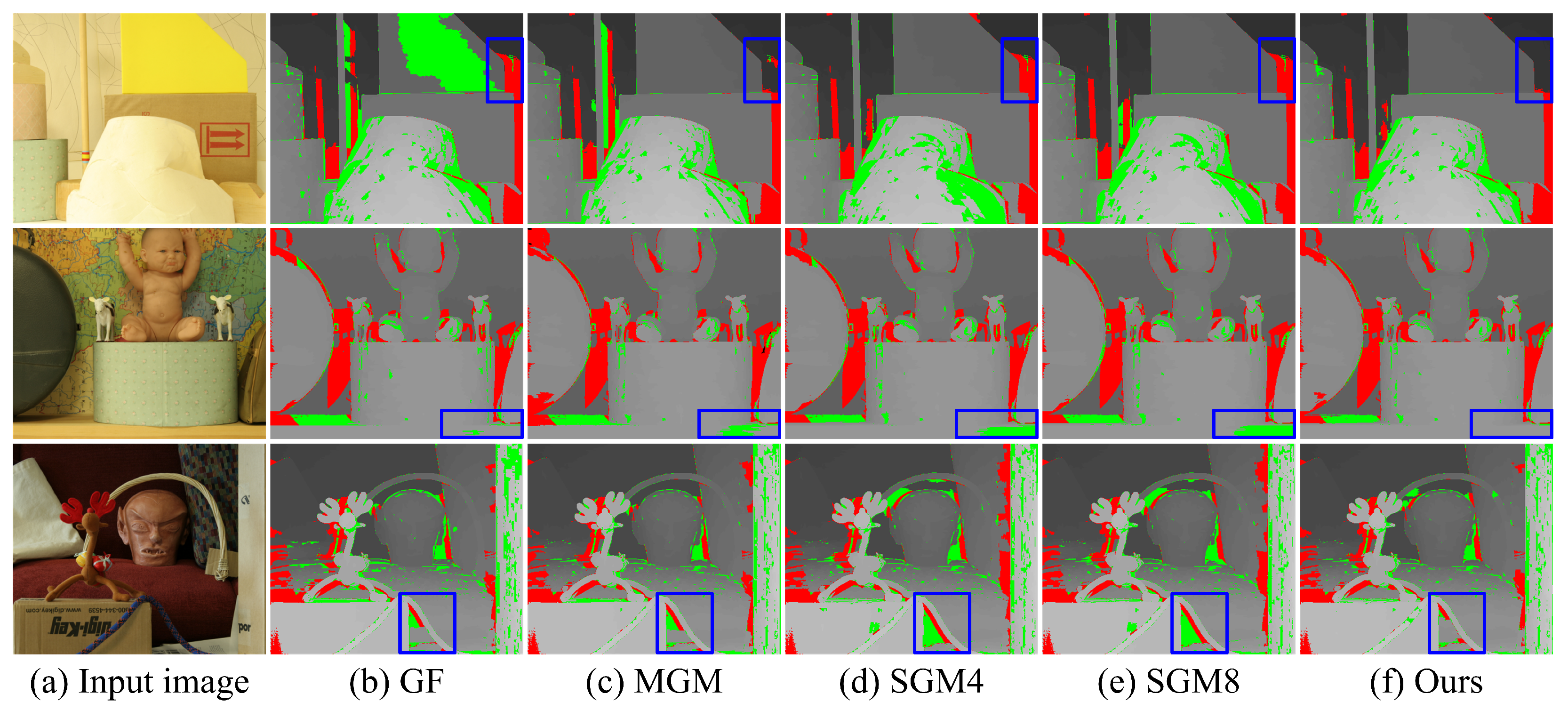
After disparity refinement, our OmniSGM achieves the best results among these approaches. The error rates for non-occluded and all regions for final disparity image are decreased by 0.87% and 0.63% respectively, when compared with that of SGM8. The performance of ST and NL is inferior to those SGM-based methods for the overusing of piece-wise constant assumption. Figure 5 shows examples of disparity images for GF, SGM, MGM and our method. Our method generates better results than GF, SGM, and MGM. Disparities of all major structures are correctly predicted and reliable disparities propagate along the MST to recover that of unstable pixels. GF utilizes information in a local window, and SGM only takes pixels on multiple scan lines into account, so that neither of them can effectively solve the ambiguity in the low textural area. Our method incorporates useful information from pixels in the whole image and successively improves the robustness of initial cost volume, since we achieve the best results among these methods.

Stereo Pairs from Natural Conditions: Middlebury 2014 dataset [36] provides high-resolution stereo pairs with large label space under natural conditions. The 10 testing stereo pairs with ground truth are used to evaluate the effectiveness of typical cost aggregation methods. Here, we use Census Transform (CT) in a 9 × 9 window to compute matching cost, and normalize the matching cost to [0, 1.0] to avoid tremendous message. In order to fairly compare various cost aggregation methods, we perform evaluation of average error rate and average endpoint error for initial disparity images.

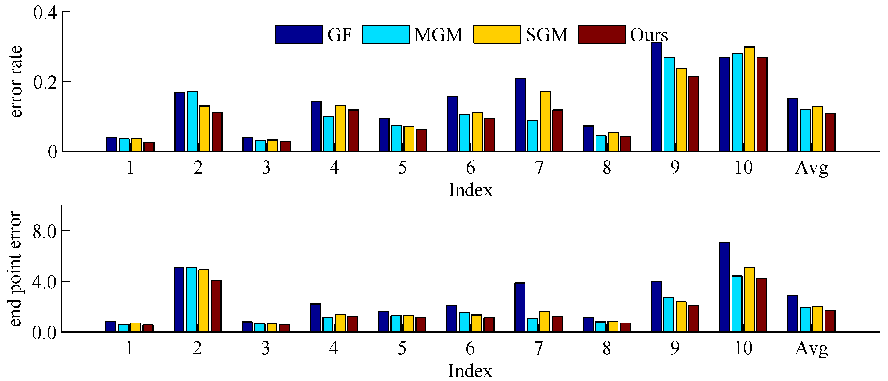
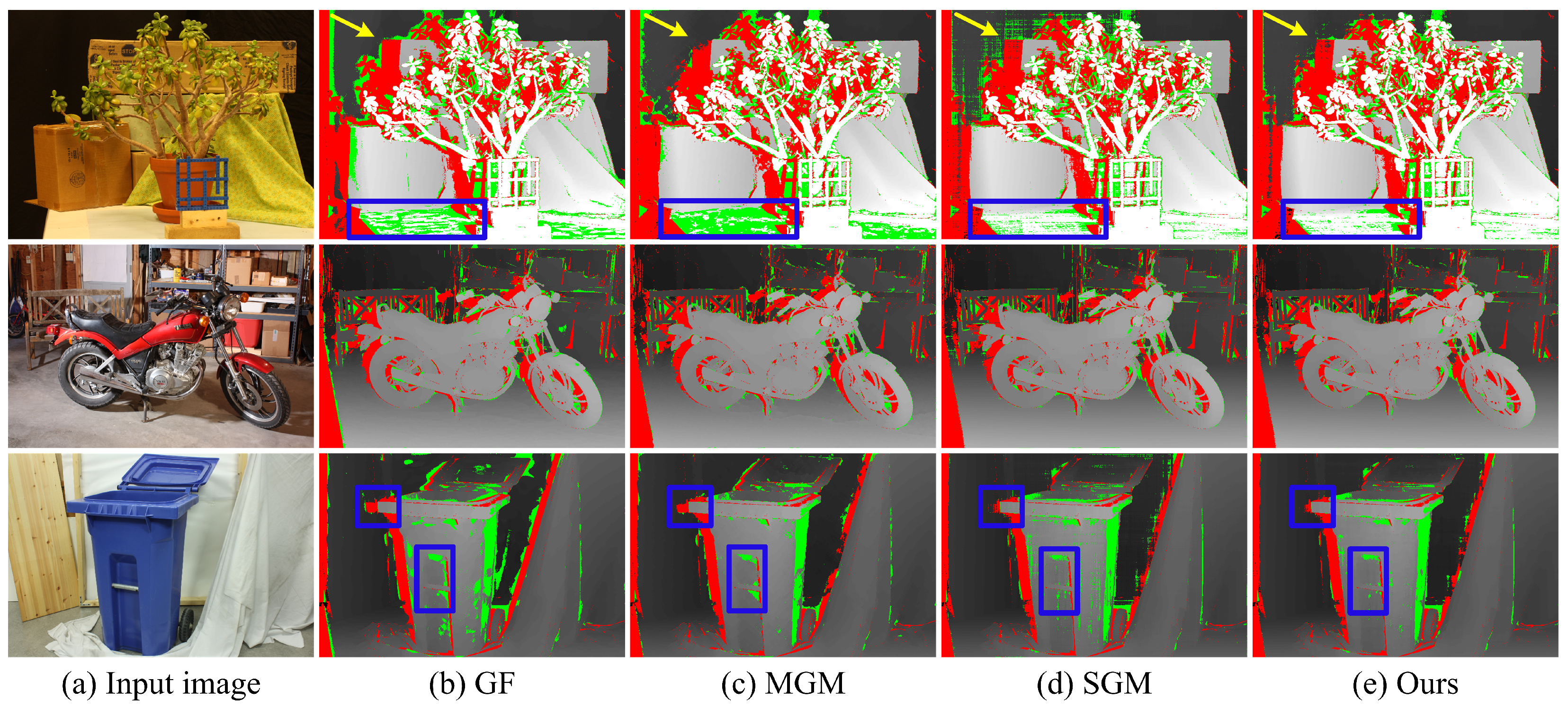
Figure 6 shows the error rate and endpoint error of testing stereo pairs for GF, SGM, MGM and our method. We can see that our method outperforms GF, SGM and MGM almost on all testing images in both metrics. The superiority of our method is more obvious on stereo pairs with large weakly textured area, such as the second and the ninth testing images. The accuracy gains come from our omni-directional SGM tries to aggregate information from all pixels along all directions and the successive cost volume update scheme. GF incorporates costs in a local window to suppress noise. However, most stereo pairs in this dataset contain large low textural area, since merely taking pixels in a local window into account cannot solve the ambiguity in these areas, resulting in the worst performance among these methods. MGM produces poor results for testing images with large weakly textured regions as it enforces strong local smoothness constraint which inhibits informative messages from being propagated in wide range. Figure 7 presents examples of disparity images for GF, SGM, MGM and our method. It can be seen that our method generates high quality disparity images on these challenging stereo pairs. Our method successfully recovers the disparities of pixels not only in major structures and fine-scale details, but also in large homogeneous area, such as ground.

3.3. KITTI Dataset

KITTI dataset [37,38] provides real-world testing images with street views taken from a driving car, and most of the images in the dataset contain large portion of homogeneous regions, such as walls and roads. Considering illumination difference and large challenging areas, we adopt two ways to build initial cost volume, namely CT and the correlation of feature maps from PSMNet [40].

KITTI 2012 Dataset:

Table 4. Comparison with state-of-the-art cost aggregation approaches on KITTI 2012 dataset [37]. O_all: percentage of erroneous pixels in all region (/%). O_noc: percentage of erroneous pixels in the non-occluded region (/%). A_all: average disparity error in all region (/px). A_noc: average disparity error in the non-occluded region (/px). “/”: the results are not available.

Method	Initial Disparity				Final Disparity
	O_all	A_all	O_noc	A_noc	O_all	A_all	O_noc	A_noc
NL [15]	13.87	3.80	11.67	2.45	11.57	1.97	10.26	1.75
ST [16]	15.66	3.86	13.50	2.53	13.44	2.15	12.16	1.93
SGM [22]	/	/	/	/	9.13	2.00	7.64	1.80
LDESGM [41]	/	/	/	/	8.22	2.40	6.01	1.40
iSGM [24]	/	/	/	/	7.15	2.10	5.11	1.20
wSGM [42]	/	/	/	/	6.18	1.60	4.97	1.30
MGM [30]	12.03	3.10	9.84	2.00	11.02	2.59	8.77	1.61
LRNL [18]	9.29	2.88	7.49	2.00	8.51	2.07	7.14	1.67
Our_Feat	7.52	2.59	5.24	1.49	6.83	2.24	4.49	1.29
Our_Cen	8.45	2.52	6.14	1.37	6.42	1.57	4.96	1.16

presents the results of various non-local cost aggregation approaches. Both NL and ST treat reference image as undirected graph and extract the MST by removing edges with large gradients. These two methods tend to overuse piece-wise constant assumption, leading to producing poor results. LDESGM [41] proposes a new local binary encoding pattern based on the intensity relationship between pixels in horizontal, vertical and diagonal directions, and combines this metric with magnitude information to solidify matching cost, then adopts SGM in eight directions to aggregate cost. Our method outperforms LDESGM with a great margin on both metrics, and the average error rates in non-occluded and all regions are reduced by 1.05% and 1.52% respectively. Compare with MGM, the average errors in all and non-occluded regions of our method using CT to compute matching cost are decreased by 1.02 px and 0.45 px respectively. iSGM [24] iteratively evaluates accumulated cost and intermediate disparity images in scale space to guide the cost aggregation in next pass. Although simpler scheme used in our method, we achieve lower error rate and average disparity error in all region. The gains of iSGM and wSGM mainly stem from coarse-to-fine strategy, complicate cost function, multiple refinement steps and subsidiary information.

Compare the results of our method using different features to build cost volume, learning-based features generate lower error rate while census transform has smaller average disparity error. This isbecause learning-based features with a large receptive field can reason about local geometry using a wide range of textural information, making these features more robust in a homogeneous area. A handcrafted feature is more accurate than learning-based features to evaluate the similarity of corresponding pixels in high texture regions. We intend to combine the superiority of these two features in building cost volume. Specifically, using a handcrafted feature in a highly textured area preserves fine-scale details and adopting learning-based features in a homogeneous region reduces ambiguity. We will work on this in the future.

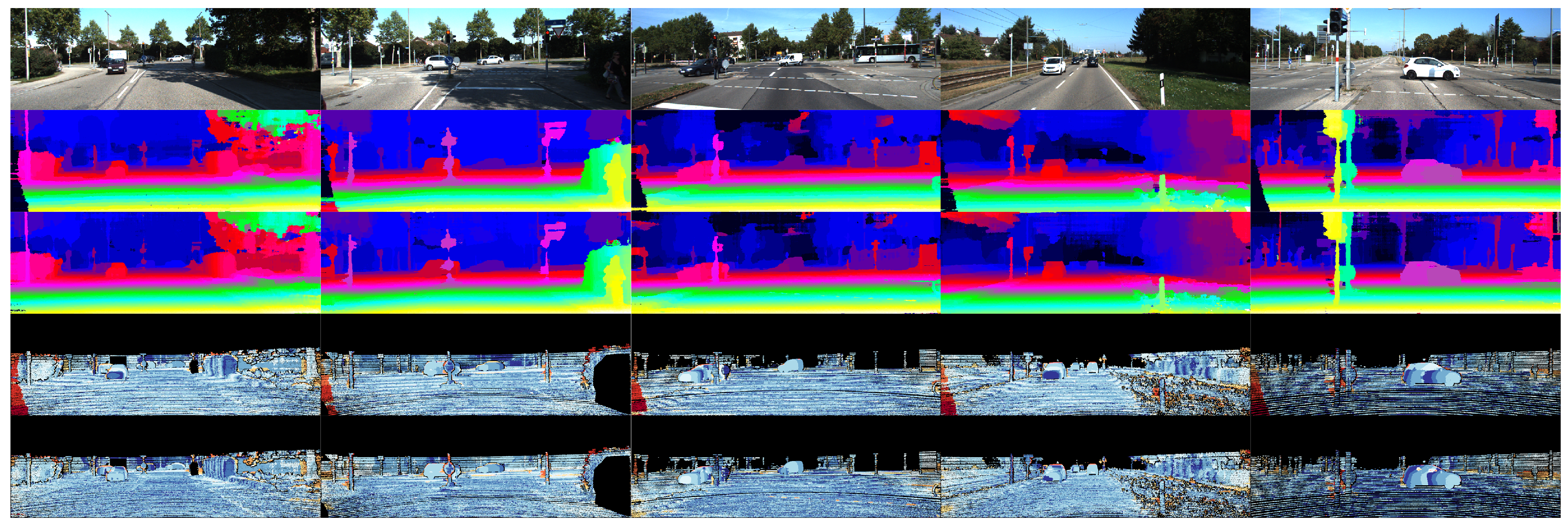
Figure 8 shows some results of our method on KITTI 2012 dataset [37]. We can see that our approach produces satisfactory disparity images using both features to compute matching cost. Most of the erroneous pixels are located in image borders for disparity images generated by learning-based features, while large errors are in weakly textured areas when using handcrafted feature to compute matching cost.

KITTI 2015 Dataset:

Table 5. Comparison of typical cost aggregation methods on KITTI 2015 dataset [38].

Method	Initial Disparity				Final Disparity
	O_all	A_all	O_noc	A_noc	O_all	A_all	O_noc	A_noc
NL [15]	11.30	2.57	10.09	2.11	8.91	1.66	8.61	1.64
ST [16]	12.57	2.68	11.37	2.22	9.97	1.74	9.68	1.72
SGM [22]	/	/	/	/	10.86	/	8.92	/
SFSGM [43]	/	/	/	/	13.37	/	11.93	/
MFSGM [28]	/	/	/	/	8.24	/	6.91	/
MGM [30]	13.17	2.57	12.01	2.15	11.79	2.40	10.66	1.92
LRNL [18]	7.79	2.29	7.06	2.05	6.35	1.55	6.13	1.53
Our_Feat	8.07	2.07	6.88	1.65	6.90	1.78	5.74	1.43
Our_Cen	8.09	1.92	6.85	1.50	5.88	1.30	5.55	1.25

lists the results of state-of-the-art non-local cost aggregation methods on KITTI 2015 dataset. Similar to that in KITTI 2012 dataset, NL and ST generate poor disparity images for overusing of piece-wise constant assumption. SFSGM extends 2D motion information to 3D space by combining stereo matching with optical flow estimation, while the error rates for their method are nearly twice of that for ours. A variant of CT, named Center-Symmetric Census Transform (CSCT), is adopted in MFSGM to improve the performance of SGM. The error rates of our method using CT in all and non-occluded regions are 5.88% and 5.55%, which are lower than that of MFSGM by 2.36% and 1.36%. Our method outperforms MGM in all metrics. Figure 9 presents the results from the KITTI 2015 dataset. Disparities in large homogeneous regions are successfully predicted, as well as that of complicated geometric structures, such as poles and cars. Most erroneous pixels still lie in the image borders. The reason for this is that these outdoor stereo pairs contain large slant surfaces, and the disparities of pixels in these regions cannot be determined by the propagation of disparities from stable pixels. It is necessary to adopt a more sophisticated refinement approach, such as segmentation and plant fitting.

4. Conclusions and Remarks

In this paper, we present a novel omni-directional semi-global stereo matching framework. Messages propagate along all directions and each pixel obtains support from pixels in the whole image. The contribution of each pixel can be computed recursively along the tree structures. Specifically, we divide the entire image into four parts and compute the contributions of pixels on four tree structures, namely trees in the left, right, top, and bottom of root node, and then fuse the results to obtain contributions from pixels in the whole image. We also propose a cost volume update scheme to enhance the robustness of initial cost volume, since the quality of disparity image can be improved in the following pass. Finally, an efficient stable disparity propagation strategy along the MST is presented for disparity refinement.

We validate the effectiveness of our method on challenging datasets, and find that a stereo matching algorithm can benefit from the combination of handcrafted feature and feature maps from CNN, as they own the merits to deal with pixels in different regions. We will work on this in the future.

References

1. Caetano, F.; Carvalho, P.; Cardoso, J. Deep Anomaly Detection for In-Vehicle Monitoring—An Application-Oriented Review. Appl. Sci. 2022, 12, 10011. [Google Scholar] [CrossRef]
2. Shehzadi, T.; Hashmi, K.A.; Pagani, A.; Liwicki, M.; Stricker, D.; Afzal, M.Z. Mask-Aware Semi-Supervised Object Detection in Floor Plans. Appl. Sci. 2022, 12, 9398. [Google Scholar] [CrossRef]
3. Xu, B.; Sun, Y.; Meng, X.; Liu, Z.; Li, W. MreNet: A Vision Transformer Network for Estimating Room Layouts from a Single RGB Panorama. Appl. Sci. 2022, 12, 9696. [Google Scholar] [CrossRef]
4. Zhang, K.; Fang, Y.; Min, D.; Sun, L.; Yang, S.; Yan, S.; Tian, Q. Cross-scale cost aggregation for stereo matching. In Proceedings of the IEEE Conference on Computer Vision and Pattern Recognition, Columbus, OH, USA, 23–28 June 2014; pp. 1590–1597. [Google Scholar]
5. Hosni, A.; Rhemann, C.; Bleyer, M.; Rother, C.; Gelautz, M. Fast Cost-Volume Filtering for Visual Correspondence and Beyond. IEEE Trans. Pattern Anal. Mach. Intell. 2013, 35, 504–511. [Google Scholar] [CrossRef] [PubMed]
6. Tan, X.; Sun, C.; Wang, D.; Guo, Y.; Pham, T.D. Soft cost aggregation with multi-resolution fusion. In Proceedings of the European Conference on Computer Vision, Zurich, Switzerland, 6–12 September 2014; Springer: Berlin/Heidelberg, Germany, 2014; pp. 17–32. [Google Scholar]
7. Yang, Q. Stereo Matching Using Tree Filtering. IEEE Trans. Pattern Anal. Mach. Intell. 2015, 37, 834–846. [Google Scholar] [CrossRef] [PubMed]
8. Lu, J.; Shi, K.; Min, D.; Lin, L.; Do, M.N. Cross-based local multipoint filtering. In Proceedings of the 2012 IEEE Conference on Computer Vision and Pattern Recognition, Providence, RI, USA, 16–21 June 2012; pp. 430–437. [Google Scholar]
9. Scharstein, D.; Szeliski, R. A taxonomy and evaluation of dense two-frame stereo correspondence algorithms. Int. J. Comput. Vis. 2002, 47, 7–42. [Google Scholar] [CrossRef]
10. Taniai, T.; Matsushita, Y.; Sato, Y.; Naemura, T. Continuous 3D label stereo matching using local expansion moves. IEEE Trans. Pattern Anal. Mach. Intell. 2017, 40, 2725–2739. [Google Scholar] [CrossRef] [Green Version]
11. Kwatra, V.; Schödl, A.; Essa, I.; Turk, G.; Bobick, A. Graphcut textures: Image and video synthesis using graph cuts. ACM Trans. Graph. ToG 2003, 22, 277–286. [Google Scholar] [CrossRef]
12. Yang, Q.; Wang, L.; Yang, R.; Stewénius, H.; Nistér, D. Stereo matching with color-weighted correlation, hierarchical belief propagation, and occlusion handling. IEEE Trans. Pattern Anal. Mach. Intell. 2008, 31, 492–504. [Google Scholar] [CrossRef] [PubMed]
13. Yoon, K.J.; Kweon, I.S. Adaptive support-weight approach for correspondence search. IEEE Trans. Pattern Anal. Mach. Intell. 2006, 28, 650–656. [Google Scholar] [CrossRef] [PubMed]
14. He, K.; Sun, J.; Tang, X. Guided image filtering. IEEE Trans. Pattern Anal. Mach. Intell. 2012, 35, 1397–1409. [Google Scholar] [CrossRef] [PubMed]
15. Yang, Q. A non-local cost aggregation method for stereo matching. In Proceedings of the 2012 IEEE Conference on Computer Vision and Pattern Recognition, Providence, RI, USA, 16–21 June 2012; pp. 1402–1409. [Google Scholar]
16. Mei, X.; Sun, X.; Dong, W.; Wang, H.; Zhang, X. Segment-tree based cost aggregation for stereo matching. In Proceedings of the IEEE Conference on Computer Vision and Pattern Recognition, Portland, OR, USA, 23–28 June 2013; pp. 313–320. [Google Scholar]
17. Achanta, R.; Shaji, A.; Smith, K.; Lucchi, A.; Fua, P.; Süsstrunk, S. SLIC superpixels compared to state-of-the-art superpixel methods. IEEE Trans. Pattern Anal. Mach. Intell. 2012, 34, 2274–2282. [Google Scholar] [CrossRef] [PubMed] [Green Version]
18. Bu, P.; Zhao, H.; Jin, Y.; Ma, Y. Linear Recursive Non-Local Edge-Aware Filter. IEEE Trans. Circuits Syst. Video Technol. 2020, 31, 1751–1763. [Google Scholar] [CrossRef]
19. Boykov, Y.; Kolmogorov, V. An experimental comparison of min-cut/max- flow algorithms for energy minimization in vision. IEEE Trans. Pattern Anal. Mach. Intell. 2004, 26, 1124–1137. [Google Scholar] [CrossRef] [PubMed] [Green Version]
20. Szeliski, R.; Zabih, R.; Scharstein, D.; Veksler, O.; Kolmogorov, V.; Agarwala, A.; Tappen, M.; Rother, C. A comparative study of energy minimization methods for markov random fields with smoothness-based priors. IEEE Trans. Pattern Anal. Mach. Intell. 2008, 30, 1068–1080. [Google Scholar] [CrossRef] [Green Version]
21. Felzenszwalb, P.F.; Huttenlocher, D.P. Efficient belief propagation for early vision. Int. J. Comput. Vis. 2006, 70, 41–54. [Google Scholar] [CrossRef]
22. Hirschmuller, H. Stereo Processing by Semiglobal Matching and Mutual Information. IEEE Trans. Pattern Anal. Mach. Intell. 2008, 30, 328–341. [Google Scholar] [CrossRef] [PubMed]
23. Gehrig, S.K.; Eberli, F.; Meyer, T. A real-time low-power stereo vision engine using semi-global matching. In Proceedings of the International Conference on Computer Vision Systems, Liège, Belgium, 13–15 October 2009; Springer: Berlin/Heidelberg, Germany, 2009; pp. 134–143. [Google Scholar]
24. Hermann, S.; Klette, R. Iterative semi-global matching for robust driver assistance systems. In Proceedings of the Asian Conference on Computer Vision, Daejeon, Korea, 5–9 November 2012; Springer: Berlin/Heidelberg, Germany, 2012; pp. 465–478. [Google Scholar]
25. Michael, M.; Salmen, J.; Stallkamp, J.; Schlipsing, M. Real-time stereo vision: Optimizing semi-global matching. In Proceedings of the 2013 IEEE Intelligent Vehicles Symposium (IV), Gold Coast, QLD, Australia, 23–26 June 2013; pp. 1197–1202. [Google Scholar]
26. Rahnama, O.; Cavalleri, T.; Golodetz, S.; Walker, S.; Torr, P. R3sgm: Real-time raster-respecting semi-global matching for power-constrained systems. In Proceedings of the 2018 International Conference on Field-Programmable Technology (FPT), Naha, Japan, 10–14 December 2018; pp. 102–109. [Google Scholar]
27. Steinbrücker, F.; Pock, T.; Cremers, D. Large displacement optical flow computation withoutwarping. In Proceedings of the 2009 IEEE 12th International Conference on Computer Vision, Kyoto, Japan, 29 September–2 October 2009; pp. 1609–1614. [Google Scholar]
28. Hernandez-Juarez, D.; Chacón, A.; Espinosa, A.; Vázquez, D.; Moure, J.C.; López, A.M. Embedded real-time stereo estimation via semi-global matching on the GPU. Procedia Comput. Sci. 2016, 80, 143–153. [Google Scholar] [CrossRef] [Green Version]
29. Schonberger, J.L.; Sinha, S.N.; Pollefeys, M. Learning to fuse proposals from multiple scanline optimizations in semi-global matching. In Proceedings of the European Conference on Computer Vision (ECCV), Munich, Germany, 8–14 September 2018; pp. 739–755. [Google Scholar]
30. Facciolo, G.; De Franchis, C.; Meinhardt, E. MGM: A significantly more global matching for stereovision. In Proceedings of the BMVC 2015, Swansea, UK, 7–10 September 2015. [Google Scholar]
31. Kallwies, J.; Engler, T.; Forkel, B.; Wuensche, H.J. Triple-SGM: Stereo Processing using Semi-Global Matching with Cost Fusion. In Proceedings of the IEEE/CVF Winter Conference on Applications of Computer Vision, Pitkin, CO, USA, 1–5 March 2020; pp. 192–200. [Google Scholar]
32. Seki, A.; Pollefeys, M. SGM-Nets: Semi-Global Matching with Neural Networks. In Proceedings of the IEEE Conference on Computer Vision and Pattern Recognition (CVPR), Honolulu, HI, USA, 21–26 July 2017; pp. 6640–6649. [Google Scholar]
33. Bleyer, M.; Gelautz, M. Simple but effective tree structures for dynamic programming-based stereo matching. In Proceedings of the International Conference on Computer Vision Theory and Applications, Funchal, Portugal, 22–25 January 2008; Volume 2, pp. 415–422. [Google Scholar]
34. Veksler, O. Stereo correspondence by dynamic programming on a tree. In Proceedings of the 2005 IEEE Computer Society Conference on Computer Vision and Pattern Recognition (CVPR’05), San Diego, CA, USA, 20–25 June 2005; Volume 2, pp. 384–390. [Google Scholar]
35. Scharstein, D.; Szeliski, R. High-accuracy stereo depth maps using structured light. In Proceedings of the 2003 IEEE Computer Society Conference on Computer Vision and Pattern Recognition, Madison, WI, USA, 18–20 June 2003; Volume 1, pp. 195–202. [Google Scholar]
36. Scharstein, D.; Hirschmüller, H.; Kitajima, Y.; Krathwohl, G.; Nešić, N.; Wang, X.; Westling, P. High-resolution stereo datasets with subpixel-accurate ground truth. In Proceedings of the German Conference on Pattern Recognition, Münster, Germany, 2–5 September 2014; Springer: Berlin/Heidelberg, Germany, 2014; pp. 31–42. [Google Scholar]
37. Geiger, A.; Lenz, P.; Urtasun, R. Are we ready for autonomous driving? The kitti vision benchmark suite. In Proceedings of the 2012 IEEE Conference on Computer Vision and Pattern Recognition, Providence, RI, USA, 16–21 June 2012; pp. 3354–3361. [Google Scholar]
38. Menze, M.; Geiger, A. Object scene flow for autonomous vehicles. In Proceedings of the IEEE Conference on Computer Vision and Pattern Recognition, Boston, MA, USA, 7–12 June 2015; pp. 3061–3070. [Google Scholar]
39. Scharstein, D.; Pal, C. Learning conditional random fields for stereo. In Proceedings of the 2007 IEEE Conference on Computer Vision and Pattern Recognition, Minneapolis, MN, USA, 17–22 June 2007; pp. 1–8. [Google Scholar]
40. Chang, J.R.; Chen, Y.S. Pyramid stereo matching network. In Proceedings of the IEEE Conference on Computer Vision and Pattern Recognition, Salt Lake City, UT, USA, 18–23 June 2018; pp. 5410–5418. [Google Scholar]
41. Nguyen, V.D.; Nguyen, D.D.; Lee, S.; Jeon, J.W. Local Density Encoding for Robust Stereo Matching. IEEE Trans. Circuits Syst. Video Technol. 2014, 24, 2049–2062. [Google Scholar] [CrossRef]
42. Spangenberg, R.; Langner, T.; Rojas, R. Weighted semi-global matching and center-symmetric census transform for robust driver assistance. In Proceedings of the International Conference on Computer Analysis of Images and Patterns, York, UK, 27–29 August 2013; Springer: Berlin/Heidelberg, Germany, 2013; pp. 34–41. [Google Scholar]
43. Schuster, R.; Bailer, C.; Wasenmuller, O.; Stricker, D. Combining Stereo Disparity and Optical Flow for Basic Scene Flow. In Proceedings of the 5th Commercial Vehicle Technology Symposium, Berlin, Germany, 13–15 March 2018; pp. 90–101. [Google Scholar]
Figure 1. Message propagation strategies and the results on Adirondack stereo images of SGM, MGM and our proposed OmniSGM in four directions (from top to bottom). Black line and red line indicate the directions of how message is propagated and the cost volume update scheme respectively. Black boxes in error maps show that our method and MGM successfully avoid streak artifacts in disparity image, and red boxes demonstrate that our result is more accurate result than that of MGM and SGM.
Applsci 12 11934 g001
Figure 2. Directions of information propagation on each tree structure. Red node is the root node, and orange nodes are children nodes.
Applsci 12 11934 g002
Figure 3. Message propagation strategies in SGM variants. (ad) show the ways to compute aggregated costs of root node along each tree in our method. The output of root node in each direction can be computed directly from the outputs of its children nodes (red lines). (e) Pixels contributing the output of root node in our method. (d) Pixels contributing to the output of root node in SGM along eight directions [22]. (e) The means of pixels contributing to the output of root node in simple complementary trees, red line indicates aggregating the output of the first pass [33]. (d) Dynamic programming on a minimum spanning tree [34].
Applsci 12 11934 g003
Figure 4. Stable disparities propagate along a minimum spanning tree. Blue and blown nodes correspond to stable and unstable pixels respectively. (a) Disparities of Stable pixels propagate from leaf nodes to root node. (b) Disparities of Stable pixels propagate from root node to leaf nodes.
Applsci 12 11934 g004
Figure 5. Examples of disparity images for MGM, SGM and our method on Mibblebury dataset [9]. SGM4 and SGM8 corresponds to performing optimization along four and eight scan lines for SGM. Red and green pixels are mismatched pixels in occluded and non-occluded regions, respectively.
Applsci 12 11934 g005
Figure 6. Comparison of GF, SGM, MGM and our method on Mibblebury 2014 dataset [36]. Images from top to bottom are the percentage of error pixel and average end-point error in non-occluded region for the 10 testing images.
Applsci 12 11934 g006
Figure 7. Disparity images of various methods on Middlebury 2014 dataset [36]. Pixels in red and green are mismatched pixels in occluded and non-occluded regions respectively.
Applsci 12 11934 g007
Figure 8. Some results of our method for testing images in KITTI 2012 dataset [37]. Images from top to bottom: reference image, disparity image based on feature maps extracted by CNN and handcrafted feature, error maps of corresponding disparity images.
Applsci 12 11934 g008
Figure 9. Some results of our method for testing image in KITTI 2015 dataset [38]. Images from top to bottom: reference image, disparity images based on feature maps extracted by CNN and handcrafted feature, error maps of corresponding disparity images.
Applsci 12 11934 g009