Fault Classification and Localization Scheme for Power Distribution Network

Abstract

In this paper, a fault protection diagnostic scheme for a power distribution system is proposed. The scheme comprises a wavelet packet decomposition (WPD) for signal processing and analysis and a support vector machine (SMV) for fault classification and location. The scheme is tested on a reduced Eskom 132 kV power line. The WPD is used to extract fault signatures of interest and the SVM is subsequently used for fault classification and locating various fault conditions. Furthermore, we investigate the effectiveness of the SVM scheme using different samples of the cycles for fault classification and location. The results show that the fault classification and location on a distribution line can be determined rapidly and efficiently irrespective of the fault impedance and incipient angle with minimum estimation error. Lastly, the proposed scheme is tested on a grid-integrated system with renewable energy sources.

1. Introduction

The importance of the electrical power system’s reliability and security can never be over-emphasized. Electricity supply is at the center of the economic development of any state. The traditional electricity topology is organized into different segments, which include the generation, transmission, and distribution systems. The distribution segment is the interlink between the electricity generation cycle and the load supply demand. Thus, special care is required for distribution systems to secure a reliable supply of electricity to the required consumers for a convenient duration. Power distribution networks are prone to external faults as a result of the overhead technical convenient design philosophy. These faults may result in serious catastrophic consequences, such as prolonged power outages, critical loads interference and economic stagnation. For instance, in 2003, a major blackout ensued in New York city, affecting the social being of the citizens in the area because of the protection scheme failure [1]. Thus, it is imperative to develop protection schemes capable of interrupting the potential impact of faults in power systems. Power system protection can be defined as the art of designing a monitoring system that detects any disturbance that may affect the supply of power to the required load demand.

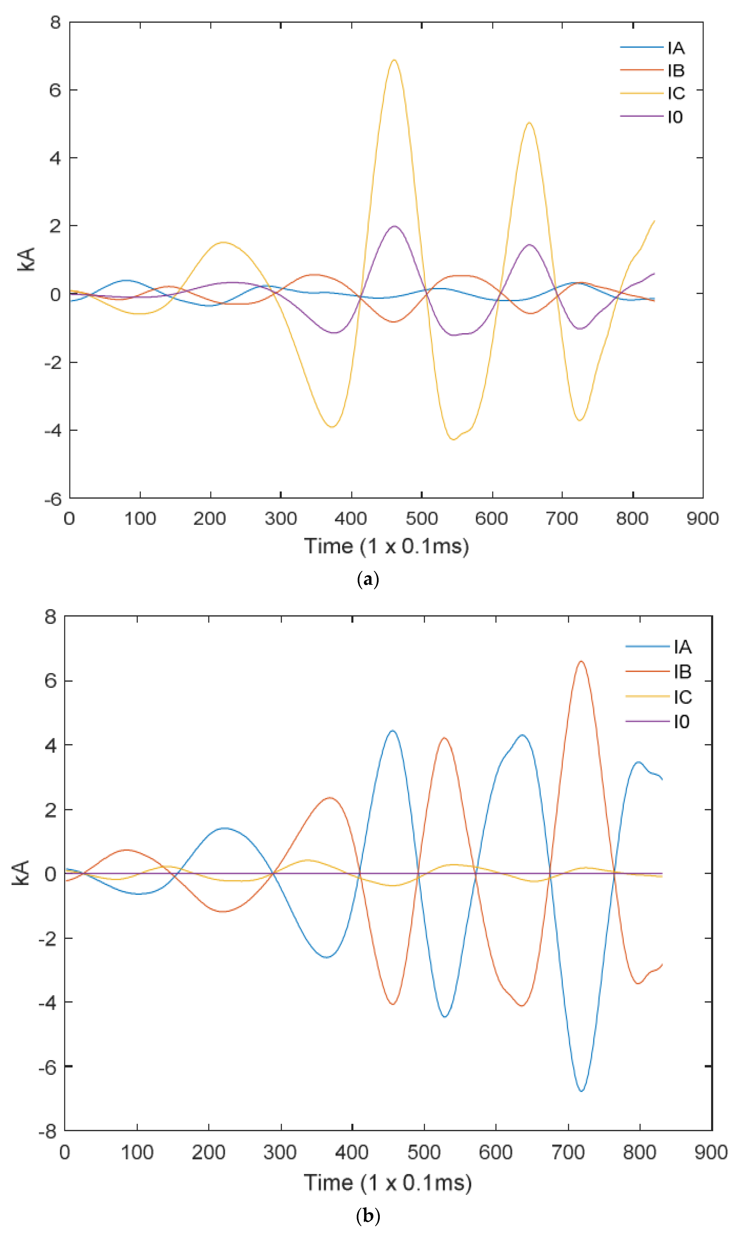
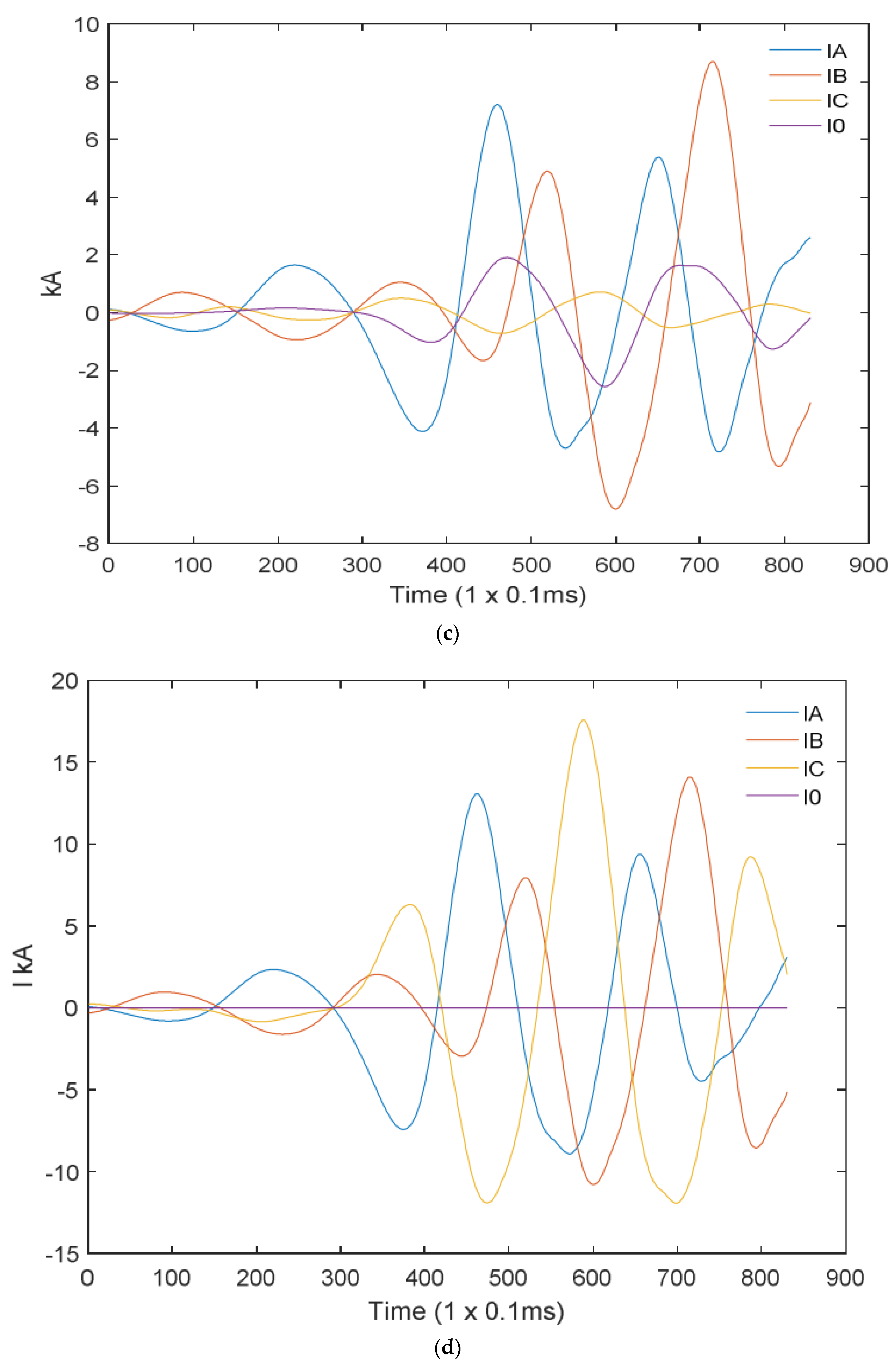
Fault occurrences take place when there is an insulation failure between the phase conductor and the ground and between the phase conductors. When the insulation fails, the current magnitude at the point of the fault increases beyond the nominal current limit rapidly. The fault types are classified as (a) single line-to-ground (SLG), (b) line-to-line (LL), (c) double line-to-ground (LLG), and (d) triple line fault (LLL) [2]. In modern power distribution protection systems, intelligent electronic devices (IEDs) are utilized to monitor any disturbances that may occur in the system. IEDs mostly use discrete Fourier transforms (DFT) for signal interpretation. However, the main drawback of DFTs for power system applications is the time resolution due to a high-frequency resolution being required [3].

In recent past years, many researchers have investigated fault classification and estimation schemes for power distribution systems. The design of these schemes follows the architecture of (i) signal measurement, (ii) signal decomposition and analysis, (iii), feature extraction and selection, (iv) fault classification, and (v) fault location. A hybrid protection scheme based on wavelet transform (WT) and probabilistic neural network (PNN) was proposed for fault classification in a power system [4]. The scheme utilized the WT technique for signal processing and feature extraction. The extracted features from WT are fed into the PNN algorithm for fault classification. The studies in [5,6] proposed protection schemes based on the combination of WT and fuzzy logic (FL). In these studies, WT was employed for signal decomposition, and FL was used for fault classification. In these schemes, a simple computation process is used; however, the classification error reported is largely due to inconsistent simulation conditions. In [7], a technique based on WT for fault detection in a transmission line was proposed. The techniques used Daubechies 4 (db4) mother wavelet for signal tracking and analysis. In [8], a technique based on discrete wavelet transform (DWT), an artificial neural network (ANN), and an extreme learning machine (ELM) for distribution fault detection were proposed. The proposed technique used DWT for signal processing and feature extraction, the ANN algorithm was used to classify different types of faults, and ELM was used for fault location. The scheme produced good results with minimal time delay. Guo et al. proposed a deep learning fault detection technique based on the Hilbert–Huang transform (HHT) and a convolutional neural network (CNN) [9]. The technique uses HHT to extract energy features from the fault signal, and CNN is employed for fault classification. An adaptive protection scheme based on ANN and WT for fault detection was proposed in [10]. The scheme produced good results; however, fault location was not considered. In [11], a technique based on stationary wavelet transform (SWT) and support vector machine (SVM) was proposed. The technique used SWT for signal decomposition and feature extraction, while the SVM scheme was used for fault classification and detection.

Fault location is another important aspect to consider when designing a protection scheme. Fault location schemes give an indication of where the fault has occurred along the power distribution line, resulting in a much quicker restoration time. In [12], a technique based on ANN and a deterministic approach (DA) to locate the fault in a distribution line is proposed. However, it is reported in [12] that the estimation fault error is high. Fault location schemes were proposed in [13,14]. These schemes use the ANN technique to estimate the fault position and WT to extract statistical features to train and test the ANN location scheme. In [15], the authors used DWT and wavelet fuzzy neural network (WFNN) to estimate the fault position. DWT is used to extract statistical features from the fault signal, and WFNN is used to determine the fault location. An intelligent fault location scheme based on wavelet packet transform (WPT) and back propagation neural network (BPNN) techniques was proposed [16]. The scheme in [16] used WPT as a feature extraction algorithm and BPNN as a fault estimator. A fault location scheme based on determinant function and support vector regression (SVR) is discussed in [17]. The scheme in [17] considered the measurements of both current and voltage at the terminal source. Furthermore, a filtering segment of the noise and DC offset is used in [17] to improve the scheme’s efficiency. In [18], a hybrid protection scheme for fault location in a distribution radial network using WT and SVR is proposed. The scheme in [18] uses DWT for feature extraction and SVR to estimate the location of the fault. Although several schemes have been proposed to determine an optimal solution to the fault diagnostic problem. The limitations of these schemes cannot be ignored. The limitations range from signal analysis, parameter selection, and the time taken to respond to the fault. In our study, we propose a more reliable signal analysis tool. We further use optimization techniques to determine the parameters of the classifier to enhance the classification accuracy. Unlike other proposed schemes, our scheme uses half of a cycle of the post-fault signal to classify and estimate the fault position, thus improving the processing time.

This paper proposes two hybrid methodologies for fault classification and locating in a distribution power line. The proposed method focuses on the analysis of a single cycle of the current signal, which is extracted from the sending end terminals of the distribution power line under consideration for fault classification and locating. Subsequently, the current samples are processed using the wavelet packet transform, and statistical features are extracted from them. Unlike other schemes discussed that use one or more cycles, our scheme uses half a cycle of the post-fault signal. The training data are generated through simulation, and conditions such as fault impedances, fault incipient angles, and fault distances are considered. The statistically selected features are then used to train and test the SVM classifier and SVR locator. The optimal performance of the SVM and SVR schemes is improved by using the particle swarm optimization technique to determine the optimal parameters. To minimize the complexity of the scheme, four support vector classifiers (SVC) are used to detect the fault in the corresponding phases and the ground. The sampling period is taken to be 12.5 kHz for the whole process. The simulation results depict that the proposed scheme can classify and locate power systems faults with high accuracy and minimal estimation error. The remainder of the paper is organized as follows: In Section 2, the wavelet and feature extraction techniques are discussed. Section 3 discusses the support vector machines for fault classification and locating. In Section 4, the proposed SVC and SVR fault classification and regression techniques are discussed. Section 5 discusses the power system case study. In Section 6, the results are discussed. Section 7 reports the fault classification and location in a grid-integrated system with renewable energy sources, and in Section 8, a conclusion is drawn.

2. Wavelet Transforms and Feature Extraction

Signal processing and tracking form an integral part of the whole protection value chain. The DWT and WPD have emerged as powerful signal-processing tools. These tools have been used numerously in power systems to analyze signals of interest [19]. The DWT and WPD are orthogonal wavelets where a signal is passed through numerous filters. Considering the signal $\left(S\right)$, if DWT is employed, the signal is passed through the low- and high-pass filters simultaneously. The output of the high-pass filter (HPF) and low-pass filter (LPF) correspond to the detail and approximation coefficients, respectively, as depicted in Figure 1. The figure indicates that the detail coefficient information is lost at every level of decomposition. For instance, if there are $l$ levels of decompositions, there would be $\left(l+1\right)$ possible ways to decompose the signal.

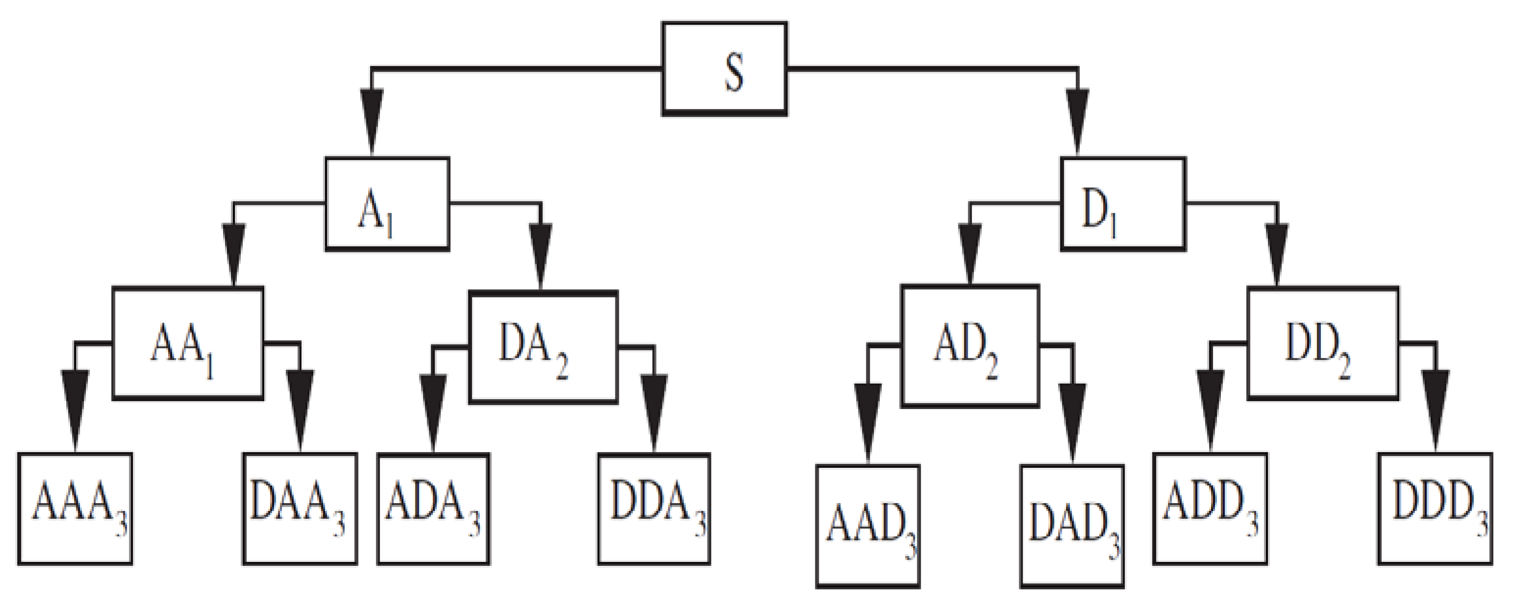
However, unlike DWT, in the case of WPD, the signal is passed through multiple filters on both approximation and detail coefficients. Considering the signal $\left(S\right)$, if WPD is employed, the signal is passed through the low- and high-pass filters simultaneously, as depicted in Figure 2. Thereafter, the approximation and detail coefficients are further decomposed to level $k$. The approximation and detail coefficients are further decomposed simultaneously at every level, resulting in more information, and a high-frequency resolution compared to the DWT technique [20]. The low-pass filter $f\left(x\right)$ and the high-pass filter $h\left(x\right)$ are mathematically expressed as:

$$W_{2n}\left(x\right)=\sqrt{2}{\displaystyle \sum }_{k=0}^{2N-1}f\left(x\right)W_n\left(2x-k\right)$$

(1)

$$W_{2n+1}\left(x\right)=\sqrt{2}{\displaystyle \sum }_{k=0}^{2N-1}g\left(x\right)W_n\left(2x-k\right)$$

(2)

where $n$ is the number of decomposition coefficients, $W_0=\mathsf{\Phi }\left(x\right)$ is the scaling factor, and the wavelet function is given by $W_1=\mathsf{\psi }\left(x\right)$. Feature extraction is a mathematical technique used to transform a large data spectrum into a small data spectrum without losing critical information. In power system applications, feature extraction is mostly used to improve computation processing time. In the present work, we extract statistical features from the fault signal to improve the protection scheme efficiency. The features are extracted at each level of decomposition, and a feature matrix is then developed. The statistical features extracted from the fault signal are defined mathematically as:

2.1. Standard Deviation and Mean Value

The standard deviation $\left(\sigma \right)$ of the signal is a measure of how the signal deviates from its own mean value and is mathematically expressed as:

$$\sigma \left(t_1,t_2\right)=\sqrt{\left({{\displaystyle \int }}_{t_1}^{t_2}\left(x\left(t\right)-\overline{x}\right)dt\right)}$$

(3)

where $\left(t_1,t_2\right)$ denotes the time limit of signal $x\left(t\right)$, and $\overline{x}$ is the mean average and is mathematically expressed as:

$$\overline{x}=\frac{1}{t_2-t_1}{{\displaystyle \int }}_{t_1}^{t_2}x\left(t\right) dt$$

(4)

Under no-fault conditions, $\mathsf{\sigma }=1$, and under fault conditions the value deviates from one. The mean ($\overline{\mathrm{x}})$ value of the signal is the average value of the signal and is equal to zero under normal conditions; the ($\overline{\mathrm{x}})$ value is not equal to zero under fault conditions.

2.2. Energy

The energy $\left(E\right)$ of signal $x\left(t\right)$ is mathematically expressed as:

$$E\left(t_1,t_2\right)={{\displaystyle \int }}_{t_1}^{t_2}{\left(\left|x\left(t\right)\right|\right)}^2 dt$$

(5)

The energy of the signal under fault conditions is greater than the energy of the signal under normal power system conditions.

2.3. Kurtosis

The kurtosis $\left(K\right)$ of a signal is the measure of the signal’s uniformity. The kurtosis $\left(K\right)$ of the signal is expressed mathematically as:

$$K\left(t_1,t_2\right)={{\displaystyle \int }}_{t_1}^{t_2}{\left(\frac{x\left(t\right)-\overline{x}}{\sigma }\right)}^4$$

(6)

Under normal conditions, $K=3$, and $K>3$ under fault conditions.

2.4. Skewness

The skewness $\left(S\right)$ of a signal is the measure of the signal’s asymmetry relative to the mean average of the signal. The skeweness $\left(S\right)$ of a signal is mathematically defined as:

$$S\left(t_1,t_2\right)=\frac{{{\displaystyle \int }}_{t_1}^{t_2}{\left(x\left(t\right)-\overline{x}\right)}^3}{{\sigma }^3}$$

(7)

Under normal conditions $S=0$, and under fault conditions $S\ne 0$. Ultimately, these features are formulated in a matrix and the feature matrix $F_S$ is given by:

$$F_S=\left[\begin{array}{ccc}\begin{array}{c}\sigma \\ ⋮\\ \begin{array}{c}⋮\\ \begin{array}{c}⋮\\ \begin{array}{c}⋮\\ {\sigma }_n\end{array}\end{array}\end{array}\end{array}& \begin{array}{c} \overline{x}\\ ⋮\\ \begin{array}{c}⋮\\ \begin{array}{c}⋮\\ \begin{array}{c}⋮\\ {\overline{x}}_n\end{array}\end{array}\end{array}\end{array}& \begin{array}{ccc}\begin{array}{c} E\\ ⋮\\ \begin{array}{c}⋮\\ \begin{array}{c}⋮\\ \begin{array}{c}⋮\\ E_n\end{array}\end{array}\end{array}\end{array}& \begin{array}{c}K\\ ⋮\\ \begin{array}{c}⋮\\ \begin{array}{c}⋮\\ \begin{array}{c}⋮\\ K_n\end{array}\end{array}\end{array}\end{array}& \begin{array}{c}S\\ ⋮\\ \begin{array}{c}⋮\\ \begin{array}{c}⋮\\ \begin{array}{c}⋮\\ S_n\end{array}\end{array}\end{array}\end{array}\end{array}\end{array}\right]$$

(8)

3. Support Vector Machines for Fault Classification and Location

In statistical theory, support vector machines (SVMs) were initially established as (SVC) to solve classification and pattern recognition problems. When employing SVMs, the input datasets are mapped into a high dimensional space to establish the hyperplane. The hyperplane is defined as a separating margin line between two different classes of data [21]. The hyperplane is determined by solving the quadratic programming optimization problem given by:

$$min\frac{1}{2}{\left|w\right|}^2+C\left({\displaystyle \sum }_{i=1}^l{\zeta }_i\right)$$

(9)

subject to

$$y_1\left(w·x_i+b\right)\ge 1-{\zeta }_i,{\zeta }_i\ge \forall i$$

where $x_i$ denotes the $ith$ term of the class data, $C$ is the pre-determined constant, ${\zeta }_i$ is the loss function, and $y_i$ is the classification output, which is given by $\left[+1,-1\right]$. The optimization problem in (9) can be solved by using the dual form expressed as:

$$max{L}_D={\displaystyle \sum }_i{\alpha }_i-\frac{1}{2}{\displaystyle \sum }_{i,j}{\alpha }_i{\alpha }_j{y}_i{y}_j\left(x_i^T{x}_j\right)$$

(10)

subject to $0\le {\alpha }_i\le C\forall i,{\displaystyle \sum }_i{y}_i$.

In most practical cases, the data are not displaced linearly and thus cannot be separated using a linear hyperplane. For such cases, kernel functions are used to determine an optimal hyperplane. The commonly used kernel functions are quadratic, polynomial, radial bias function (RBF), and sigmoid [22]. The application of SVMs can be extended to solve regression problems. In the present work, we used four (4) SVCs to classify different faults on different phases and on the ground. The classification training matrix of the SVCs is depicted in

Table 1. SVC training matrix accuracy.

Fault Type	SVCA	SVCB	SVCC	SVCG	Accuracy (%)
LAG	+1	−1	−1	+1	100
LBG	−1	+1	−1	+1	100
LCG	−1	−1	+1	+1	100
LALB	+1	+1	−1	−1	100
LALC	+1	−1	+1	−1	100
LBLC	−1	+1	+1	−1	100
LALBG	+1	+1	−1	+1	100
LALCG	+1	−1	+1	+1	100
LBLCG	−1	+1	+1	+1	100
LALBLC	+1	+1	+1	−1	100

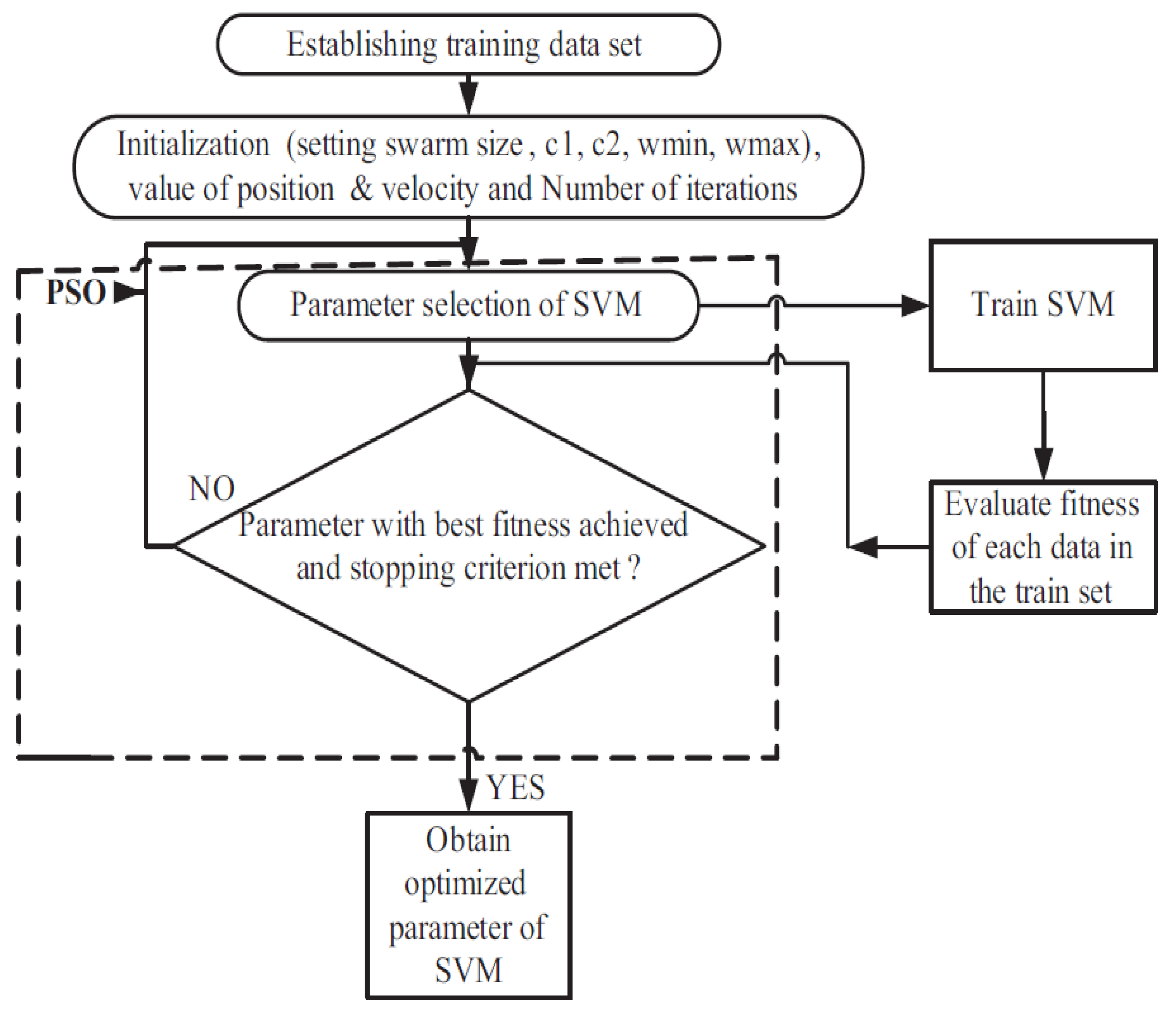
. In Table 1, SVC_A, SVC_B, SVC_C, and SVC_G correspond to classifying the fault in phases A, B, C, and the ground, respectively. Furthermore, the parameters of the SVC classifiers are optimized by using the particle swarm optimization (PSO) technique. The fitness $f$ of the PSO technique is determined by calculating the mean square error (MSE) value, expressed as:

$$f=\sqrt{\frac{1}{N}{\displaystyle \sum }_{k=1}^N{\left[y^{\mathsf{\Lambda }}\left(k\right)-y\left(k\right)\right]}^2}$$

(11)

where $y\left(k\right)$ denotes the discrete signal, $y^{\mathsf{\Lambda }}\left(k\right)$ is the forecasted SVC output, and the number of data samples is denoted by $N$. The optimal SVC values are selected using the PSO technique during the training procedure. The architecture design for selecting optimal SVM parameters for classification is depicted in Figure 3. The process begins with establishing the training data using the fault current magnitude. Thereafter, the data are processed to determine the PSO parameters. Subsequently, the data are used to train the SVM for classification and regression. The evaluation of fitness is determined by using the (MSE) technique. Lastly, a decision is determined, if the best parameters are not determined, the data are reprocessed, otherwise the parameters are used to implement the SVM technique.

In the present work, we use support vector regression (SVR) to estimate the fault position along the distribution power line. The SVR problem can be solved by determining the quadratic optimization problem and introducing a set of dual variables ${\alpha }_i,{\alpha }_i^{*}$ and thereafter constructing the Lagrange function. The optimal mapping into the high-dimensional space is achieved by computing the dot product using the kernel function. Therefore, the mathematical formulation is expressed as in (11):

$$max W\left(\alpha ,{\alpha }^{*}\right)=\frac{1}{2}{\displaystyle \sum }_{i,j=1}^l\left({\alpha }_i-{\alpha }_i^{*}\right)\left({\alpha }_j-{\alpha }_j^{*}\right)K\left(X_i,X_j\right)+{\displaystyle \sum }_{i,j=1}^l\left({\alpha }_i^{*}-{\alpha }_i\right)y_i-\frac{1}{2C}{\displaystyle \sum }_{i=1}^l{\alpha }_i^2-{\alpha }_i^{*2}$$

(12)

where $K\left(X_i,X_j\right)$ denotes the kernel function. In the present work, we choose the RBF function.

4. Proposed Fault Classification and Location

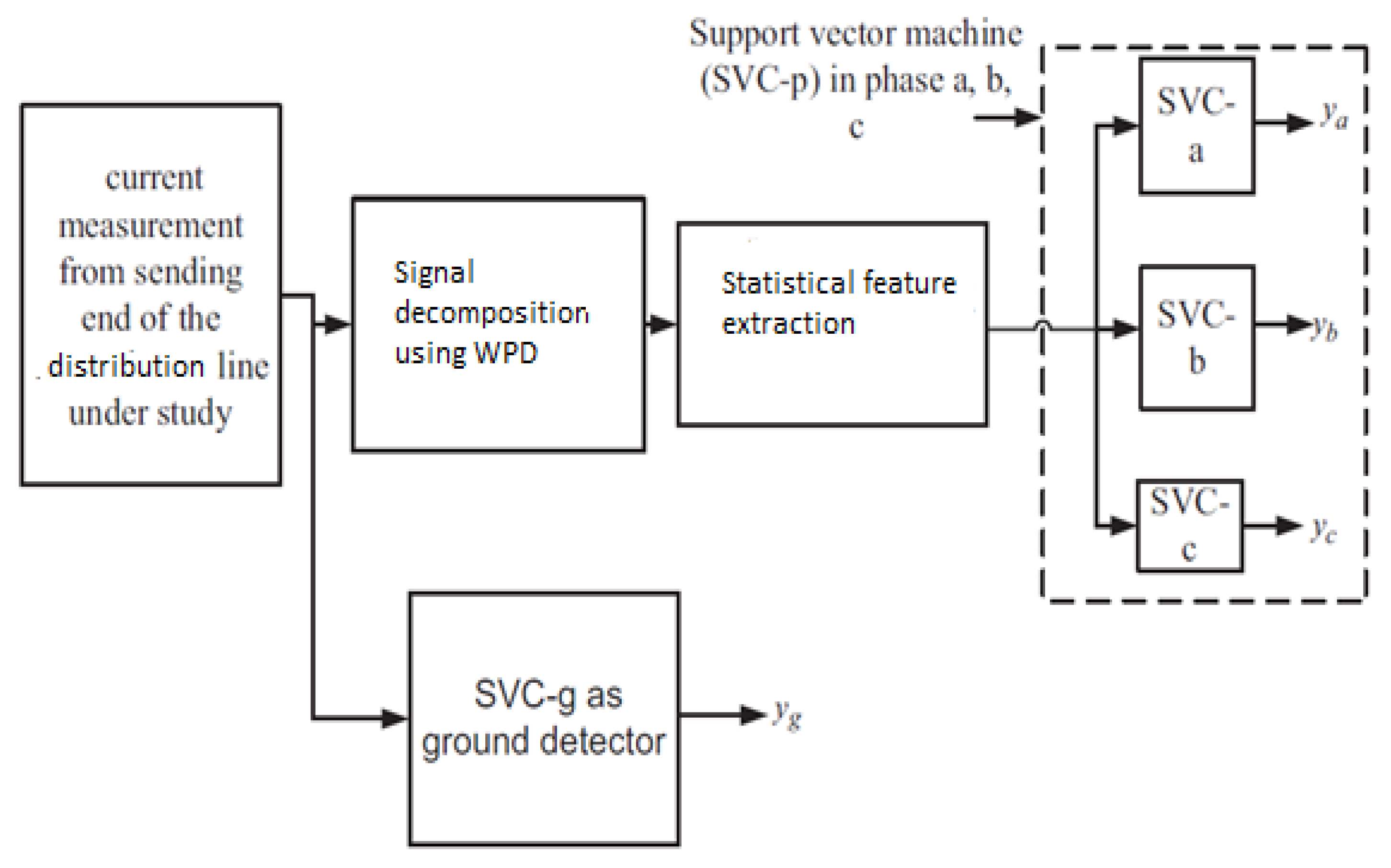
In this section, the proposed fault classification and detection scheme is discussed. The fault classification scheme is depicted in Figure 4.

The process of fault classification begins with the post-fault measurement at the source terminal. Thereafter, the measured current is passed through numerous filters using the WPD tool. Subsequently, statistical features are extracted from the decomposed signal at level 4. The total features are 80 (16 WPD coefficients $\times$5 statistical features). The statistical features are used to formulate a future matrix. The feature matrix is used to train the SVM for classification. The SVM optimal parameters are obtained using the PSO. To reduce the computational complexity, four (4) SVCs are used to classify the faults corresponding to each phase and the ground. In most cases, the line-to-line (LL) fault is misclassified as the line-to-line-to-ground (LLG) fault. In the present work, the misclassification problem is solved by installing the ground SVC at the generating source, as depicted in Figure 5.

The fault location scheme begins with the fault current measurements at the terminal source. The measured current is passed through several filters and decomposed to level 4 using WPD. Thereafter, the extracted features are used to test and train the SVR locator to estimate the position of the fault. The performance of the fault estimation scheme is determined by calculating the mean square error (MSE) and the absolute error (AE). The absolute error is expressed mathematically as:

$$AE=\left|A_{FD}-E_{FP}\right|$$

(13)

where $A_{FP}$ is the actual fault position, and $E_{FP}$ is the estimated fault position. A high $AE$ means that the scheme is out of range and produces inaccurate results.

5. Power System Simulation under Study

To validate our scheme, we used an Eskom power distribution line as a case study. Eskom is a South African power utility responsible for supplying more than 95% of electricity for industrial and household applications. A reduced power system segment of the Eskom distribution line is shown in Figure 6. The network is modeled as a two-substation system. The voltage at the sending end and receiving end of the line is rated at 132 kV voltage supply. The distribution network is modeled as a pi-type system with a total length of 155 km. The modeling of the network is subdivided into small sections to improve model design and efficiency. The substation parameters are depicted in

Table 2. Substation parameters.

Source	Apparent Power (MVA)	Fault Level (kA)
Substation A	20	55.5
Substation B	15	42.3

.

The parameter value of the resistor $R \left(\mathsf{\Omega }\right)$, inductor $L \left(\mathrm{H}\right)$, and capacitor $C\left(\mathrm{F}\right)$ of the distribution line per kilometer are given in Equations (14)–(16), respectively.

$$R=\left[\begin{array}{ccc}0.15& 0.12& 0.12\\ 0.12& 0.15& 0.12\\ 0.12& 0.12& 0.15\end{array}\right] \Omega /\mathrm{k}\mathrm{m}$$

(14)

$$L=\left[\begin{array}{ccc}1.12e^{-3}& 1.90e^{-3}& 6.30e^{-3}\\ 1.90e^{-3}& 1.12e^{-3}& 1.90e^{-3}\\ 6.30e^{-3}& 1.90e^{-3}& 1.12e^{-3}\end{array}\right] H/\mathrm{k}\mathrm{m}$$

(15)

$$C=\left[\begin{array}{ccc}1.10e^{-8}& -2.85e^{-9}& -6.40e^{-10}\\ -2.85e^{-9}& 1.10e^{-8}& -2.85e^{-9}\\ -6.40e^{-10}& -2.85e^{-9}& 1.10e^{-8}\end{array}\right] F/\mathrm{k}\mathrm{m}$$

(16)

The power distribution system used in the present work for analysis is modeled in the MATLAB/Simulink platform. The power system could have been modeled in any other power system platform, such as (DigSilent, PLSCAD, and ATPDraw) without any significant difference in the results. Eleven (11) types of faults are initiated at different locations of the distribution line to develop a fault data matrix. The proposed fault classification and location schemes use half a cycle of the post-fault signal. The (LG), (LL), (LLG), and (LLL) fault signals are shown in Figure 7. It is observed from Figure 7 that the current magnitude increases drastically when a fault occurs.

6. Results and Discussion

In this section, we discuss the results of our proposed fault classification and location schemes. In the present work, WPD is used to analyze and decompose the fault current signal to improve the scheme’s efficiency. The accuracy and performance of the WPD depend on the type of the mother wavelet. In [23], it was reported that the Daubechies (db.) mother wavelet performs better for transient signal analysis. In

Table 3. Mother wavelet selection criterion.

Mother Wavelet	Fault Classification	Fault Location
	Fault Classification Accuracy (%)	Mean Error (%)	Mean Square Error (%)
db1	96.7	0.51	1.02
db2	94.8	0.33	0.52
db3	91.3	0.41	0.35
db4	99.5	0.10	0.21

, different mother wavelets are tested to measure the classification and location schemes. It is observed in

Table 4. Training and testing data.

Data Matrix Sets	Fault Impedance (Ω)	$\mathbf{Fault}\mathbf{Angle}(\mathsf{\Phi })$
Training data	1.5, 10, 15, 75, 100, 150, 220, 260	10° 15°, 20°, 40°, 85°
Test data	1.0 30, 45, 110, 165, 180, 210, 300	30°, 80°, 110°, 140°, 190°

that db4 shows high classification accuracy (99.5%) and a mean error of (0.10%), which is better compared to the other mother wavelets. The training and testing datasets used in the study are shown in Table 4. In

Table 5. Feature selection of SVM using PSO.

SVM	Fault Classification	Fault Location
Kernel function	Radial bias function	Radial bias function
Gamma $\left(\gamma \right)$	0.42	0.42
Cost $(c)$	11.30	13.80
Nu $\left(nu\right)$	0.55	0.55

, the SVM parameters obtained using the PSO are shown. In this paper, the indices used to determine the classification performance are the true positive (TP), false positive (FP), precision, recall, and the receiver operating characteristics (ROC). The TP and FP indicate the probability of the positive and negative rate outputs, the precision indicates the fraction of pertinent instances among recovered instances, the recall is the fraction of instances that were recovered, and the ROC illustrates the diagnostic ability of the classifier when the threshold is varied.

The SVM performance results using different sample cycle delays are presented in

Table 6. SVM classification with half a cycle post-fault.

Fault Type	TP	FP	Precision	Recall	F-Measure	ROC
AG	0.991	0.000	1.000	1.000	0.991	0.970
BG	0.920	0.000	0.991	0.990	0.990	0.966
CG	0.933	0.000	0.990	0.980	0.995	0.985
AB	0.985	0.000	0.998	0.985	0.977	0.990
AC	0.968	0.003	0.990	0.930	0.988	0.900
BC	0.987	0.000	1.000	0.975	0.970	0.988
ABG	0.980	0.014	0.990	0.957	0.966	0.955
ACG	0.981	0.010	1.000	0.911	0.960	0.975
BCG	0.971	0.035	0.999	0.980	0.991	0.961
ABC	0.981	0.043	0.990	0.990	0.955	0.992
Avg	0.969	0.011	0.995	0.970	0.978	0.968

,

Table 7. SVM classification with single cycle post-fault.

Fault Type	TP	FP	Precision	Recall	F-Measure	ROC
AG	0.902	0.000	0.915	0.990	0.905	0.955
BG	0.915	0.000	0.943	0.955	0.922	0.950
CG	0.945	0.000	0.955	0.965	0.959	0.980
AB	0.955	0.000	0.940	0.952	0.960	0.970
AC	0.915	0.003	0.933	0.911	0.977	0.911
BC	0.920	0.010	0.990	0.933	0.950	0.916
ABG	0.991	0.000	0.982	0.960	0.960	0.958
ACG	0.900	0.010	0.922	0.915	0.955	0.988
BCG	0.980	0.050	0.985	0.930	0.965	0.966
ABC	0.975	0.045	0.975	0.945	0.977	0.911
Avg	0.941	0.012	0.954	0.946	0.953	0.951

and

Table 8. SVM classification with two cycles post-fault.

Class	TP	FP	Precision	Recall	F-Measure	ROC
AG	0.991	0.000	0.960	1.000	0.991	0.970
BG	0.920	0.000	0.991	0.990	0.990	0.966
CG	0.933	0.000	0.990	0.980	0.995	0.985
AB	0.985	0.000	0.961	0.985	0.977	0.990
AC	0.968	0.003	0.950	0.930	0.988	0.900
BC	0.987	0.000	0.910	0.975	0.970	0.988
ABG	0.980	0.014	0.960	0.957	0.966	0.955
ACG	0.981	0.010	0.988	0.911	0.960	0.975
BCG	0.971	0.035	0.991	0.980	0.991	0.961
ABC	0.981	0.043	0.950	0.990	0.955	0.992
Avg	0.969	0.011	0.965	0.970	0.978	0.968

. Table 6, Table 7 and Table 8 show that the average precision classification accuracy is 99.5% when half a sample cycle is used compared to 95.4% and 96.5% when using one and two cycles post-fault. Thus, in our scheme, the half-cycle samples are used. Furthermore, the classification accuracy of the SVM in each phase is shown in

Table 9. Fault classification accuracy on different phases.

Fault Type	No. of Instances	No. of Instances Correctly Classified	No. of Instances Incorrectly Classified	Accuracy (%)
LG	25,400	25,400	0.000	100
LL	25,400	25,250	150.0	99.4
LLG	25,400	25,085	315.0	98.8
LLL	25,400	25,357	43.00	99.8
Total	101,600	101,092	508.0	99.5

. The classification accuracy is determined by calculating the ratio between the correctly classified instances and the total instances tested.

Moreover, the number of samples is used to test the SVR scheme for the fault location. The results of the fault estimation distance using different fault impedance, fault angle incipient, and fault locations are depicted in

Table 10. Fault estimation at 45 and 90 km with a 10 Ω fault impedance.

Fault Type		45 km			90 km
	0°	30°	60°	0°	30°	60°
LG	45.0	44.9	45.0	89.9	90.0	90.0
LL	45.0	45.0	45.0	90.0	90.0	90.0
LLG	44.9	45.0	44.9	90.0	90.0	90.0
LLL	45.0	45.0	43.9	90.0	90.0	90.0

and

Table 11. Fault estimation at 110 and 90 km with a 20 Ω fault impedance.

Fault Type		110 km			140 km
	0°	30°	60°	0°	30°	60°
LG	110.0	110.0	110.0	139.9	135.0	140.0
LL	109.8	109.0	110.0	140.0	138.0	139.0
LLG	109.5	110.0	109.9	140.0	140.0	140.0
LLL	110.0	110.0	110.0	140.0	140.0	140.0

. The results in Table 10 and Table 11 show that the SVR scheme is able to estimate the fault location with a minimum error irrespective of the fault angle and impedance. Moreover,

Table 12. AE at 45 and 90 km with a 10 Ω fault impedance.

Fault Type		45 km			90 km
	0°	30°	60°	0°	30°	60°
LG	0.00	0.01	00.0	0.10	0.00	0.00
LL	0.00	0.00	0.00	0.00	0.00	0.00
LLG	1.00	0.00	00.1	0.00	0.00	0.00
LLL	0.00	0.00	0.00	00.0	0.00	0.00

and

Table 13. AE at 110 and 140 km with a 20 Ω fault impedance.

Fault Type		110 km			140 km
	0°	30°	60°	0°	30°	60°
LG	0.00	0.00	0.00	0.10	5.00	0.00
LL	0.20	1.00	0.00	0.00	2.00	1.00
LLG	0.50	0.00	0.90	0.00	0.00	0.00
LLL	0.00	0.00	0.00	0.00	0.00	0.00

depict the summary of the absolute error between the actual fault position and the estimated fault position. Most of the fault instances are accurately located with a minimum margin of error.

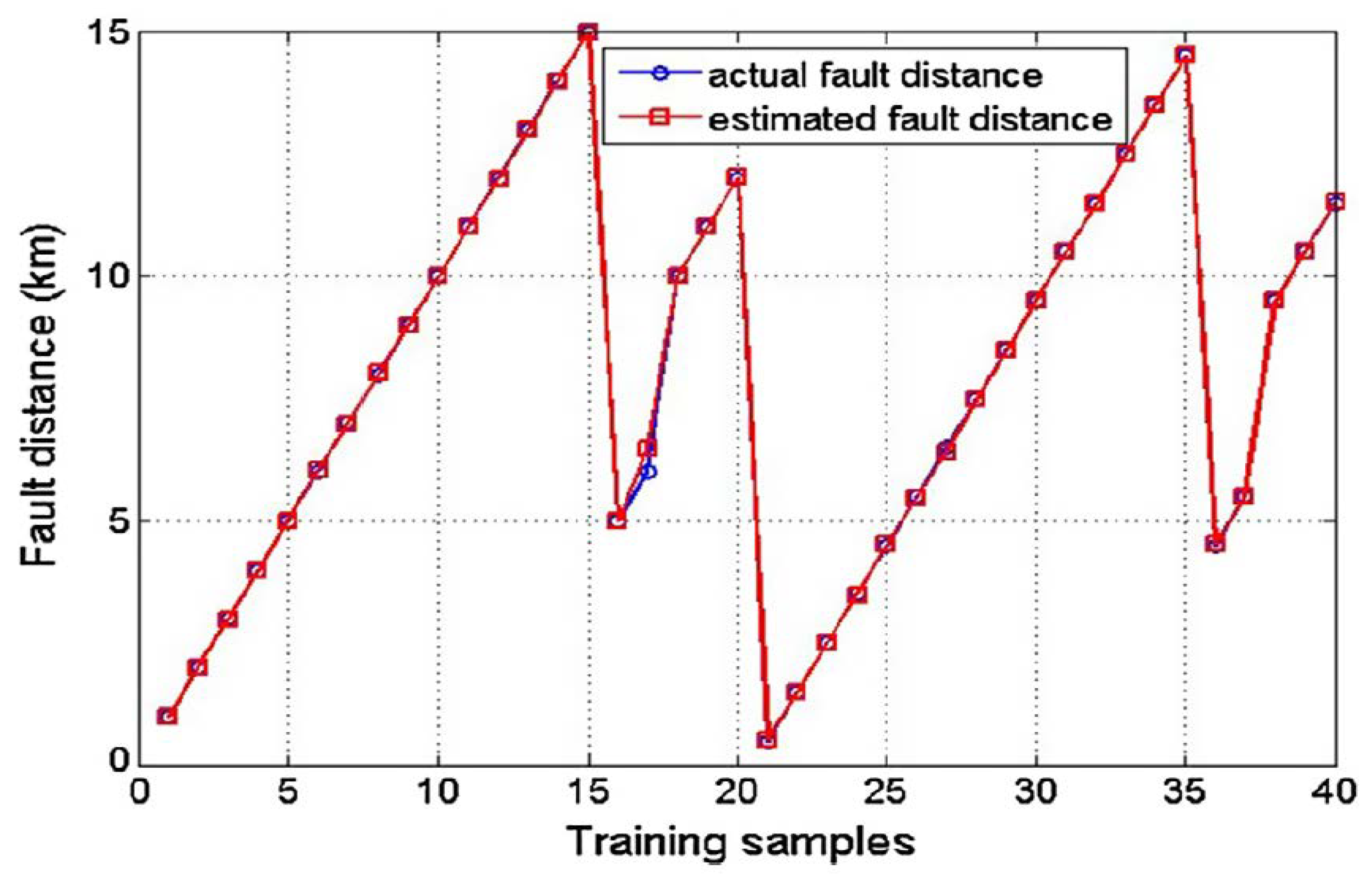
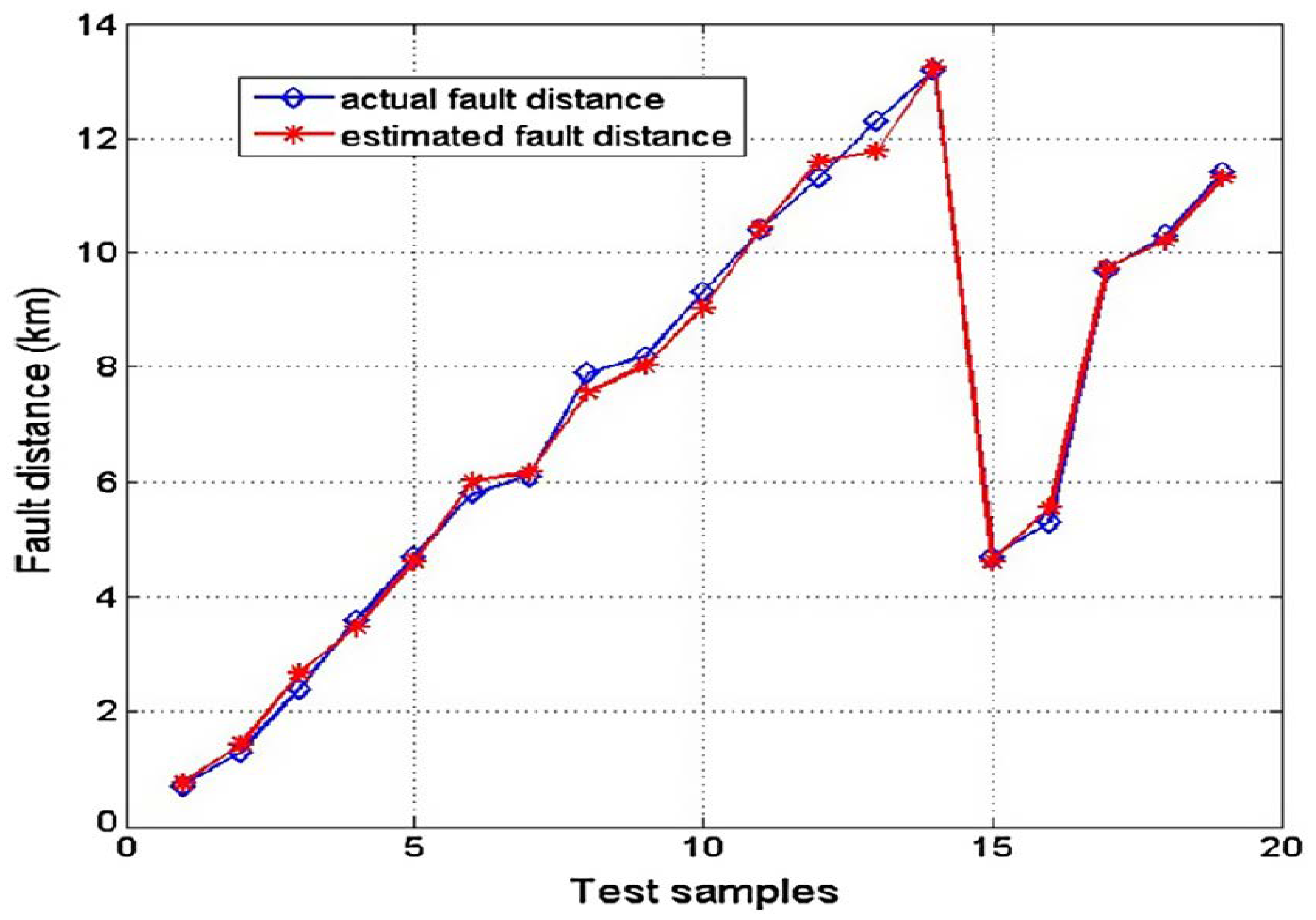
The estimation results of the training data samples for a single phase to ground fault are depicted in Figure 8. From Figure 8, it can be seen that the SVR scheme has a good training outcome. To verify the unknown fault distance, the single phase to the ground instance is used, and the results are depicted in Figure 9. It can be noted from Figure 9 that the scheme is able to estimate the fault position with a minimum error of 0.0010.

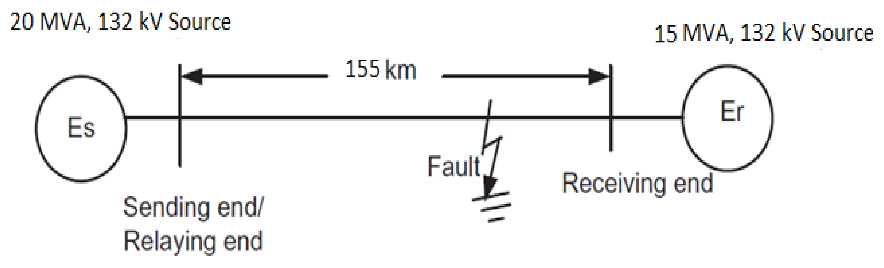
7. Fault Classification and Location with Renewable Energy Distributed Generation Integration

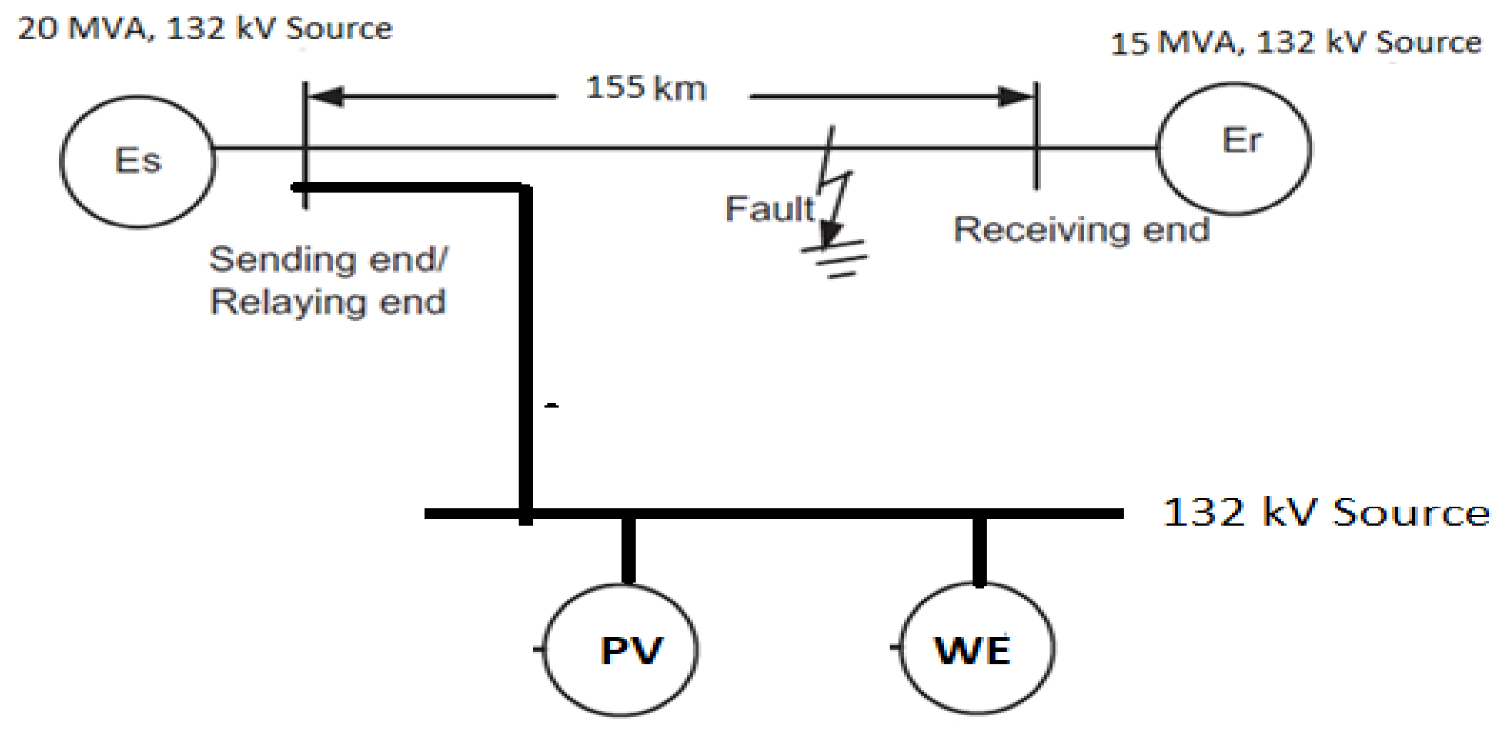
The electricity trajectory has evolved over the years with the more decentralized energy generation sources. In most cases, renewable energy sources (RES) have been used to enhance the electricity supply and security. However, there are technical dynamics that are introduced by these technologies. In the present work, we investigate the validity of the proposed fault classification and detection on a hybrid integrated system with RES. The wind energy (WE) and photovoltaic (PV) source parameters are given in

Table 14. RES parameters.

Parameter	WE Source	PV Source
Voltage (kV)	132	132
Fault level (kA)	1.34	0.91
Power factor	0.9 lag	1.00
Power (kW)	15.50	6.33

. The integrated network used to validate our proposed scheme is depicted in Figure 10.

The performance of SVM using the half, single, and two post-fault cycles is presented in

Table 15. SVM classification from half a cycle post-fault with PV and WE sources.

Fault Type	TP	FP	Precision	Recall	F-Measure	ROC
AG	0.988	0.000	0.990	0.905	0.982	0.910
BG	0.900	0.000	0.981	0.955	0.922	0.955
CG	0.921	0.030	0.970	0.951	0.991	0.958
AB	0.980	0.045	0.968	0.958	0.955	0.909
AC	0.952	0.033	0.970	0.903	0.951	0.922
BC	0.911	0.022	1.000	0.957	0.966	0.975
ABG	0.899	0.055	0.960	0.975	0.952	0.966
ACG	0.855	0.099	1.000	0.971	0.922	0.952
BCG	0.950	0.011	0.955	0.908	0.981	0.916
ABC	0.991	0.044	0.980	0.909	0.931	0.929
Avg	0.935	0.034	0.977	0.939	0.955	0.939

,

Table 16. SVM classification with a single cycle post-fault with PV and WE sources.

Fault Type	TP	FP	Precision	Recall	F-Measure	ROC
AG	0.900	0.000	0.910	0.900	0.922	0.950
BG	0.910	0.000	0.912	0.965	0.955	0.944
CG	0.911	0.000	0.922	0.950	0.960	0.923
AB	0.920	0.000	0.904	0.900	0.925	0.962
AC	0.900	0.000	0.905	0.920	0.930	0.901
BC	0.902	0.000	0.909	0.925	0.922	0.921
ABG	0.919	0.000	0.920	0.977	0.920	0.922
ACG	0.910	0.030	0.930	0.922	0.922	0.908
BCG	0.908	0.080	0.955	0.940	0.925	0.922
ABC	0.957	0.010	0.966	0.930	0.940	0.933
Avg	0.914	0.012	0.923	0.933	0.923	0.929

and

Table 17. SVM classification with two cycles post-fault with PV and WE sources.

Class	TP	FP	Precision	Recall	F-Measure	ROC
AG	0.919	0.000	0.906	0.902	0.981	0.930
BG	0.902	0.000	0.919	0.920	0.960	0.926
CG	0.911	0.000	0.909	0.908	0.955	0.955
AB	0.958	0.000	0.916	0.922	0.927	0.940
AC	0.911	0.003	0.905	0.903	0.948	0.910
BC	0.925	0.000	0.900	0.943	0.920	0.928
ABG	0.908	0.012	0.906	0.951	0.916	0.955
ACG	0.922	0.000	0.944	0.922	0.920	0.945
BCG	0.917	0.025	0.920	0.908	0.911	0.931
ABC	0.925	0.012	0.925	0.909	0.945	0.952
Avg	0.920	0.008	0.915	0.919	0.938	0.937

. The results presented in Table 15, Table 16 and Table 17 show that the precision accuracy of the SVM scheme using half a cycle’s data post-fault is 97.7%, compared to 92.3% and 91.5% when using a single and two cycles of the post-fault data. In

Table 18. Fault classification accuracy in different phases with PV and WE sources.

Fault Type	No. of Instances	No. of Instances Correctly Classified	No. of Instances Incorrectly Classified	Accuracy (%)
LG	25,400	25,400	0.000	100
LL	25,400	24,150	1250	95.1
LLG	25,400	24,326	1074	95.6
LLL	25,400	25,387	13.00	99.9
Total	101,600	99,263	2337	97.7

, the fault estimation results are presented.

The fault estimation results are presented in

Table 19. Fault estimation at 45 and 90 km with a 10 Ω fault impedance with PV and WE sources.

Fault Type		45 km			90 km
	0°	30°	60°	0°	30°	60°
LG	44.9	43.6	45.0	90.0	89.9	88.8
LL	43.8	44.0	44.2	86.0	88.6	88.9
LLG	44.6	43.8	41.3	88.3	87.5	89.0
LLL	42.7	44.9	42.6	86.2	88.3	86.3

. The scheme performed well with a minimum error, as depicted in

Table 20. AE at 45 and 90 km with a 10 Ω fault impedance with PV and WE sources.

Fault Type		45 km			90 km
	0°	30°	60°	0°	30°	60°
LG	0.01	1.40	00.0	0.00	0.10	1.20
LL	1.20	1.00	0.80	4.00	1.40	1.10
LLG	0.40	1.20	3.70	1.70	2.50	1.00
LLL	2.30	0.10	2.40	3.80	1.70	3.70

, considering the dynamic change caused by the PV and WE technologies.

In

Table 21. Scheme comparison.

Scheme	Classification (%)	Location (%)
Method [8]	91.4	<0.5
Method [14]	-	<0.5
Method [23]	92.0	-
Proposed method	99.5	<0.2

, we compare our scheme with some of the proposed schemes discussed in the literature. Based on the summary provided, our scheme has high accuracy and minimum estimation error compared to other schemes.

8. Conclusions

In this paper, a fault classification and estimation technique in a distribution power system is proposed. The proposed scheme uses half a cycle from the post-fault signal to classify and locate the fault. The scheme employs the WPT signal processing technique to analyze and track signals and regions of interest. Statistical features are subsequently extracted from the decomposed signal using WPT. Afterward, a feature matrix is formulated and used as the input to train and test the SVM for fault classification and estimation purposes. The scheme was tested on a 132 kV distribution network. The results obtained show that the classification accuracy of the proposed scheme is 99.5% with a minimum error of estimation. Further, the scheme was able to correctly classify and locate different faults considering high impedances. Furthermore, we investigate the validity of our scheme on a grid-integrated system with the PV and WE technologies. The scheme produced good classification results with an accuracy of 97.7% and a minimum error of estimation. Future studies will consider fault detection with larger-scale penetration of renewable energy technologies. Further, future studies will entail scheme validation using practical data.