Article

Fuzzy MLKNN in Credit User Portrait †

School of Management Science and Engineering, Central University of Finance and Economics, Beijing 100081, China
*
Author to whom correspondence should be addressed.
This paper is an extended version of a paper published in the proceedings of the 4th International Conference on Information Technology and Computer Communications, 23 August 2022, New York, United States.
Appl. Sci. 2022, 12(22), 11342; https://doi.org/10.3390/app122211342
Submission received: 10 October 2022 / Revised: 31 October 2022 / Accepted: 7 November 2022 / Published: 8 November 2022

Abstract

:
Aiming at the problems of subjective enhancement caused by the discretization of credit data and the lack of a multi-dimensional portrait of credit users in the current credit data research, this paper proposes an improved Fuzzy MLKNN multi-label learning algorithm based on MLKNN. On the one hand, the subjectivity of credit data after discretization is weakened by introducing intuitionistic fuzzy numbers. On the other hand, the algorithm is improved by using the corresponding fuzzy Euclidean distance to realize the multi-label portrait of credit users. The experimental results show that Fuzzy MLKNN performs significantly better than MLKNN on credit data and has the most significant improvement on One Error.

1. Introduction

The Credit Reference Database of the People’s Bank in China is a fundamental credit database in which the basic information and credit information of legal persons and organizations are collected, sorted, preserved, and processed in accordance with the law, where credit data are generally divided into corporate credit data and personal credit data [1]. An enterprise’s credit report data report generally includes the basic information of the enterprise, affiliated company information, financial statements, information summary, credit history, etc., while in a personal credit report, the content generally includes basic personal information, work, and residence. Information, individual credit card information, default information, etc. [2]. With the expansion of credit reporting, the credit reporting system is constantly being upgraded. The personal education and residence information of the first-generation system has been further improved, and the loan repayment record has been increased from two years to five years. It is known as “the most stringent credit investigation system in history” [3]. From a macro perspective, based on credit data, through database technology and the credit analysis system, it can help banks obtain various credit reports, thereby providing a reference for credit demanders to formulate plans and identify risks. At the same time, regularly publishing a blacklist of untrustworthy enterprises, introducing honest enterprises, and releasing relevant information to the public can play a role in monitoring bad business practices and encouraging honesty and trustworthiness. Therefore, credit data is the basic link to the operation of the social credit system, and it is of great significance for the realization of the functions of the social credit system. From a micro perspective, the revealing function of personal credit data can help individuals prove their credit status in a short period, thereby helping borrowers with good credit to obtain loans quickly. For lending institutions, they can also quickly learn about lenders to help judge and control credit risks and to assist them in credit management activities on this basis [4].
Categorized from the perspective of data processing, credit data mainly includes original survey data and processed data. From the perspective of data attributes, credit data is mainly divided into quantitative and qualitative data. Qualitative data is a record of some facts described in language form, and quantitative data can be directly used for quantitative analysis. Many qualitative data can be quantified, but credit data itself has the characteristics of many variables, a large amount of sample information, and is non-intuitive [5]. Therefore, how to intuitively obtain the user’s credit information from a large amount of data has become an urgent problem to be solved. In recent years, research on data mining has emerged. Some scholars have discussed the relationship between data mining and credit reporting systems, sorted out the basic framework of applying data mining in credit reporting systems, and applied traditional data mining methods to handling credit data [6]. According to the characteristics of credit data, some scholars use the method of feature selection and other basic machine learning algorithms to process personal credit data to study the personal credit status of users [7,8].
However, the limitation of past research is that, on the one hand, the discretization method used to process credit information data in the past process will weaken the objectivity of the data. On the other hand, the classification method of classical machine learning is used, along with a single label, such as portraits of users and “good” and “bad”, which will bring about a lot of information loss. Therefore, developing a multi-label learning algorithm suitable for analyzing credit data is the key problem to solving the multi-dimensional portrait of credit users. Based on this, this paper first uses fuzzy Euclidean distance to improve the classical MLKNN multi-label learning algorithm based on fuzzing the data after the discretization of credit data. The improved algorithm is called Fuzzy MLKNN. Then the processed data set is used to train the learner and implement multi-label portraits of credit reporting users during the testing process. Provide technical support for digging deeply into the characteristics of credit reporting user groups and interpreting credit reports. The innovations of this paper are as follows: On the one hand, it provides a new data processing method for the field of credit data mining and introduces an improved multi-label learning algorithm, which expands the breadth of machine learning in the field of credit data research. On the other hand, it creatively combines fuzzy set theory with a multi-label learning algorithm and conducts more in-depth research on improving the multi-label learning algorithm.
The structure of the rest of the paper is as follows. In Section 2, we summarize the related work of multi-label learning; in Section 3, we propose the Fuzzy MLKNN algorithm; Section 4 shows the experimental performance of Fuzzy MLKNN and traditional algorithms and the comparison of Fuzzy MLKNN and other classic multi-label learning algorithms; in Section 5 we use Fuzzy MLKNN to analyze the credit user portraits; in the final section we summarize the research conclusions and put forward suggestions for further study.

2. Literature Review

2.1. Multi-Label Learning

Multi-label learning is an important branch of machine learning, which is different from traditional single-label learning in that there are multiple labels corresponding to each predicted sample [9]. In recent years, multi-label learning has been widely used in text classification [10,11], sentiment analysis [12], image recognition, and other fields, and various multi-label classification algorithms have emerged one after another. The existing multi-label learning algorithms are mainly proposed from two perspectives: one is based on transformation, and the other is self-adaptation [13].
From the transformation, it is always based on converting to binary classification, typical methods directly convert multi-label problems into multiple single-label problems, and each label is judged by the presence or absence [14,15,16]. The three most commonly used problem transformation methods are Binary Correlation (BR) [17], Label Power Set (LP) [18], and Chain of Classifiers (CC) [19]. BR transforms the multi-label problem into a set of independent binary problems. Then, each binary problem is processed using a traditional classifier. LP treats each unique label set as a class identifier, transforming the original multi-label dataset into a multi-class dataset. After using it to train a regular classifier, the predicted classes are inverse transformed to label subsets. However, with the number of tags increasing, the number of binary codes tends to increase exponentially, affecting the algorithm’s performance, so it does not have good generalization ability. CC is an extension of BR, which strings two classifiers into a chain for learning, considering the correlation between labels, but the algorithm’s performance needs to be improved. Both BR and LP are the basis of many multi-label ensemble-based methods. CC addresses the BR limitation by considering the label association task. [20,21,22].
From the self-adaptation, it refers to the algorithms which can automatically adapt to the multi-label classification problem [23,24,25]. Typical adaptive multi-label classification algorithms are RankSVM, ML-DT, MLKNN, etc. RankSVM is an improvement to the traditional SVM, which modifies the loss in SVM to a ranking loss and optimizes the linear classifier to minimize the label ranking loss [26]. ML-DT is an improvement to the traditional decision tree. It draws on the idea of the decision tree to filter features according to the information gain to generate a classifier and uses the information gain to represent the feature’s ability to discriminate all labels [27]. The MLKNN algorithm is a KNN-based multi-label classification algorithm [28,29,30]. The algorithm finds the K nearest neighbor samples. It performs statistical analysis on the labels of the K nearest neighbor samples to obtain the probability that the predicted sample contains each label. MLKNN outperforms some of the well-established multi-label learning algorithms mentioned above and is easy to understand and implement [31]. Furthermore, MLKNN is less restrictive in its use and is suitable for a wide variety of multi-label learning problems [28]. A summary of each algorithm, as well as the advantages and disadvantages, can be found in Table 1.

2.2. Application of Fuzzy Theory

Nowadays, fuzzy theory has also been used widely to measure uncertainty. It is a form of alternative mathematics suited for vagueness, especially for small quantities [32]. According to the characteristics of the multi-label problem, most of the multi-labels can be transformed into fuzzy numbers and then recognized and calculated through fuzzy rules using machine learning methods, such as clustering. The classic clustering algorithm is a fuzzy mean clustering algorithm. FCM is the most common way of introducing the membership function in fuzzy set theory into the calculation of distance to achieve better cluster division [33]. In recent years, scholars have not only improved fuzzy mean clustering on fuzzy computing rules [34,35,36] but also proposed a series of fuzzy clustering methods [37,38,39], such as Probabilistic Intuitionistic Fuzzy Hierarchical Clustering (PIFHC) [40]. PIFHC considers intuitionistic fuzzy sets to deal with the uncertainty present in the data. Instead of using traditional hamming distance or Euclidean distance measure to find the distance between the data points, PIFHC uses the probabilistic Euclidean distance measure to propose a hierarchical clustering approach. And from experiments with the real-world car dataset and the Listeria monocytogenes dataset, intuitionistic distance can improve by 1–3.5% in the clustering accuracy.
Based on the above research, MLKNN is a multi-label learning algorithm with excellent performance and strong applicability. At the same time, as an adaptive algorithm, it can process a large amount of data information quickly, and the operation efficiency is fast. Therefore, we select MLKNN as the learning algorithm, as the intuitionistic fuzzy number can express the discretized attribute variable value more objectively. Meanwhile, the distance calculation process existing in the MLKNN can be improved by a new fuzzy distance formula. We explore the intuitionistic fuzzy distance to improve the MLKNN algorithm, proposed as Fuzzy MLKNN.

3. Fuzzy MLKNN

This section will give a detailed introduction to Fuzzy MLKNN. Fuzzy MLKNN is an improvement based on classic MLKNN, mainly in finding K nearest neighbor samples in the traditional MLKNN algorithm. The distance between two sample points in high-dimensional space is changed from the traditional Euclidean measure improved to a fuzzy Euclidean one. Therefore, this part first defines the multi-label problem in Section 3.1, then introduces the related concepts of fuzzy sets and fuzzy distance measurement in Section 3.2, and finally introduces the specific process of Fuzzy MLKNN in Section 3.3.

3.1. Problem Definition

We define the problem to be studied in this paper as follows: Let X = { x 1 , x 2 , x 3 x n } denote the sample space, L = { l 1 , l 2 , l 3 l m } denote the label set, Y = { y 1 , y 2 , y 3 y n } represents the label space. For any item li in L (1 ≤ im), there is li ∈ {0,1}, and when li takes 0, it means that the label is no related label, when li is 1, it means the label is a related label. Given training set D = {(xi, li) | 1 ≤ in, xi X, li L}, the goal of multi-label learning-Fuzzy MLKNN is to train from a given training set D, A multi-label classifier Fuzzy MLKNN: X → 2L, obtained through a training label classifier to predict the set of labels contained in unknown samples.

3.2. Basic Concepts of Intuitionistic Fuzzy Sets

Fuzzy set theory was first proposed by Professor Zadeh in 1965 and was first used in fuzzy control [41]. It is an effective tool for dealing with uncertain information. Later, with the deepening of research, in 1986, the concept of the intuitionistic fuzzy set (IFS) was introduced into the traditional fuzzy sets [42]. Intuitionistic fuzzy sets can more accurately describe the nature of fuzziness in information from the two dimensions of membership and non-membership and have greater advantages and characteristics when dealing with uncertainty and ambiguity. It has attracted more attention in the application fields, such as pattern recognition, intelligent control, natural language processing, machine learning, etc. [43].
Definition 1.
Assuming that X is a non-empty set, A = { ( x , μ A ( x ) , v A ( x ) ) | x X } is called an intuitionistic fuzzy set.
Among them, μ A ( x ) [ 0 , 1 ] and v A ( x ) [ 0 , 1 ] are the degree of membership and non-membership of element x belonging to A, respectively, 0 μ A ( x ) + v A ( x ) 1   x X . Also, π A ( x ) = 1 μ A ( x ) v A ( x ) is called the degree of hesitation that the element x belongs to A. Generally, the intuitionistic fuzzy number is denoted as α = ( μ α , v α ) [44]. The intuitionistic fuzzy set proposed by Atanassov is an extension of the traditional fuzzy set [32]. The introduction of the non-membership function enables the intuitionistic fuzzy set to express uncertain and fuzzy data more delicately and objectively.
Definition 2.
The Euclidean distance of any two intuitionistic fuzzy numbers α 1 = ( μ α 1 , v α 1 ) and α 2 = ( μ α 2 , v α 2 ) is defined as:
d ( α 1 , α 2 ) = 1 2 ( μ α 1 μ α 2 ) 2 + ( v α 1 v α 2 ) 2

3.3. Fuzzy MLKNN

The basic idea of the traditional MLKNN algorithm is to draw on the idea of the KNN algorithm to find K samples adjacent to the predicted sample, count the number of each label in the K samples, and then calculate the probability of the test sample containing each label through the maximum posterior probability [45]. The label whose predicted probability is greater than a certain threshold is the label of the predicted sample.
The improved MLKNN algorithm using the intuitionistic fuzzy distance is mainly the process of finding K nearest neighbor samples in the traditional MLKNN algorithm. The measure of the distance between two sample points in high-dimensional space is improved from the traditional Euclidean measure to the fuzzy Euclidean measure to find more accurate nearest neighbor sample points with reference significance for label prediction. The specific mathematical form and symbolic expression of the algorithm follow, and the basic notation is shown in Table 2.
Suppose the training set is X = { x 1 , x 2 , x 3 x n } , indicating that there are n training samples. The feature data in each training sample is represented by α = ( α 1 , α 2 , α t ) . There are t features in total, and each feature data is represented by an intuitionistic fuzzy number. The label set of the training sample is Y = { y 1 , y 2 , y 3 y n } , It represents the label set corresponding to each sample. L = { l 1 , l 2 , l 3 l m } represents the label category vector, and m represents the number of label types. It is known that the training sample is x X , and its corresponding label set is y x Y , If y x ( l ) = 1 , it means that the label l is included in the label set of the sample x, otherwise y x ( l ) = 0 , it means that the label set of sample x does not contain the label l. Furthermore, let N ( x ) denote the set of K nearest neighbors of x identified in the training set, C x ( l ) refers to the number of samples with label l in the K nearest neighbors of x . H 1 l represents the event that sample x has the label l , H 0 l represents the event that sample x has not the label l . E j l represents the event that, among the K nearest neighbors of test sample x, there are exactly j samples with label l. At this time, the formula of MLKNN for multi-label classification obtained according to Bayes’ theorem is as follows:
y x ( l ) = a r g m a x b { 0 , 1 } P ( H b l ) P ( E q l | H b l ) P ( E q l ) = a r g m a x b { 0 , 1 } P ( H b l ) P ( E q l | H b l )
Among them, b takes 0 or 1. If we want to get whether the label l belongs to sample x, we only need to judge which value of b can maximize the value of the formula. If the formula value is the largest when b = 1, it is proved that y x ( l ) = 1 , that is, the sample x has the label l . On the contrary, if the value of the formula is the largest when b = 0, it is proved that y x ( l ) = 0 , that is, the sample does not have the label l . In calculating the K nearest neighbor samples, the distance calculation between samples is involved, so we use fuzzy Euclidean to measure the distance between fuzzy data. The specific measurement formula is shown in the above Equation (2).
For each label l in the equation, its corresponding prior probability P ( H b l ) can be calculated by Equation (3). That is, divide the number of samples with label l in the training set by the total number of samples in the training set.
P ( H 1 l ) = ( s + i = 1 n y x ) / ( s × 2 + n )
P ( H 0 l ) = 1 P ( H 1 l )
Among them, s is a smoothing parameter controlling the strength of uniform prior. In this paper, s is set to be 1, which yields the Laplace smoothing, and i = 1 n y x represents the total number of samples with label l in the n training samples.
The posterior probability can be calculated by Equations (4) and (5).
P ( E j l | H 1 l ) = ( s + c [ j ] ) / ( s × ( k + 1 ) + p = 0 k c [ p ] )
P ( E j l | H 0 l ) = ( s + c [ j ] ) / ( s × ( k + 1 ) + p = 0 k c [ p ] )
Among them, j represents the number of samples with label l in the K nearest neighbor samples of test sample x . c [ j ] represents the number of samples in all training samples whose K neighbors have j samples with label l, and themselves also have label l. And c [ j ] means the number of samples in all training samples whose K neighbors have j samples with label l, but the samples themselves do not contain label l. Then, this paper calculates the probability that sample x contains label l by Equation (6).
P ( l ) = P ( H 1 l ) P ( E j l | H 1 l ) / P ( H 1 l ) P ( E j l | H 1 l ) + P ( H 0 l ) P ( E j l | H 0 l )
The whole algorithm can be found in Appendix A.

4. Experiments

4.1. Evaluation Metrics

The general performance evaluation metrics of multi-label learning algorithms have been extensively studied and sorted out by researchers [46,47]. In this paper, we select the five most commonly used indicators to compare the performance of the algorithms. Among them, HammingLoss is considered from the perspective of samples. The other four indicators are considered from the perspective of label ranking. They include Average_Precision, RankingLoss, OneError, and Coverage. The specific calculation form of these indicators will be explained below.
HammingLoss refers to the average number of misclassifications of multiple labels on a single sample. The smaller the indicator, the better the performance of the algorithm.
H L = 1 t i = 1 t 1 m | Z i Δ Y i |
where t is the number of test samples, m is the number of labels, Z i is the predicted label set, Y i is the real label set, and | | represents the difference between the two sets, that is, the number of errors between the predicted labels and the true labels.
Average_Precision is different from Precision in single-label classification. It is not the average Precision of all training samples on each label but represents the average probability that the order of the predicted relevant labels is before the specific real relevant labels. The larger the index, the better the performance.
a v e r a g e P r e c i s i o n = 1 t i = 1 t 1 | Y i | y Y i | { y | r a n k f ( x i , y ) r a n k f ( x i , y ) , y Y i } | r a n k f ( x i , y )
RankingLoss indicates an incorrect ranking in the ranking sequence of the label set owned by the sample, that is, the number of times that the ranking of the relevant labels appears behind the irrelevant labels. The smaller the index, the better the performance of the algorithm.
R L = 1 t i = 1 t 1 | Y i | | Y i ¯ | | { ( y , y ) | f ( x i , y ) f ( x i , y ) , ( y , y ) Y i × Y i ¯ } |
where Y i ¯ is the complementary set of Y i to the total label set L.
OneError refers to the number of times that the first-ranked label in the predicted label of the sample does not belong to the sample-related label. The smaller the index, the better the performance of the algorithm.
o n e E r r o r = 1 t i = 1 t ( arg max l i L f ( x i , l j ) Y i )
Coverage can be understood as the step size in the sorted sequence of predicted label sets that needs to be traversed to get all the true relevant label sets. Likewise, the smaller the metric, the better the algorithm performance.
c o v e r a g e = 1 t i = 1 t max r a n k f y Y i ( x i , y ) 1
where −1 ensures there is no limit case of misclassification; that is, the top-ranked predicted labels are their true labels.

4.2. Experiment Setting

The data in this experiment is the credit data of some users from 2008 to 2012 provided by the Credit Center of the People’s Bank of China, including about 10,000 user records. The attributes involved in the data include three aspects: basic personal information, account opening information, and credit activity information. There are 37 attributes, including 6 binary attributes, 12 nominal attributes, and 19 numerical attributes. There are 8 pieces of corresponding label information, which are considered from three aspects: personal development and stability, frequency of credit activities, and attention to credit status. This part of the information is obtained from financial institutions. However, there is a lot of missing data and incomplete information in these data. Therefore, before conducting experiments, data cleaning and data preprocessing are required to ensure the quality of data used for model training.
First, after removing privacy variables, such as ID number, telephone number, address, etc., the correlation test of variables was carried out, and some variables with a correlation exceeding 0.7 were removed. A total of 11 attribute variables were selected from 37 attribute variables for the experiment (including 2 nominal attributes and 9 numerical attributes). The correlation matrices of some variables are shown in Table 3.
Then delete the missing and obviously unreasonable data in these attribute data, and finally, select 1000 pieces of data with complete information for the experiments. The basic information of the data set used for the experiments is described in Table 4. Cardinality represents the average number of labels per sample; Density represents the label density, which is calculated by dividing Cardinality by the number of labels, and Proportion represents the specific label proportion of the samples.
Second, in the process of data preprocessing, since the original attribute data are different in nature and magnitude, this paper needs to uniformly convert nominal attributes and numerical attributes into discrete variables and perform segmentation processing. However, this process will cause the subjectivity of the real data to be amplified. Therefore, we intuitively fuzzify the discrete data to ensure the objectivity and accuracy of the original data as much as possible and to facilitate our calculations.
Therefore, we need to process the data in two stages. The first is discretization, and the second is fuzzification. According to the objective data interval distribution of the variables themselves after discretization, we assign corresponding fuzzy numbers to each group of variables using the cumulative probability distribution in probability statistics. For example, for the discrete variable distribution of annual income, we will count the probability of each discrete variable, such as “1”, “2”, “3”, etc., and then calculate its cumulative distribution to determine the membership degree which belongs to the income set. In addition, for the convenience of calculation, the hesitation degree is set to 0, so the non-membership degree is 1 minus the membership degree. The specific processing processes are shown in Table 5 and Table 6.
After the attributes are processed, the label information must be converted into numerical values. The label information is obtained from the experience data of financial institutions. The specific label information and serial numbers are shown in Table 7. In the process of experimental testing, any one of the 8 labels may exist in the label set of the predicted sample.
In the experiment, we refer to the method of the paper [48], use the matrix to represent the situation between the sample and the label, establish an m*n matrix, let n be the number of samples, m the number of labels, let minj = −1 or 1, where =1 represents the jth sample and has the label i, otherwise meaning the sample does not have the label i.
The experimental environment in this research is MATLAB (R2019b). There are two parameters involved in the experiment. One is the selection of the K value; the other is the setting of smoothing parameters. Regarding the choice of K value, generally speaking, if the K value is too small, it is easily affected by abnormal points. The model is easy to overfit, while if the K value is too large, it is more likely to suffer from problems caused by unbalanced samples, resulting in under-fitting; such results can be seen in the work of [49]. Therefore, in this paper, K is changed from 2 to 40, and the traditional MLKNN algorithm and the improved MLKNN algorithm are compared. A total of 80 experiments are carried out to obtain the performance change effect chart, to determine the optimal K value under the two algorithms, and to compare the results. Regarding the smoothing parameter, we are consistent with the existing literature and are set to the default value of 1.

4.3. Comparison with Fuzzy MLKNN and Other Multi-Label Learning Algorithms

After determining the most suitable K value, this paper further compares the performance of the improved algorithm proposed with other commonly used multi-label learning algorithms on the credit data set. According to the classification of multi-label learning algorithms, this paper considers two types of multi-label learning algorithms. One is the multi-label algorithm based on problem transformation, including Binary Relevance and Classifier Chain, and the other is the adaptive algorithm Rank SVM. As a result, the performance of the algorithm is studied. The comparison results are shown in Table 8.
By comparing the five indicators in the table, it is found that the improved Fuzzy MLKNN shows better and better performance in learning the credit data set. Among them, the two indicators of HammingLoss and OneError have the most obvious advantages. This paper finds that its learning time is relatively short. In addition, comparing the five indicators of other algorithms, it is found that the performance of Rank SVM is second, the performance of the RankingLoss indicator is relatively good, and the performance of Classifier Chain on the credit data set is the worst. Therefore, this paper further uses the improved MLKNN to predict the test set data.

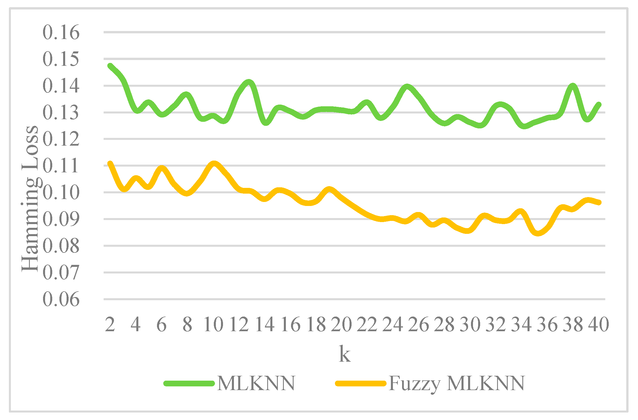
4.4. Comparative Analysis of Fuzzy MLKNN with MLKNN

According to the above parameter settings, two sets of comparative experiments are carried out on the preprocessed data set to observe the performance under different K values and compare the advantages and disadvantages of the traditional algorithm and the improved algorithm. The results are shown in Figure 1, Figure 2, Figure 3, Figure 4 and Figure 5.
The smaller the HammingLoss, the smaller the average number of misclassifications, and therefore the better the performance. From Figure 1, it can be directly seen that the HammingLoss value of the improved algorithm has an overall improvement compared with the traditional algorithm. The HammingLoss value of the traditional algorithm is between 0.12 and 0.15, and the mean value is 0.132. The overall fluctuation is relatively stable, and the distribution of the smallest HammingLoss value is not obvious, which is obtained at K = 14, 28, 31, and 34, respectively. The HammingLoss value of the improved algorithm is between 0.08 and 0.11, with an average value of 0.096. During the change from K = 10 to 35, the overall trend decreases. The smallest HammingLoss value can be easily obtained from the figure at K = 35. At the same time, we can find that the algorithm’s performance before and after the improvement in HammingLoss is not synchronous with the variation of the K value. From the perspective of HammingLoss only, the value of K selected for the optimal performance of the traditional algorithm and the improved algorithm is different.
The higher the Average_Precision, the better the performance of the multi-label learning algorithm. It can be observed from Figure 2 that the Average_Precision of the improved algorithm is significantly better than the traditional algorithm, and the gap between the two becomes more obvious with the increase of the K value. The value of Average_Precision of the traditional algorithm is between 0.89 and 0.92, with an average value of 0.909, and as the value of K increases, the overall trend decreases. The algorithm performs best when K = 14. The value of Average_Precision of the improved algorithm is between 0.92 and 0.95, with a mean value of 0.938, and with the increase of the K value, the overall trend is upward. When the value of K takes a value near 36, the performance is optimal, and when K = 36, the value of Average_Precision is at most 0.944.
Since Rankingloss and OneError are considered indicators based on the order of labels and are in the same order of magnitude, the smaller the two indicators are, the better the performance is. This paper considers these two indicators at the same time. In Figure 3, the blue line is the RankingLoss with MLKNN, and in Figure 4, the green columnar presents OneError values with MLKNN. Respectively, the red line in Figure 3 and the orange columnar in Figure 4 are the RankingLoss and OneError values of Fuzzy MLKNN.
First of all, from the value of RankingLoss, the improved algorithm is better than the traditional algorithm, and as the value of k increases, this advantage is gradually obvious. The average value of the traditional algorithm on RankingLoss is 0.08, and the low values are obtained at K = 8, 11, and 14. The mean RankingLoss of the improved algorithm is 0.055, and the minimum value is obtained at K= 36. Secondly, from the perspective of the OneError value, it can be seen from the figure that the OneError value of the traditional algorithm is significantly higher than that of the improved algorithm, and the former value fluctuates greatly. The average OneError value of the traditional algorithm is 0.063, while the average OneError value of the improved algorithm is 0.016. Based on the consideration of the OneError value, the optimal K value of the traditional algorithm is obtained when K = 14; the optimal K value of the improved algorithm is obtained when K = 17.
Figure 5 shows the performance of Coverage under different K values. Coverage is the step size required to traverse the correct label. The smaller the index, the better the performance. From the figure, we can see that the Coverage of the improved algorithm is also significantly lower than that of the traditional algorithm. The mean value of the improved algorithm on Coverage is 2.585, and the traditional algorithm is 2.822. The minimum Coverage values of the improved algorithm can be obtained at 24~26, 36, while the minimum Coverage values of the traditional algorithm are obtained at 10, 11, and 14.
Through the analysis of the above experimental results, we find that the improved algorithm is better than the traditional algorithm in all evaluation metrics, and the performance of the OneError value is the most significant, proving that the fuzzy distance measure is effective in the multi-label learning process of credit data. In addition, through the analysis of the optimal selection of the K value on different indicators, this paper finds that the traditional algorithm and the improved algorithm are not consistent in the selection of the optimal K value. The selection of the optimal K value of the traditional algorithm is significantly lower than the improved algorithm. From the comprehensive consideration of the performance of the above five indicators, it is more appropriate to take 14 for the optimal K value of the traditional algorithm. And the optimal K value of the improved algorithm is 36. Therefore, for these two results, we mainly use the improved algorithm with better performance in the following analysis process and select the K value of 36 to conduct further in-depth research on the data.

5. User Portrait

To make a portrait of users, we need to describe the distribution characteristics of labels. Referring to [50,51], we choose the best parameter with Fuzzy MLKNN, K = 36, and then conduct the algorithm with the whole dataset. The results are shown in Table 6 and Figure 6. Table 6 summarizes the proportion of one label, and Figure 6 describes user labels.
Firstly, from the learning results of one label in Table 9, users with low credit frequency account for the largest proportion, accounting for about 73%, followed by users with relatively stable personal development, accounting for about 67%, and the third is users with low credit concerns account for about 47%. It is more consistent with the actual situation. Most credit users have a low frequency of credit activities. The proportion of users with a medium frequency of credit activities is the least, indicating that the polarization of credit users is more serious in terms of credit activities.
Secondly, from the learning results of user labels, the proportion of credit users with predicted labels [136], [236], and [137] reached 59%, accounting for more than half of the total number of credit users, similar to the actual life situation. The user group represented by [136] has stable personal development, low credit frequency, and low credit concern. These users account for about 30% of the total number of users. [236] represents groups with unstable personal development, low credit frequency, and low credit concern, accounting for about 17% of the total users. From this, we can find that there is no significant correlation between the personal stability status and the credit status of credit reporting users to a certain extent. [137] represents groups with stable personal development, low credit frequency, and moderate credit concern, accounting for about 12% of the total population. The fourth and fifth place are [158] and [237], respectively, representing groups with stable personal development, high credit frequency, and high credit status concern, and individuals with unstable personal development, low credit frequency, and medium credit concern. This result also verifies the earlier conclusion that an individual’s stability does not directly affect his credit status. In addition, we also found a relationship between the frequency of credit activities and attention to the credit situation. High credit frequency is accompanied by high credit attention, while low and medium credit frequency also pays less attention to credit status, which aligns with real life.

6. Conclusions

This paper proposes a systematic clustering algorithm–Fuzzy MLKNN, which uses intuitionistic fuzzy sets to conduct distance metrics, and then improves the MLKNN multi-label learning algorithm. From the experiments, we find it has three advantages over the classical algorithm. Firstly, by fuzzing the data, the subjectivity of the original data in the process of data discretization can be weakened, and the objectivity and authenticity of the experimental data can be enhanced simultaneously. Secondly, the classical algorithm is improved by using the Euclidean fuzzy distance formula; to a certain extent, the distance between sample points is more representative than the original distance. Third, the fuzzy-improved algorithm outperforms the classical algorithm in multiple performance indicators, among which the OneError indicator is the most obvious.
The limitation of this paper is that it only considers the advantages of the improved algorithm from an experimental point of view and has not yet obtained relevant theoretical proof. Therefore, some questions worthy of further study remain. Theoretical analysis concerning the effectiveness of Fuzzy MLKNN will need more discussion. Moreover, as with other multi-label algorithms, Fuzzy MLKNN may suffer from missing labels and noisy labels, which will need more data to test.

Author Contributions

Conceptualization, Z.Z. and L.H.; methodology, Z.Z.; software, Z.Z.; validation, Z.Z., L.H. and M.C.; formal analysis, L.H.; investigation, L.H.; resources, L.H.; data curation, L.H.; writing—original draft preparation, Z.Z.; writing—review and editing, Z.Z. and L.H.; visualization, M.C.; supervision, L.H.; project administration, L.H.; funding acquisition, L.H. All authors have read and agreed to the published version of the manuscript.

Funding

This research was funded by the National Natural Science Foundation of China (grant number: 72101279).

Data Availability Statement

The data will be open on Researchgate, the link is https://www.researchgate.net/profile/Lu-Han-57.

Acknowledgments

The work was supported by the National Natural Science Foundation of China (Grant No. 72101279).

Conflicts of Interest

The authors declare no conflict of interest.

Appendix A

  • function [Prior,PriorN,Cond,CondN]=MLKNN_train(train_data,train_target,Num,Smooth)
  • %MLKNN_train trains a multi-label k-nearest neighbor classifier
  • %
  • %    Syntax
  • %
  • %       [Prior,PriorN,Cond,CondN]=MLKNN_train(train_data,train_target,num_neighbor)
  • %
  • %    Description
  • %
  • %       KNNML_train takes,
  • %           train_data   - An MxN array, the ith instance of training instance is stored in train_data(i,:)
  • %           train_target - A QxM array, if the ith training instance belongs to the jth class, then train_target(j,i) equals +1, otherwise train_target(j,i) equals -1
  • %           Num          - Number of neighbors used in the k-nearest neighbor algorithm
  • %           Smooth       - Smoothing parameter
  • %      and returns,
  • %          Prior        - A Qx1 array, for the ith class Ci, the prior probability of P(Ci) is stored in Prior(i,1)
  • %           PriorN       - A Qx1 array, for the ith class Ci, the prior probability of P(~Ci) is stored in PriorN(i,1)
  • %           Cond         - A Qx(Num+1) array, for the ith class Ci, the probability of P(k|Ci) (0<=k<=Num), i.e., k nearest neighbors of an instance in Ci will belong to Ci, is stored in Cond(i,k+1)
  • %           CondN        - A Qx(Num+1) array, for the ith class Ci, the probability of P(k|~Ci) (0<=k<=Num), i.e., k nearest neighbors of an instance not in Ci will belong to Ci, is stored in CondN(i,k+1)
  •  
  •     [num_class,num_training]=size(train_target);
  •  
  • %Computing distance between training instances
  • dist_matrix=diag(realmax*ones(1,num_training));               
  •     for i=1:num_training-1
  •         if(mod(i,100)==0)
  •             disp(strcat('computing distance for instance:',num2str(i)));
  •         end
  •         vector1=train_data(i,:);
  •         for j=i+1:num_training            
  •             vector2=train_data(j,:);
  •             dist_matrix(i,j)=sqrt(sum((vector1-vector2).^2));
  •             dist_matrix(j,i)=dist_matrix(i,j);
  •         end
  •     end
  •     
  • %Computing Prior and PriorN
  •     for i=1:num_class
  •         temp_Ci=sum(train_target(i,:)==ones(1,num_training));         
  •         Prior(i,1)=(Smooth+temp_Ci)/(Smooth*2+num_training);
  •         PriorN(i,1)=1-Prior(i,1);
  •     end
  •  
  • %Computing Cond and CondN
  •     Neighbors=cell(num_training,1); %Neighbors{i,1} stores the Num neighbors of the ith training instance
  •     for i=1:num_training
  •         [temp,index]=sort(dist_matrix(i,:));
  •         Neighbors{i,1}=index(1:Num);
  • end                            
  •   
  • temp_Ci=zeros(num_class,Num+1);
  •     temp_NCi=zeros(num_class,Num+1);
  •     for i=1:num_training
  •         temp=zeros(1,num_class); 
  •         neighbor_labels=[];
  •         for j=1:Num
  •             neighbor_labels=[neighbor_labels,train_target(:,Neighbors{i,1}(j))];
  •         end
  •         for j=1:num_class
  •             temp(1,j)=sum(neighbor_labels(j,:)==ones(1,Num));                       
  • end
  •         for j=1:num_class
  •             if(train_target(j,i)==1)
  •                 temp_Ci(j,temp(j)+1)=temp_Ci(j,temp(j)+1)+1;
  •             else
  •                 temp_NCi(j,temp(j)+1)=temp_NCi(j,temp(j)+1)+1;
  •             end
  •         end
  •     end
  •     for i=1:num_class
  •         temp1=sum(temp_Ci(i,:));
  •         temp2=sum(temp_NCi(i,:));
  •         for j=1:Num+1
  •             Cond(i,j)=(Smooth+temp_Ci(i,j))/(Smooth*(Num+1)+temp1);
  •             CondN(i,j)=(Smooth+temp_NCi(i,j))/(Smooth*(Num+1)+temp2);
  •         end
  •     end         
  •  
  • Function [HammingLoss,RankingLoss,OneError,Coverage,Average_Precision,Outputs,Pre_Labels]=MLKNN_test(train_data,train_target,test_data,test_target,Num,Prior,PriorN,Cond,CondN)
  • %MLKNN_test tests a multi-label k-nearest neighbor classifier.
  • %
  • %    Syntax
  • %
  • %       [HammingLoss,RankingLoss,OneError,Coverage,Average_Precision,Outputs,Pre_Labels]=MLKNN_test(train_data,train_target,test_data,test_target,Num,Prior,PriorN,Cond,CondN)
  • %
  • %    Description
  • %
  • %       KNNML_test takes,
  • %           train_data       - An M1xN array, the ith instance of training instance is stored in train_data(i,:)
  • %           train_target     - A QxM1 array, if the ith training instance belongs to the jth class, then train_target(j,i) equals +1, otherwise train_target(j,i) equals -1
  • %           test_data        - An M2xN array, the ith instance of testing instance is stored in test_data(i,:)
  • %           test_target      - A QxM2 array, if the ith testing instance belongs to the jth class, test_target(j,i) equals +1, otherwise test_target(j,i) equals -1
  • %           Num              - Number of neighbors used in the k-nearest neighbor algorithm
  • %           Prior            - A Qx1 array, for the ith class Ci, the prior probability of P(Ci) is stored in Prior(i,1)
  • %           PriorN           - A Qx1 array, for the ith class Ci, the prior probability of P(~Ci) is stored in PriorN(i,1)
  • %           Cond             - A Qx(Num+1) array, for the ith class Ci, the probability of P(k|Ci) (0<=k<=Num), i.e., k nearest neighbors of an instance in Ci will belong to Ci, is stored in Cond(i,k+1)
  • %           CondN            - A Qx(Num+1) array, for the ith class Ci, the probability of P(k|~Ci) (0<=k<=Num), i.e., k nearest neighbors of an instance not in Ci will belong to Ci, is stored in CondN(i,k+1)
  • %      and returns,
  • %           HammingLoss      - The hamming loss on testing data
  • %           RankingLoss      - The ranking loss on testing data
  • %           OneError         - The one-error on testing data as
  • %           Coverage         - The coverage on testing data as
  • %           Average_Precision- The average precision on testing data
  • %           Outputs          - A QxM2 array, the probability of the ith testing instance belonging to the jCth class is stored in Outputs(j,i)
  • %           Pre_Labels       - A QxM2 array, if the ith testing instance belongs to the jth class, then Pre_Labels(j,i) is +1, otherwise Pre_Labels(j,i) is -1
  •  
  •     [num_class,num_training]=size(train_target);
  •     [num_class,num_testing]=size(test_target);
  •     
  • %Computing distances between training instances and testing instances
  •     dist_matrix=zeros(num_testing,num_training);
  •     for i=1:num_testing
  •         if(mod(i,100)==0)
  •             disp(strcat('computing distance for instance:',num2str(i)));
  •         end
  •         vector1=test_data(i,:);
  •         for j=1:num_training
  •             vector2=train_data(j,:);
  •             dist_matrix(i,j)=sqrt(sum((vector1-vector2).^2));
  •         end
  •     end
  •  
  • %Find neighbors of each testing instance
  •     Neighbors=cell(num_testing,1); %Neighbors{i,1} stores the Num neighbors of the ith testing instance
  •     for i=1:num_testing
  •         [temp,index]=sort(dist_matrix(i,:));
  •         Neighbors{i,1}=index(1:Num);
  •     end
  •     
  • %Computing Outputs
  •     Outputs=zeros(num_class,num_testing);
  •     for i=1:num_testing
  • %         if(mod(i,100)==0)
  • %             disp(strcat('computing outputs for instance:',num2str(i)));
  • %         end
  •         temp=zeros(1,num_class); %The number of the Num nearest neighbors of the ith instance which belong to the jth instance is stored in temp(1,j)
  •         neighbor_labels=[];
  •         for j=1:Num
  •             neighbor_labels=[neighbor_labels,train_target(:,Neighbors{i,1}(j))];
  •         end
  •         for j=1:num_class
  •             temp(1,j)=sum(neighbor_labels(j,:)==ones(1,Num));
  •         end
  •         for j=1:num_class
  •             Prob_in=Prior(j)*Cond(j,temp(1,j)+1);
  •             Prob_out=PriorN(j)*CondN(j,temp(1,j)+1);
  •             if(Prob_in+Prob_out==0)
  •                 Outputs(j,i)=Prior(j);
  •             else
  •                 Outputs(j,i)=Prob_in/(Prob_in+Prob_out);      
  •             end
  •         end
  •     end
  •     
  • %Evaluation
  •     Pre_Labels=zeros(num_class,num_testing)
  •     for i=1:num_testing
  •         for j=1:num_class
  •             if(Outputs(j,i)>=0.5)
  •                 Pre_Labels(j,i)=1;
  •             else
  •                 Pre_Labels(j,i)=-1;
  •             end
  •         end
  •     end
  •     HammingLoss=Hamming_loss(Pre_Labels,test_target)
  •     RankingLoss=Ranking_loss(Outputs,test_target);
  •     OneError=One_error(Outputs,test_target);
  •     Coverage=coverage(Outputs,test_target);
  •     Average_Precision=Average_precision(Outputs,test_target);

References

  1. Chen, X. Empirical Research on the Early Warning of Regional Financial Risk Based on the Credit Data of Central Bank. Credit. Ref. 2022, 9, 17–24. [Google Scholar]
  2. Hou, S.Q.; Chen, X.J. Absence and Improvement of Legal Protection of Personal Credit Information Rights and Interests in the Era of Big Data. Credit. Ref. 2022, 9, 25–34. [Google Scholar]
  3. Chen, Y.H.; Wang, J.Y. The Rule of Law Applicable to the 2nd Generation Credit Information System under the Background of the Social Credit System. Credit. Ref. 2020, 38, 51–55. [Google Scholar]
  4. Li, Z. Research on the Development of Internet Credit Reference in China and the Supervision over It. Credit. Ref. 2015, 33, 9–15. [Google Scholar]
  5. Tian, K. Constructing the Market-oriented Individual Credit Investigation Ecosystem. China Financ. 2022, 8, 90–92. [Google Scholar]
  6. Han, L.; Su, Z.; Lin, J. A Hybrid KNN algorithm with Sugeno measure for the personal credit reference system in China. J. Intell. Fuzzy Syst. 2020, 39, 6993–7004. [Google Scholar] [CrossRef]
  7. Lessmann, S.; Baesens, B.; Seow, H.; Thomas, L.C. Benchmarking state-of-the-art classification algorithms for credit scoring: An update of research. Eur. J. Oper. Res. 2015, 247, 124–136. [Google Scholar] [CrossRef] [Green Version]
  8. Moscato, V.; Picariello, A.; Sperlí, G. A benchmark of machine learning approaches for credit score prediction. Expert Syst. Appl. 2021, 165, 113986. [Google Scholar] [CrossRef]
  9. Tarekegn, A.N.; Giacobini, M.; Michalak, K. A review of methods for imbalanced multi-label classification. Pattern Recognit. 2021, 118, 107965. [Google Scholar] [CrossRef]
  10. Song, D.; Vold, A.; Madan, K.; Schilder, F. Multi-label legal document classification: A deep learning-based approach with label-attention and domain-specific pre-training. Inf. Syst. 2022, 106, 101718. [Google Scholar] [CrossRef]
  11. Tandon, K.; Chatterjee, N. Multi-label text classification with an ensemble feature space. J. Intell. Fuzzy Syst. 2022, 42, 4425–4436. [Google Scholar] [CrossRef]
  12. Chen, D.; Rong, W.; Zhang, J.; Xiong, Z. Ranking based multi-label classification for sentiment analysis. J. Intell. Fuzzy Syst. 2020, 39, 2177–2188. [Google Scholar] [CrossRef]
  13. Gibaja, E.L.; Ventura, S. A Tutorial on Multi-Label Learning. Acm Comput. Surv. 2015, 47, 1–38. [Google Scholar] [CrossRef]
  14. Gui, X.; Lu, X.; Yu, G. Cost-effective Batch-mode Multi-label Active Learning. Neurocomputing 2021, 463, 355–367. [Google Scholar] [CrossRef]
  15. Mishra, N.K.; Singh, P.K. Feature construction and smote-based imbalance handling for multi-label learning. Inf. Sci. 2021, 563, 342–357. [Google Scholar] [CrossRef]
  16. Xu, X.; Shan, D.; Li, S.; Sun, T.; Xiao, P.; Fan, J. Multi-label learning method based on ML-RBF and laplacian ELM. Neurocomputing 2019, 331, 213–219. [Google Scholar]
  17. Tsoumakas, G.; Katakis, I.; Vlahavas, I. Mining Multi-Label Data. In Data Mining and Knowledge Discovery Handbook; Springer: Boston, MA, USA, 2009; pp. 667–685. [Google Scholar]
  18. Boutell, M.R.; Luo, J.; Shen, X. Learning multi-label scene classification. Pattern Recognit. 2004, 37, 1757–1771. [Google Scholar] [CrossRef] [Green Version]
  19. Read, J.; Pfahringer, B.; Holmes, G. Classifier chains for multi-label classification. Mach. Learn. 2011, 85, 333–359. [Google Scholar]
  20. Lango, M.; Stefanowski, J. What makes multi-class imbalanced problems difficult? An experimental study. Expert Syst. Appl. 2022, 199, 116962. [Google Scholar] [CrossRef]
  21. Ruiz Alonso, D.; Zepeda Cortes, C.; Castillo Zacatelco, H.; Carballido Carranza, J.L.; Garcia Cue, J.L. Multi-label classification of feedbacks. J. Intell. Fuzzy Syst. 2022, 42, 4337–4343. [Google Scholar] [CrossRef]
  22. Yapp, E.K.Y.; Li, X.; Lu, W.F.; Tan, P.S. Comparison of base classifiers for multi-label learning. Neurocomputing 2020, 394, 51–60. [Google Scholar] [CrossRef]
  23. Lv, S.; Shi, S.; Wang, H.; Li, F. Semi-supervised multi-label feature selection with adaptive structure learning and manifold learning. Knowl. Based Syst. 2021, 214, 106757. [Google Scholar] [CrossRef]
  24. Tan, A.; Liang, J.; Wu, W.; Zhang, J. Semi-supervised partial multi-label classification via consistency learning. Pattern Recognit. 2022, 131, 108839. [Google Scholar] [CrossRef]
  25. Li, Q.; Peng, X.; Qiao, Y.; Hao, Q. Unsupervised person re-identification with multi-label learning guided self-paced clustering. Pattern Recognit. 2022, 125, 108521. [Google Scholar] [CrossRef]
  26. Joachims, T. Optimizing search engines using clickthrough data. In Proceedings of the Eighth ACM SIGKDD International Conference on Knowledge Discovery and Data Mining KDD ’02, Edmonton, AB, Canada, 23–26 July 2002; ACM: New York, NY, USA, 2002; pp. 133–142. [Google Scholar] [CrossRef]
  27. Freund, Y.; Schapire, R.E. A Decision-Theoretic Generalization of On-Line Learning and an Application to Boosting. J. Comput. Syst. Sci. 1997, 55, 119–139. [Google Scholar] [CrossRef] [Green Version]
  28. Zhang, M.; Zhou, Z. ML-KNN: A lazy learning approach to multi-label learning. Pattern Recognit. 2007, 40, 2038–2048. [Google Scholar] [CrossRef]
  29. Zhu, D.; Zhu, H.; Liu, X.; Li, H.; Wang, F.; Li, H.; Feng, D. CREDO: Efficient and privacy-preserving multi-level medical pre-diagnosis based on ML-kNN. Inf. Sci. 2020, 514, 244–262. [Google Scholar] [CrossRef]
  30. Zhu, X.; Ying, C.; Wang, J.; Li, J.; Lai, X.; Wang, G. Ensemble of ML-KNN for classification algorithm recommendation. Knowl. Based Syst. 2021, 221, 106933. [Google Scholar] [CrossRef]
  31. Bogatinovski, J.; Todorovski, L.; Džeroski, S.; Kocev, D. Comprehensive comparative study of multi-label classification methods. Expert Syst. Appl. 2022, 203, 117215. [Google Scholar] [CrossRef]
  32. Syropoulos, A.; Grammenos, T. A Modern Introduction to Fuzzy Mathematics; John Wiley & Sons, Ltd.: Hoboken, NJ, USA, 2020; pp. 39–69. [Google Scholar]
  33. Dunn, J.C. A fuzzy relative of the ISODATA process and its use in detecting compact well-separated clusters. J. Cybern. 1973, 3, 32–57. [Google Scholar] [CrossRef]
  34. Wu, C.; Wang, Z. A modified fuzzy dual-local information c-mean clustering algorithm using quadratic surface as prototype for image segmentation. Expert Syst. Appl. 2022, 201, 117019. [Google Scholar] [CrossRef]
  35. Wu, Z.; Wang, B.; Li, C. A new robust fuzzy clustering framework considering different data weights in different clusters. Expert Syst. Appl. 2022, 206, 117728. [Google Scholar] [CrossRef]
  36. Wei, H.; Chen, L.; Chen, C.P.; Duan, J.; Han, R.; Guo, L. Fuzzy clustering for multiview data by combining latent information. Appl. Soft Comput. 2022, 126, 109140. [Google Scholar] [CrossRef]
  37. De Carvalho, F.D.A.T.; Lechevallier, Y.; de Melo, F.M. Relational partitioning fuzzy clustering algorithms based on multiple dissimilarity matrices. Fuzzy Sets Syst. 2013, 215, 1–28. [Google Scholar] [CrossRef]
  38. Vluymans, S.; Cornelis, C.; Herrera, F.; Saeys, Y. Multi-label classification using a fuzzy rough neighborhood consensus. Inf. Sci. 2018, 433–434, 96–114. [Google Scholar] [CrossRef]
  39. Zhao, X.; Nie, F.; Wang, R.; Li, X. Improving projected fuzzy K-means clustering via robust learning. Neurocomputing 2022, 491, 34–43. [Google Scholar] [CrossRef]
  40. Varshney, A.K.; Muhuri, P.K.; Danish Lohani, Q.M. PIFHC: The Probabilistic Intuitionistic Fuzzy Hierarchical Clustering Algorithm. Appl. Soft Comput. 2022, 120, 108584. [Google Scholar] [CrossRef]
  41. Zadeh, L.A. Fuzzy sets. Inf. Control. 1965, 8, 338–353. [Google Scholar] [CrossRef] [Green Version]
  42. Atanassov, K. Intuitionistic fuzzy sets. Fuzzy Sets Syst. 1986, 20, 87–96. [Google Scholar] [CrossRef]
  43. Li, G.Y.; Yang, B.R.; Liu, Y.H.; Cao, D.Y. Survey of data mining based on fuzzy set theory. Comput. Eng. Des. 2011, 32, 4064–4067+4264. [Google Scholar]
  44. Xu, Z.S. Intuitionistic Fuzzy Aggregation Operators. IEEE Trans. Fuzzy Syst. 2007, 15, 1179–1187. [Google Scholar]
  45. Zhang, Z.; Han, L.; Chen, M. Multi-label learning with user credit data in China based on MLKNN. In Proceedings of the 2nd International Conference on Information Technology and Cloud Computing (ITCC 2022), Qingdao, China, 20–22 May 2022; pp. 105–111. [Google Scholar]
  46. Zhang, C.; Li, Z. Multi-label learning with label-specific features via weighting and label entropy guided clustering ensemble. Neurocomputing 2021, 419, 59–69. [Google Scholar] [CrossRef]
  47. Hurtado, L.; Gonzalez, J.; Pla, F. Choosing the right loss function for multi-label Emotion Classification. J. Intell. Fuzzy Syst. 2019, 36, 4697–4708. [Google Scholar] [CrossRef]
  48. Shu, S.; Lv, F.; Yan, Y.; Li, L.; He, S.; He, J. Incorporating multiple cluster centers for multi-label learning. Inf. Sci. 2022, 590, 60–73. [Google Scholar] [CrossRef]
  49. Skryjomski, P.; Krawczyk, B.; Cano, A. Speeding up k-Nearest Neighbors classifier for large-scale multi-label learning on GPUs. Neurocomputing 2019, 354, 10–19. [Google Scholar] [CrossRef]
  50. Liu, B.; Blekas, K.; Tsoumakas, G. Multi-label sampling based on local label imbalance. Pattern Recognit. 2022, 122, 108294. [Google Scholar] [CrossRef]
  51. Lyu, G.; Feng, S.; Li, Y. Noisy label tolerance: A new perspective of Partial Multi-Label Learning. Inf. Sci. 2021, 543, 454–466. [Google Scholar] [CrossRef]
Figure 1. HammingLoss values under different K values.
Applsci 12 11342 g001
Figure 2. Average_Precision under different K values.
Applsci 12 11342 g002
Figure 3. RankingLoss under different K values.
Applsci 12 11342 g003
Figure 4. One Error under different K values.
Applsci 12 11342 g004
Figure 5. Coverage under different K values.
Applsci 12 11342 g005
Figure 6. The distribution of user labels.
Applsci 12 11342 g006
Table 1. Summary of advantages and disadvantages of multi-label learning algorithms.
AlgorithmDescriptionsAdvantagesDisadvantages
Binary Correlation (BR)Individual classifier for each labelSimpleIgnores label correlations
Label Power Set (LP) Each unique label set as a class identifierSimpleNot applicable to more labels
Chain of Classifiers (CC)Extension of BR, String two classifiers into a chain for learningConsider label correlationsPerformance depends on the order of classifiers in the chain
RankSVMImprovement to the traditional SVMPerformance improvementNot suitable for dealing with high-dimensional samples
ML-DTImprovement to the traditional DTPerformance improvementNot suitable for processing continuous variables, large samples, and multi-class data
MLKNNImprovement to the traditional KNNStrong applicability, Performance improvementIgnores label correlations
Table 2. Notation.
Table 2. Notation.
VariablesDescription
X Samples space
Y Labels space
x i Arbitrary i-th sample
α i Feature vector of xi. The elements in αi are composed of intuitionistic fuzzy numbers.
y i Label set of xi
L The label category vector
l Arbitrary single category label l L
N ( x ) The set of K nearest neighbors of x identified in the training set
C x ( l ) The number of sample with label l in neighbor set N ( x )
H 1 l the event that x has label l
H 0 l The event that x has not label l
E j l The event that, among the K nearest neighbors of x, there are exactly j instances with label l.
Table 3. Correlation matrices of some variables.
Coefficient of Correlation(1)(2)(3)(4)(5)(6)(7)(8)(9)(10)
(1) year_income10000.010.01000.040.03
(2) credit_over_amount010.020.03−0.02−0.03−0.02−0.02−0.01−0.02
(3) loan_over_amount00.0211−0.01−0.01−0.02−0.020−0.01
(4) total_over_amount00.0311−0.01−0.01−0.02−0.020−0.01
(5) bank_legal_org_num0.01−0.02−0.01−0.0110.990.940.940.580.64
(6) bank_org_num0.01−0.03−0.01−0.010.9910.930.930.590.65
(7) credit_legal_org_num0−0.02−0.02−0.020.940.93110.580.63
(8) credit_org_num0−0.02−0.02−0.020.940.93110.580.63
(9) total_credit_amount0.04−0.01000.580.590.580.5810.52
(10) query0.03−0.02−0.01−0.010.640.650.630.630.521
Table 4. Original dataset information.
ExamplesFeaturesLabels
traintestNominalNumericNumbersCardinalityDensityProportion
70030029830.3750.018
Table 5. Representative the credit variable data conversion process record.
Attribute NameData Conversion Process
educationPrimary school = 1; Secondary technical school = 2; Junior high school = 3; Senior middle school =4; Junior college = 5; University = 6; Postgraduate = 7
year_income1~10,000 RMB = 1; 10,001~50,000 RMB = 2; 50,001~100,000 RMB = 3; 100,001~500,000 RMB = 4; 500,001~1,000,000 RMB = 5; more than 1,000,000 RMB = 6
careerSoldier = 1; Heads of state agencies, party organizations, enterprises, and institutions = 2; Clerks and related personnel = 3; Production personnel in agriculture, forestry, animal husbandry, fishery, and water conservancy = 4; Commercial and service industry personnel = 5; Professional skill worker = 6; Production and transportation equipment operators and related personnel = 7
credit_account1~5 = 1; 6~10 = 2; 11~20 = 3; 21~50 = 4; more than 50 = 5;
loan_strokecount0~2 times = 1; 3~5 times = 2; 6~8 times = 3; 9~11 times = 4; more than 11 times = 5
total_credit_amount1~10,000 RMB = 1; 10,001~50,000 RMB = 2; 50,001~100,000 RMB = 3; 100,001~500,000 RMB = 4; 500,001~1,000,000 RMB = 5; More than 1,000,000 RMB = 6
total_use_amount1~10,000 RMB = 1; 10,001~50,000 RMB = 2; 50,001~100,000 RMB = 3; 100,001~500,000 RMB = 4; 500,001~1,000,000 RMB = 5; More than 1,000,000 RMB = 6
credit_amount_utilization_rate0~0.3 = 1; 0.3~0.6 = 2; 0.6~0.9 = 3; 0.9~1 = 4
query1~5 times = 1; 6~10 times = 2; 11~20 times = 3; 21~50 times = 4; 51~100 times = 5; more than 100 times = 6
credit_over_amountNo overdraft = 0; Overdraft = 1
total_over_amountNo overdue = 0; Overdue = 1
Table 6. Fuzzification process.
Attribute NameCorresponding Intuitionistic Fuzzy Number
education1:(0.01, 0.99); 2:(0.10, 0.90); 3:(0.17, 0.83); 4:(0.41, 0.59); 5:(0.79, 0.21); 6:(0.98, 0.02); 7(1, 0)
year_income1:(0.01, 0.99); 2:(0.40, 0.60); 3:(0.73, 0.27); 4:(0.95, 0.05); 5:(0.98, 0.02); 6:(1, 0)
credit_amount_utilization_rate1:(0.09, 0.91); 2:(0.20, 0.80); 3:(0.58, 0.42); 4:(0.97, 0.03); 5:(1, 0)
Table 7. Label information conversion process record.
Coding12345678
Labels NamePersonal development stabilityPersonal development instabilityLow frequency of credit activities Medium frequency of credit activitiesHigh frequency of credit activitiesLow attention to credit statusNormal attention to credit statusHigh attention to credit status
Table 8. Performance comparison between different multi-label algorithms.
Binary RelevanceClassifier ChainRank SVMFuzzy MLKNN
HammingLoss0.19470.25840.16880.0867
Average_Precision0.86520.75420.89440.9436
RankingLoss0.12810.24100.09000.0500
OneError0.08520.21300.06670.0133
Coverage3.05003.52002.99002.5267
Table 9. Proportion of one label.
Label CodeLabels NameProportion
1Personal development stability0.670
2Personal development instability0.330
3Low frequency of credit activities0.733
4Medium frequency of credit activities0.040
5High frequency of credit activities0.143
6Low attention to credit status0.470
7Medium attention to credit status0.260
8High attention to credit status0.173
Publisher’s Note: MDPI stays neutral with regard to jurisdictional claims in published maps and institutional affiliations.

