Article

Comparing OBIA-Generated Labels and Manually Annotated Labels for Semantic Segmentation in Extracting Refugee-Dwelling Footprints

Christian Doppler Laboratory for Geospatial and EO-Based Humanitarian Technologies (GEOHUM), Department of Geoinformatics—Z_GIS, Paris Lodron University of Salzburg, Schillerstrasse 30, 5020 Salzburg, Austria
*
Authors to whom correspondence should be addressed.
Appl. Sci. 2022, 12(21), 11226; https://doi.org/10.3390/app122111226
Submission received: 24 September 2022 / Revised: 1 November 2022 / Accepted: 3 November 2022 / Published: 5 November 2022
(This article belongs to the Special Issue Advanced Machine Learning and Scene Understanding in Images and Data)

Abstract

:
Refugee-dwelling footprints derived from satellite imagery are beneficial for humanitarian operations. Recently, deep learning approaches have attracted much attention in this domain. However, most refugees are hosted by low- and middle-income countries where accurate label data are often unavailable. The Object-Based Image Analysis (OBIA) approach has been widely applied to this task for humanitarian operations over the last decade. However, the footprints were usually produced urgently, and thus, include delineation errors. Thus far, no research discusses whether these footprints generated by the OBIA approach (OBIA labels) can replace manually annotated labels (Manual labels) for this task. This research compares the performance of OBIA labels and Manual labels under multiple strategies by semantic segmentation. The results reveal that the OBIA labels can produce IoU values greater than 0.5, which can produce applicable results for humanitarian operations. Most falsely predicted pixels source from the boundary of the built-up structures, the occlusion of trees, and the structures with complicated ontology. In addition, we found that using a small number of Manual labels to fine-tune models initially trained with OBIA labels can outperform models trained with purely Manual labels. These findings show high values of the OBIA labels for deep-learning-based refugee-dwelling extraction tasks for future humanitarian operations.

1. Introduction

Forcibly displaced people (FDP) refers to a group of people who leave their home or home region involuntarily due to conflicts, generalized violence, persecution, or human rights violations [1]. The global FDP population surpassed 100 million in mid-2022, which represents more than 1% of the global population [2]. Refugees, as an important category of FDP, refer to a group of people who are outside their home country and have received recognized mandates from the United Nations (UN) [3]. Approximately 86% of global refugees are hosted by low- and middle-income countries which usually cannot provide sufficient living space, medical services, food, water, and sanitation [4]. United Nations High Commissioner for Refugees (UNHCR) [5] together with many non-governmental organizations such as Médecins Sans Frontières (MSF, Doctors Without Borders in English) [6] have provided multiple humanitarian operations, including allocation and distribution of living resources and medical services to protect refugees.
Estimating the refugee population in need is essential for the logistics planning of humanitarian aid [7]. However, in most cases, it is difficult to collect such information in the field due to security and access reasons [8,9]. With the availability of very high spatial resolution satellite imagery, remote sensing has become one of the most powerful tools for population estimation for humanitarian operations over the last decade [8,10,11,12,13,14]. Refugee-dwelling footprints are useful in population estimation [15,16]. Therefore, producing high-quality refugee dwelling footprints efficiently can save much time for urgent humanitarian operations [17].
Multiple remote sensing image analysis techniques have been applied for this dwelling-extraction task during the last decade. Visual interpretation is thought to be capable of producing the refugee-dwelling footprints with the highest accuracy even though it still includes errors from inter-variability of observations [8]. However, it is labour-intensive and time-consuming [8]. Over the last decade, the OBIA approach has been widely applied to this task. Researchers have developed mature processing routines for producing refugee-dwelling footprints [18,19,20]. Nevertheless, due to the fast dynamics and diverse ontology of dwellings, the complexity and transferability of OBIA rulesets remain challenging [21].
In the past ten years, the development of deep learning in computer vision [22,23] has boosted a large number of applications in remote sensing [24,25,26]. However, related research for this extraction task is still limited. One main reason is the unavailability of adequate accurate label data of refugee dwellings [27] because most refugees are hosted by the countries where accurate label data of the footprints are not available in open sources, such as Open Street Map.
With the efforts of researchers and staff from humanitarian services at the Department of Geoinformatics Z_GIS, a large amount of label data for FDP dwellings has been produced by semi-automatic approaches (e.g., OBIA), with limited manual correction as post-processing [8]. Nevertheless, due to the urgency of the humanitarian operations, the produced OBIA labels may exhibit several types of annotation errors. Therefore, the OBIA label data are considered “noisy label data” compared with manually annotated label data (Manual labels). To the best of our knowledge, no research thus far has discussed whether we can make use of the generated tremendous OBIA labels to replace the Manual labels for this extraction task by deep learning approaches.
Currently, there are numerous deep learning models for remote-sensing-based building extraction tasks [28]. However, up to now, very few of them have been applied for this task. O. Ghorbanzadeh et al. [29] designed shallow convolutional neural networks (CNNs) to extract refugee dwellings in the Minawao refugee camp in northern Cameroon. The prediction results prove that CNNs have a high potential in this task. J. A. Quinn et al. [30] selected Mask-RCNN with ResNet-101 as a backbone to extract dwellings in multiple refugee camps. L. Wickert et al. [31] chose a Faster-RCNN model with ResNet-50 as a backbone to count dwellings in refugee camps. D. Tiede et al. [32] selected a Mask-RCNN model with ResNet-50 as a backbone to extract built-up structures in Khartoum in Sudan for fast humanitarian operations. G. W. Gella et al. [33] tested the spatial transferability of U-Net in this extraction task. G. W. Gella et al. [34] selected a Mask-RCNN model with ResNet-101 as a backbone to extract refugee dwellings in Cameroon. Y. Lu and C. Kwan [35] tested the performance of multiple neural networks and found that a fully neural network (FCN) outperforms Mask-RCNN in detecting refugee tents near the Syria–Jordan border.
On the basis of the findings from Y. Lu and C. Kwan [35], this research selected an FCN model for semantic segmentation for all experiments. Semantic segmentation can assign a class label to each pixel in an image to produce a fine-grained delineation of target objects with embedded spatial information [36] and has been proven to be robust in labelling noise in image analysis applications [37,38].
Up to now, many techniques have been developed to handle label noise in deep learning. Karimi et al. [39] reviewed related techniques and categorized them into six major classes, as shown in Figure 1. Recent progress in weakly supervised semantic segmentation (WSSS) enables CNNs to learn from weakly labelled data such as image-level annotations for semantic segmentation tasks. Related techniques such as self-supervised equivariant attention mechanism [40], group-wise learning [41], regional semantic contrast and aggregation [42], and adaptive early-learning correction [43] for WSSS also bring high value to make the best of the OBIA label data for refugee dwelling extraction tasks.
Among all techniques, intermixing training data from multiple sources proved to be a less intuitive but effective approach to increase the robustness of deep learning models for image segmentation [39]. Touzani and Granderson [44] intermixed image data from multiple study sites, various dates, and/or different sensors and trained models with label data from the Microsoft building footprint dataset to extract building footprints from satellite imagery. The results reveal that intermixing training data from multiple sources can produce promising results despite label noise. Inspired by these findings, this research selected intermixing as the strategy to handle the label noise issue as a starting point.
Inspired by this idea, we selected data from two refugee camps (Kule and Nguenyyiel in Ethiopia) from a dry season and a wet season (seen in Section 2.1) and designed multiple intermixing strategies (seen in Section 2.5) to make the comparison between the OBIA labels and the Manual labels in extracting refugee-dwelling footprints from very high-spatial-resolution satellite imagery (Pléiades-1, seen in Section 2.2) by semantic segmentation (U-Net with ResNet-34 as a backbone, seen in Section 2.3). In addition, we used a small amount (i.e., 10%, 20%, 30%, 40%, and 50%) of the Manual labels to fine-tune models trained with the OBIA labels to verify whether we can use a smaller amount of the Manual labels and existing OBIA labels to achieve similar performance as that of the models purely trained with a large amount of the Manual labels (seen in Section 2.5).
The main contribution of this research is that we first prove the OBIA labels, even though they include delineation errors, have very high potential to replace the manual labels, to a certain extent, in extracting refugee-dwelling footprints. Additionally, fine-tuning models trained with the OBIA labels with a small amount of the Manual labels can outperform models trained with purely Manual labels. The currently available OBIA labels from the last decade’s humanitarian operations could be fuel for future deep-learning-based refugee-dwelling extraction tasks.

2. Materials and Methods

2.1. Study Sites

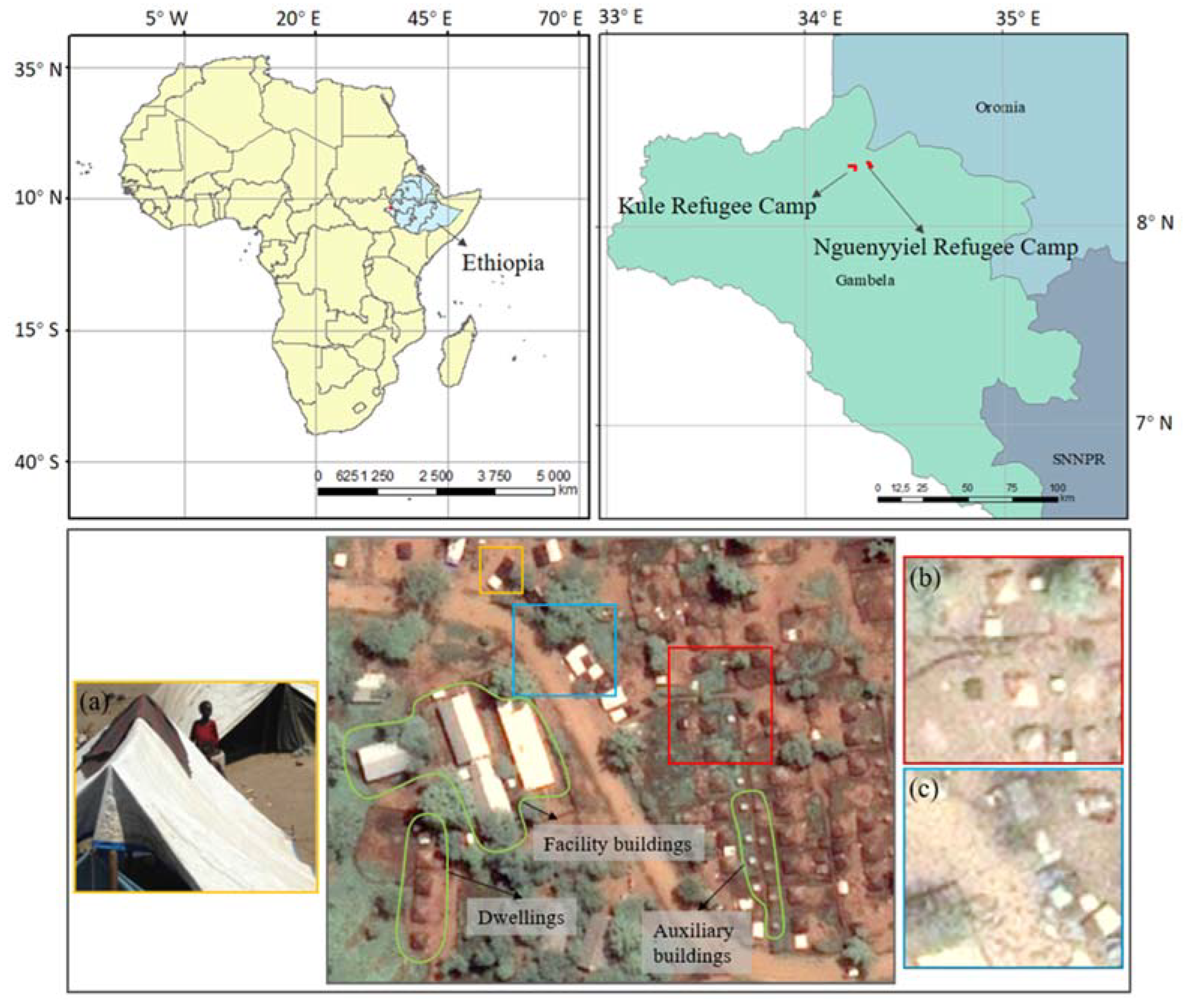
Kule and Nguenyyiel refugee camps are located in the Gambella region, Ethiopia. The Kule refugee camp was opened in 2014 in response to the major refugee influx from South Sudan and was fully occupied in 2016 [45]. The Nguenyyiel refugee camp was subsequently opened in 2016 to accommodate the influx of refugees from South Sudan due to the escalation of conflicts in July 2016 [46]. The location of the two camps together with the typical roof ontology of built-up structures can be found in Figure 2.
There are three main types of built-up structures in the two camps. Figure 2 shows several examples of the three types of built-up structures within the green boundary. The first type is for residential purposes, named dwellings. They are usually represented as white rectangles or squares with an area ranging from 20 to 40 m2 from satellite imagery. The roof ontology of refugee dwellings may be subject to change by local refugee behaviors. For example, they covered dark brown cloth on the rooftop, as shown in Figure 2a (yellow boundary). In addition, the ontology can be changed by naturally rusting or sand. Thus, we can observe many dwellings that have turned to brown from white, as seen in Figure 2b (red boundary). The second type is auxiliary buildings that are generally used for storage or latrines. Their areas are usually less than 10 m2. The last type is facility buildings, which are usually white, bluish, brownish, or greyish rectangles whose area is usually larger than 50 m2.
In Gambella, the wet season usually lasts from April to November, and the dry season spans from December to March [47]. The vegetation, especially trees, can occlude part of built-up structures on the ground, which brings difficulty to the refugee-dwelling extraction tasks. Figure 2c (blue boundary) shows an example where trees occluded built-up structures during the wet season.

2.2. Data Preparation

We chose satellite imagery from the Pléiades-1 sensor with a spatial resolution of 2 m. Considering the common size of dwellings (20 to 40 m2) in the selected sites, we pan-sharpened the imagery with the panchromatic band from the same source and resampled it to 0.5 m in GeoTIFF format to help the models learn more geometric features. Two retrieval dates represent the dry season (24 March 2017) and the wet season (22 June 2018), respectively. The pixel depth is 16-bit. RGB bands were selected because we found that three input bands with pretrained weights from ImageNet datasets outperform four bands during the preliminary phase. All satellite images use WGS1984 as the geographic coordinate system and UTM 36N as the projected coordinate system.
The OBIA labels of the two camps include only a small part of auxiliary buildings. To make a comparable and systematic comparison, we detect only facility buildings and dwellings in this research for both types of labels. While the footprints of dwellings can be used for population estimation [7], the footprints of facility buildings could be auxiliary information for humanitarian operators. Due to the limited number of facility buildings, they can be easily deleted as well, if such information is not useful in operations. For these reasons, we use binary classes in this research, which are Target built-up structures, including both refugee dwellings and facility buildings, and Background.
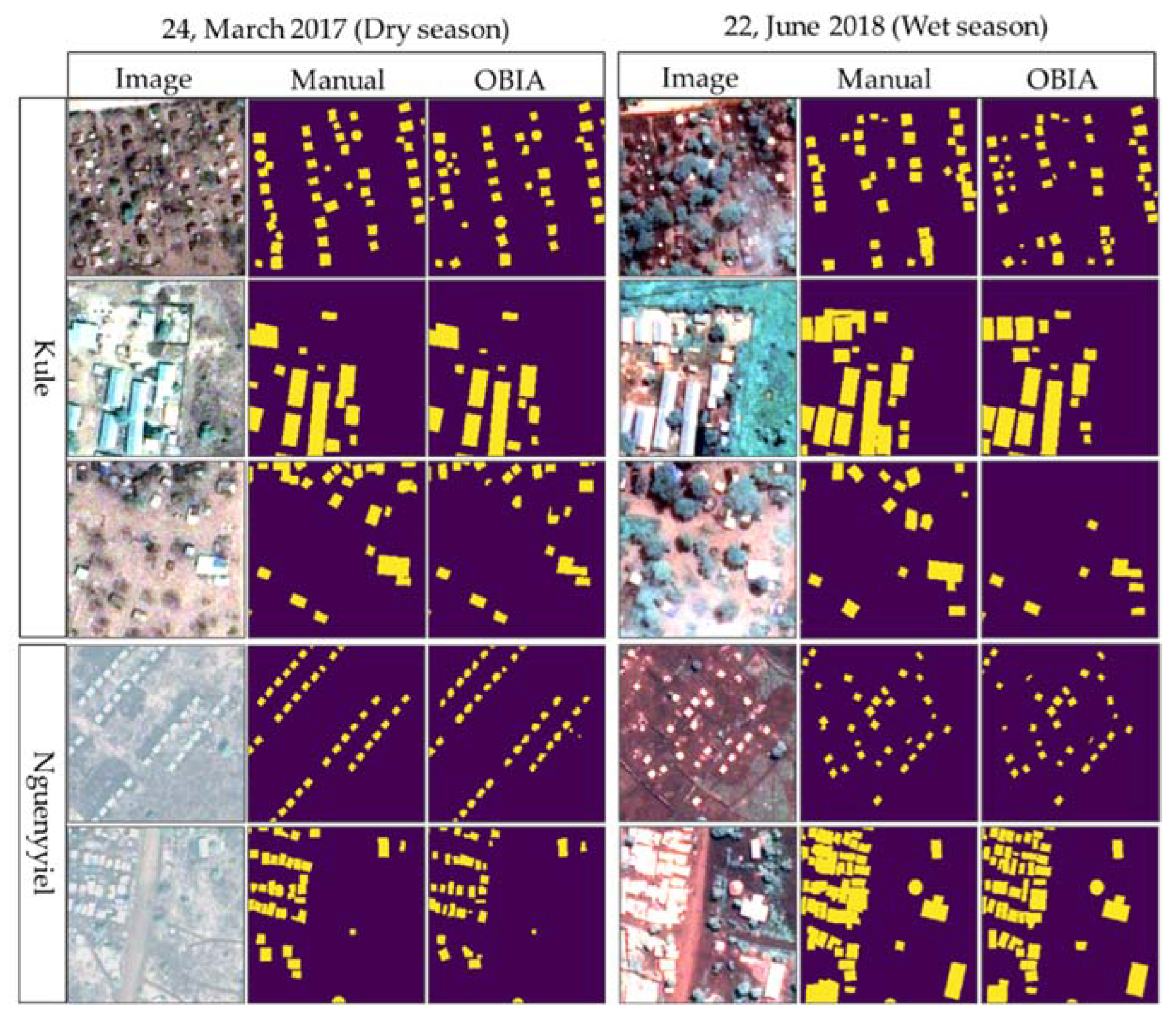
The OBIA labels were provided by the Department of Geoinformatics—Z_GIS of Paris Lodron University of Salzburg. Manual labels were manually annotated by one expert and crosschecked by another expert using a GIS software package. The annotated polygon data were converted to GeoTIFF format with a spatial resolution of 0.5 m. Figure 3 presents the built-up structures in two camps during two seasons together with the OBIA-generated labels and the Manual labels. We can observe the OBIA labels have high quality, in general, but include some annotation errors, such as missing some built-up structures.
During data preparation, we firstly selected areas for training (and validation) and testing. The dimensions of the selected areas were kept the same for each camp across two seasons. Secondly, the selected training (and validation) data were converted into patches with an overlap of 32 pixels in a shape of (128, 128) pixels. This patch size has been applied in related research and proved to be effective [33]. Thirdly, we deleted patches without any target built-up structures to reduce the redundancy of the class Background, in turn, to improve training speed and reduce the imbalance between the class Target built-up structures and the class Background. Following that, the produced patches were divided into training patches and validation patches at a ratio of 9:1. The data preparation process is briefly shown in Figure 4 below. Table 1 shows the number of training and validation patches for the OBIA labels and the Manual labels.

2.3. Model Structures and Hyperparameters

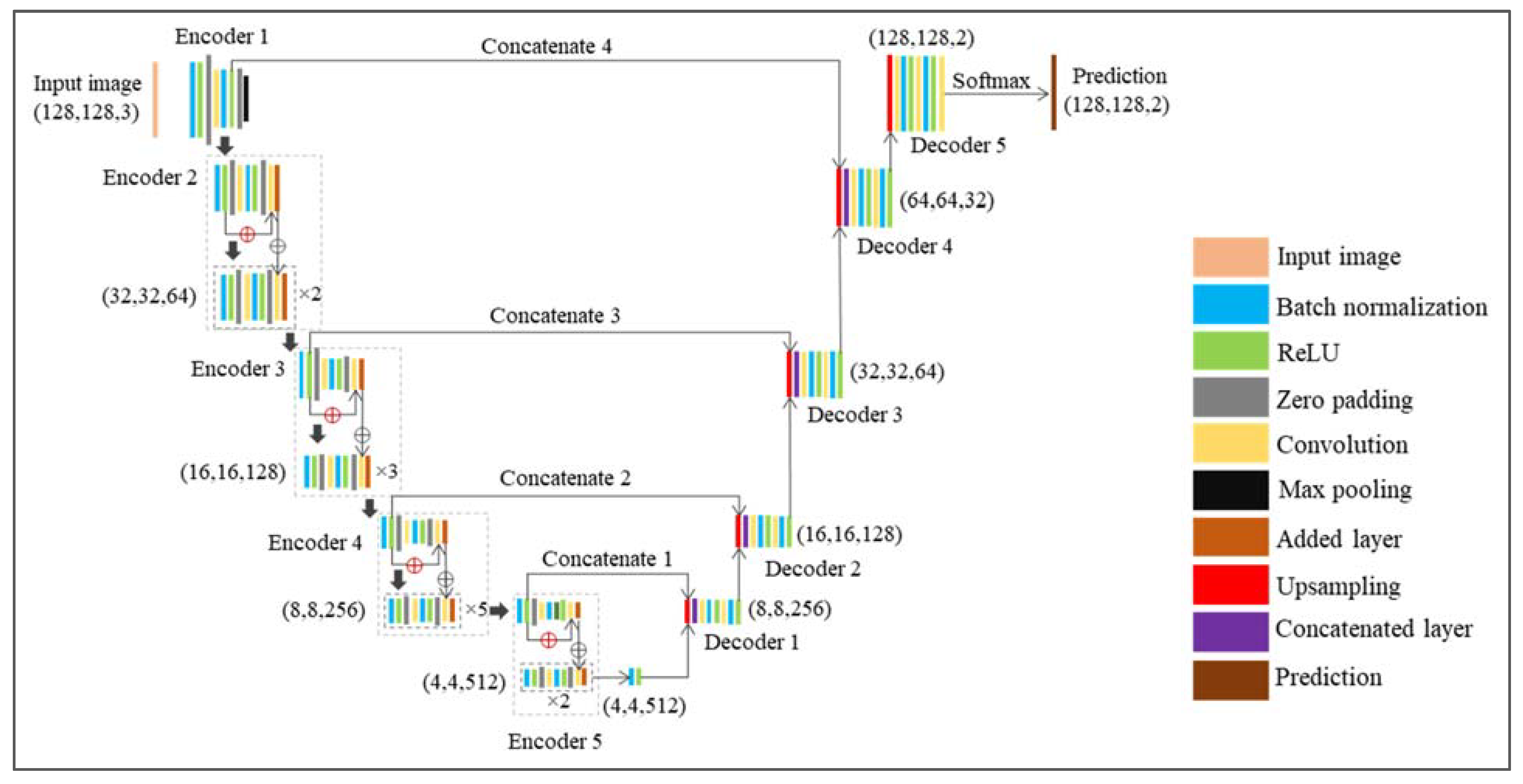
We selected U-Net [48] as an encoder–decoder structure with ResNet-34 [49] as a backbone (ResNet34-UNet) for all experiments. This architecture has been proven to work well in satellite image segmentation tasks [50].
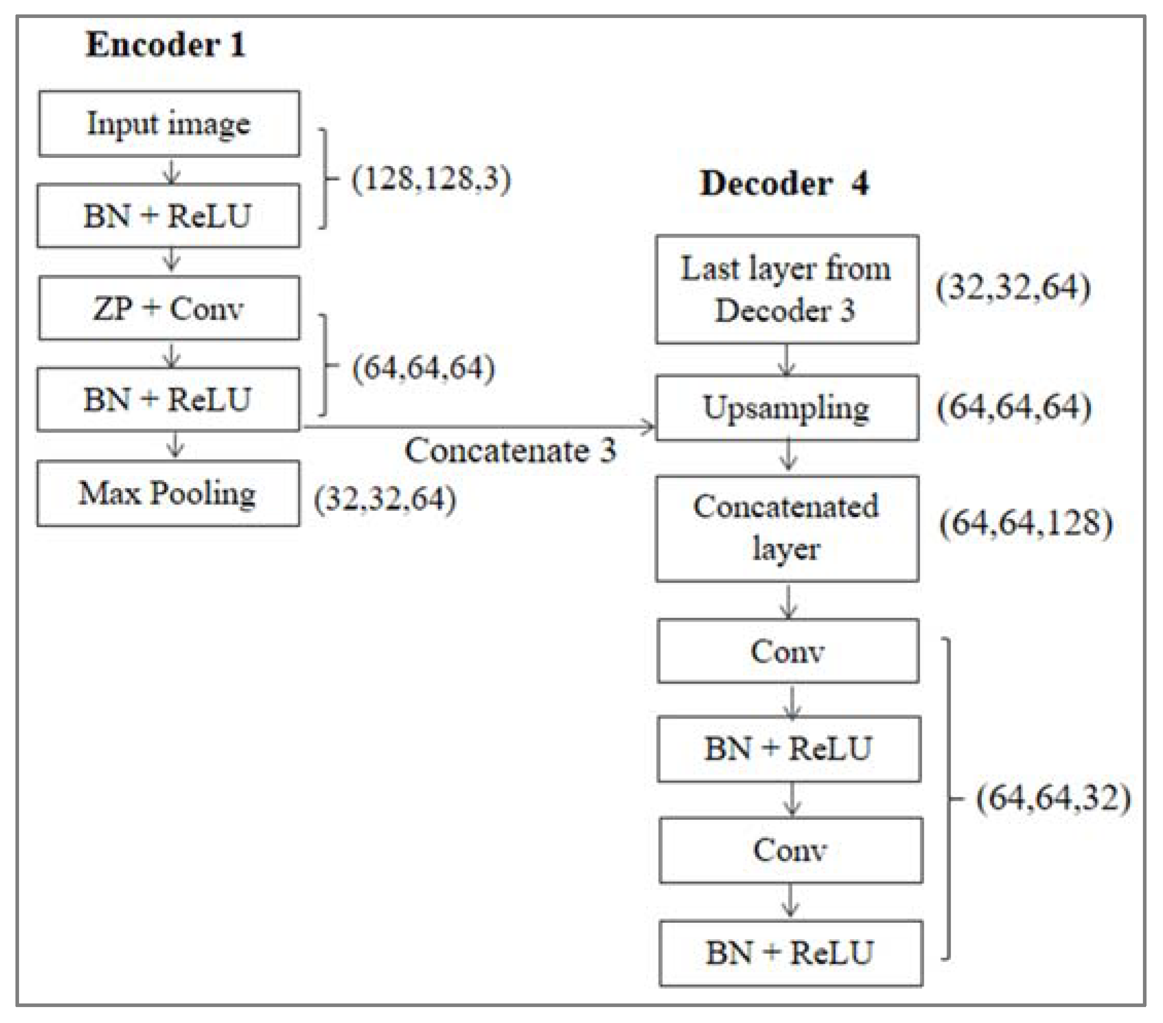
Figure 5 presents its general structure. Overall, there are five encoder units (Encoder 1, 2, 3, 4, and 5) and five decoder units (Decoder 1, 2, 3, 4, and 5) in ResNet34-UNet. Encoder 1 (seen in Figure 6) converts an input image with a shape of (128, 128, 3) to a set of feature maps with a shape of (32, 32, 64) after a batch normalization (BN) layer, an activation layer, a zero-padding (ZP) layer, a convolution (Conv) layer, a second BN layer, and an activation layer together with a max-pooling layer. The output of the second ReLU layer will be connected to the first layer of Decoder 4. Here, we used rectified linear unit (ReLU) as the activation function. Encoders 2, 3, 4, and 5 are residual units, and they share the same basic structure as Encoder 1.
Decoders 1, 2, 3, and 4 share similar structures. Figure 6 shows the structure of Decoder 4. It starts from an upsampling layer converting the shape of the input layer from (32, 32, 64) to (64, 64, 64). Then, it will be concatenated with the output of the first ReLU layer. After that, the first Conv layer reduces the number of features from 128 to 32. Encoder 5 uses a convolution layer to replace a concatenation layer and then connects to a SoftMax operation in the end to produce prediction results.

2.4. Accuracy Metrics

The performance of the proposed model was evaluated by Precision, Recall, and Intersection over Union (IoU) of target built-up structures, which have been widely applied in image analysis domains [51]. The calculation of the three metrics can be found in Equations (1)–(3) where TP, FP, and FN refer to the number of the True Positive, the False Positive, and the False Negative pixels for the semantic class. Additionally, we attached the results of F1-score and mean IoU in Appendix A, which can be helpful in comparison with outcomes from other related research in the future.
Precision = TP TP + FP
Recall = TP TP + FN
IoU = TP TP + FP + FN

2.5. The Designation of Experiments

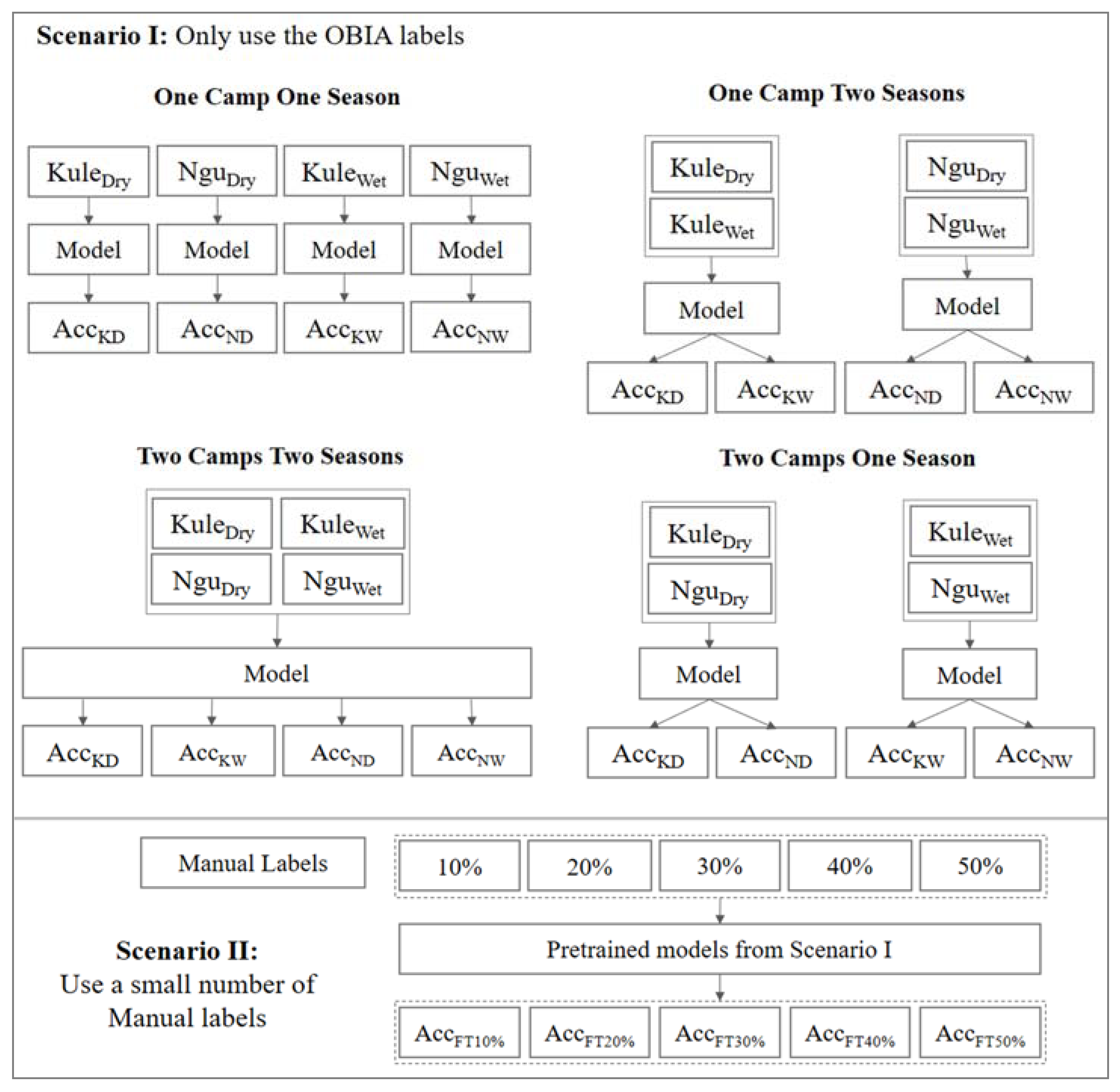
We designed two scenarios to compare the OBIA labels and the Manual labels. The designation of experiments for the two scenarios can be found in Figure 7.
In Scenario I, we designed four strategies to train models with the OBIA labels from past humanitarian operations. The first strategy is to train models with data from one camp and one season (OCOS). The other three training strategies include intermixing data from (1) one camp during two seasons (OCTS), (2) two camps during the same season (TCOS), and (3) two camps during two seasons (TCTS). The output results of Scenario I are expected to illustrate whether we can use existing OBIA-generated labels to replace the Manual labels. The three intermixing strategies may help reveal the influences of combining different data sources on the performance of the selected model.
In Scenario II, we randomly selected different percentages (10%, 20%, 30%, 40%, and 50%) of the total training patches of the Manual labels to fine-tune models pretrained by the four strategies in Scenario I. The reason that we made a random selection rather than a manual selection of patches with a high density of target built-up structures was to keep the data distribution of fine-tuning data similar to that of the training and testing data. The output results from Scenario II are expected to reveal whether we can use a smaller amount of the Manual labels based on models pretrained by the OBIA labels to replace a large number of the Manual labels.
Additionally, we designed baseline experiments where models were trained with purely Manual labels by the same strategies in Scenario I. The results from the two scenarios for the OBIA labels were compared with the performance of the baseline models for each camp during each season.

2.6. Set-Up

In this research, the ResNet34-UNet was implemented based on the Segmentation Model Python library [52]. For all experiments, we selected a batch size of 32, the Adam optimizer [53], and the Binary Cross Entropy as a loss function. We chose pretrained weights from ImageNet as initial weights. We used NVIDIA RTX3090 GPU to train and test models for all experiments in TensorFlow 2.7.0 environment. In terms of learning rates, we trained models with 200 epochs and chose 4 × 10⁻⁴ as an initial learning rate with 2 × 10⁻⁶ as a decay rate in Scenario I. In Scenario II, each model was fine-tuned with 10 epochs with a fixed learning rate of 1 × 10⁻⁴. The selection of the learning rates was based on multiple tests during the primary phase of this research.

3. Results

Table 2, Table 3 and Table 4 show the IoU, Precision, and Recall values of all implemented experiments for the two scenarios, as shown in Figure 7. To simplify the text, we use Kule to replace the Kule refugee camp and Kule Dry (or Wet) to replace the Kule refugee camp during the dry (or wet) season. Nguenyyiel and Nguenyyiel Dry (or Wet) follow the same nomenclature. In addition, we use OBIA-OCOS models, and Manual-OCOS models to represent models trained with the OBIA labels and the Manual labels by the OCOS strategy, respectively. The other three strategies (OCTS, TCOS, and TCTS) follow the same nomenclature. The highest values of metrics for each camp and season by each training strategy are highlighted in blue. The highest values for each camp and season among all training strategies are highlighted in red.

3.1. Scenario I

In terms of IoU values, we can observe four main findings. Firstly, models trained with the Manual labels outperform models trained with the OBIA labels in both camps during both seasons under all four training strategies. Secondly, the accuracy differences in Kule cases are higher than those in the Nguenyyiel cases. For example, in the Kule Dry case, the OBIA-OCOS model can produce an IoU value of 0.5113, while it is 0.5857 for the Manual-OCOS model. However, for the Nguenyyiel Dry case, the IoU values of the OBIA-OCOS model and the Manual-OCOS model are 0.6051 and 0.6377, respectively. Thirdly, the IoU values from the wet season are higher than those from the dry season. For instance, the IoU values of the OBIA-OCOS model and the Manual-OCOS model in the Kule Wet case are 0.5539 and 0.6400, respectively, which are higher than the values (0.5113, 0.5857) from the dry season. Last but not least, we can observe that the changes in IoU values (within 0.01, in general) brought by the three intermixing strategies are insignificant for the Manual labels. For the OBIA labels, the TCTS intermixing strategy shows a stable but limited improvement (approximately 0.01). The other two intermixing strategies cannot consistently improve the model performance. Instead, they decrease the IoU values in most cases.
The Recall values share similar findings as the IoU values, as shown in Table 3. We can observe the TCTS intermixing strategy brings a consistent improvement (approximately 0.01) for the models trained with the OBIA labels, but the other two strategies harm the model performance in most cases.
For Precision values as shown in Table 4, we can observe that the OBIA labels outperform the Manual labels in Precision values in all implemented experiments. On the contrary, the Manual labels outperform the OBIA labels in terms of Recall. For instance, in the Nguenyyiel Wet case, the Precision values of the OBIA-OCOS model and the Manual-OCOS model are 0.8545 and 0.8147, respectively. However, the Recall values of the same two models are 0.6890 and 0.7638, respectively. This finding indicates that the annotation errors in the OBIA labels cause models to miss much of TP in prediction.
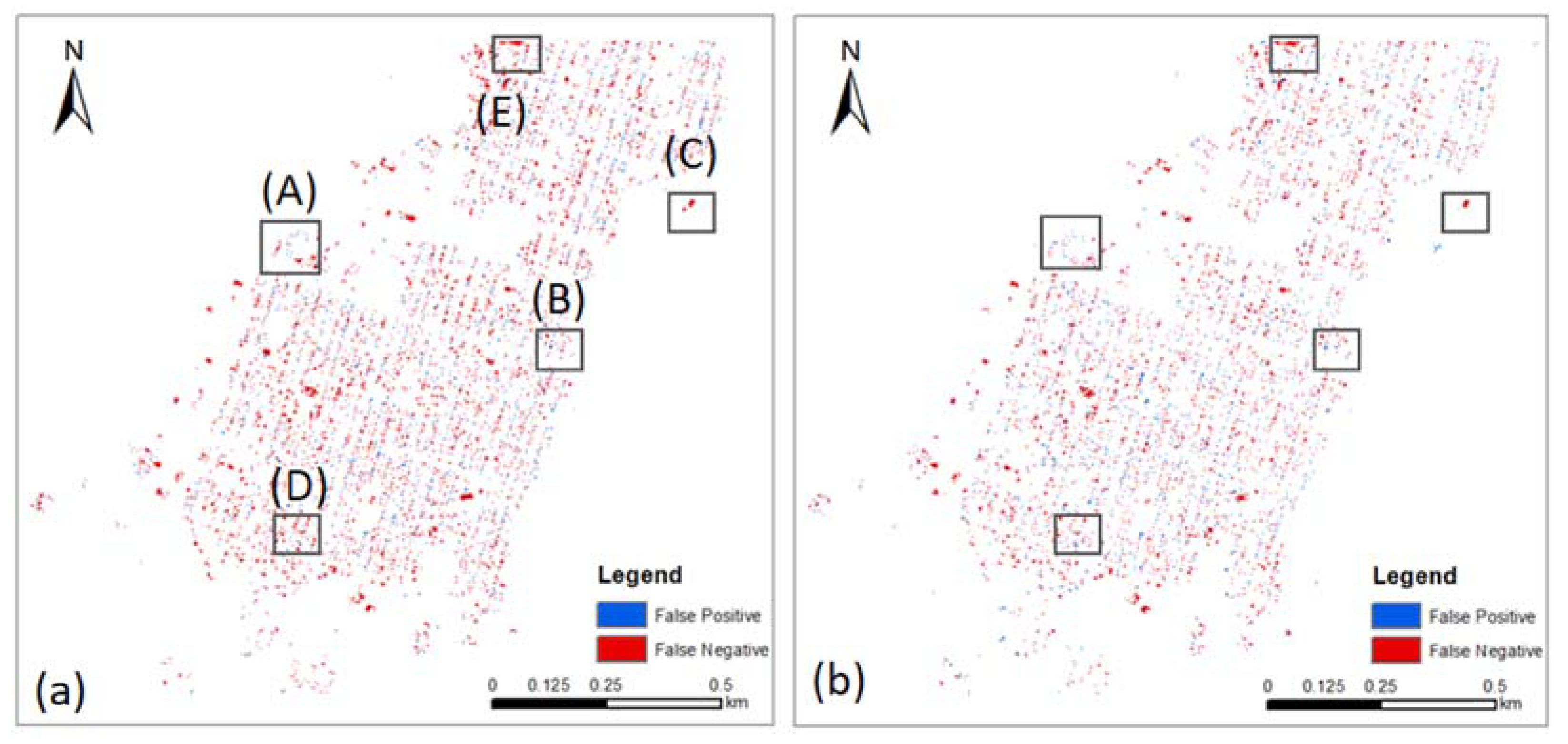
In the following content, we used Kule Wet as an example to explain the above findings because Kule Wet includes the most typical examples for an explanation. Figure 8 displays the spatial distribution of predicted FP (blue) and FN (red) pixels of the OBIA-OCOS model (left) and the Manual-OCOS model (right).
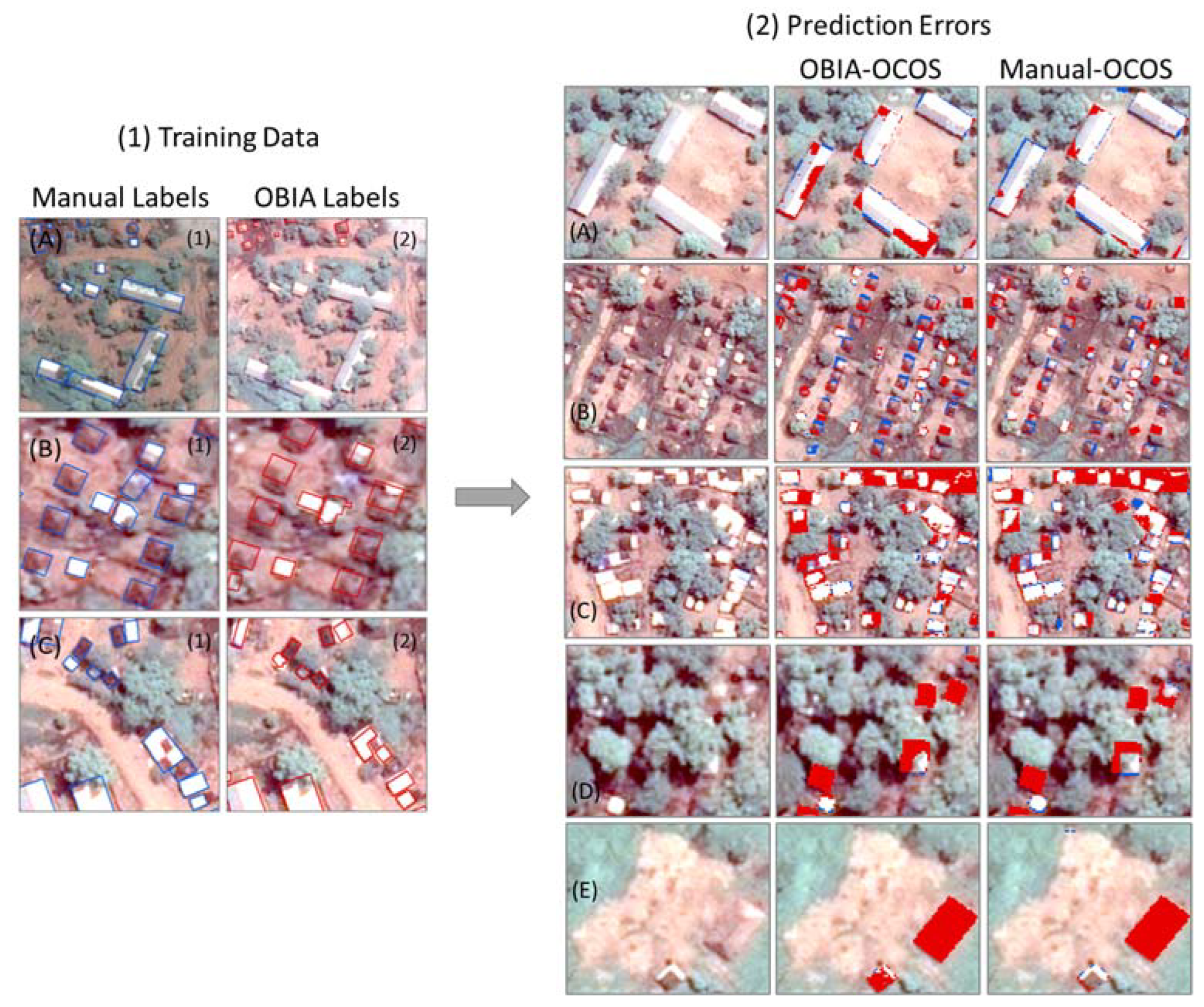
Overall, we can observe the two models share a similar spatial distribution of FP and FN pixels, but the OBIA-OCOS model produced more falsely predicted pixels. We selected five typical examples (A)–(E) to further show the prediction differences between the two models, as shown in Figure 9. In general, we found four main sources of errors coming from facility buildings, trees, boundaries, and brown cloth on the rooftop of dwellings.
There are two main types of facility buildings in the selected camps. Most facility buildings are white and grey in terms of spectral characteristics. Only a few of them are brownish. The OBIA labels missed some of the white and grey facility buildings in training data as shown in Figure 9(1A). This can be the reason that the Manual-OCOS models perform better than the OBIA-OCOS models for this type. For brownish facility buildings, both models cannot perform well, as shown in Figure 9(2E). This may be due to the very limited number of such structures in training data and the high similarity to the surrounding environment.
The occlusion of trees increases the difficulty of detecting target built-up structures. Both types of models cannot detect most brownish dwellings partially covered by trees, as shown in Figure 9(2D). However, due to the limited number of tree-occluded brownish dwellings, this type of error may not play a significant role in the results. Additionally, we can observe the IoU values from the wet season are higher than those from the dry season. This indicates that the similarity between target-up structures and the surrounding environment may play a more important role in this extraction task.
The prediction errors around the boundaries of target built-up structures widely spread the whole testing area for both models, as shown in Figure 8. Figure 9(1B) presents an example showing the difference in the annotation of dwellings between the OBIA labels and the Manual labels. We can observe an obvious shift of the OBIA labels compared with the Manual labels, which may cause more predicted FN and FP pixels. In addition, due to the difficulty of determining the exact boundaries of built-up structures, the Manual-OCOS models also unavoidably have FN and FP pixels around the boundaries. These incorrectly predicted pixels around the boundaries are the major source of errors at pixel levels for both types of labels. This type of error is also the main reason that the Manual labels outperform the OBIA labels in terms of IoU values.
Last but not least, models trained with either type of label are unable to detect brown cloth on the top of large dwellings that are densely distributed, as shown in Figure 9(2C). This is likely because both spatial distribution patterns (too dense) and the size (much larger) are different from most dwellings. However, for smaller dwellings covered by brown cloth, the Manual-OCOS models perform better than OBIA-OCOS models. This is mainly because the OBIA labels usually ignore brown parts within a dwelling and separate them into several individual dwellings, as shown in Figure 9(1C).

3.2. Scenario II

In Scenario II, we used different shares (10%, 20%, 30%, 40%, and 50%) of the Manual labels to fine-tune the models pretrained with the OBIA labels from Scenario I. The results reveal that the fine-tuning approach can produce a comparable or even better performance than the models trained with purely Manual labels. For example, the IoU value of the Manual-OCOS model for the Kule Dry is 0.5857. Fine-tuning the OBIA-OCOS model with 20% of the Manual labels improves the IoU value to 0.6033. The fine-tuned models produced all of the highest IoU values (highlighted in red) for each camp during each season. Based on the existing results, it is not found that intermixing training strategies are influential in the fine-tuning results. Additionally, most of the highest IoU values occur in between 20% and 40% of cleaned labels. However, no such stable percentage was found to perform the best in all cases. More research is required to dissect the further relations between these factors.

4. Discussion

This research aims to verify whether we can use the OBIA labels to replace the Manual labels with intermixing strategies (Scenario I), and, if the intermixing strategies fail, whether we can use a smaller number of Manual labels to reduce the manual annotation work (Scenario II) to achieve similar performance to a large number of Manual labels.
Touzani and Granderson [44] collected building footprints from open data web portals from 15 cities in America as label data for a semantic segmentation model (DeepLab-v3+). The collected labels, similar to the OBIA labels, include many annotation errors. The models trained with mixed datasets from 15 cities can produce a mean IoU value of 0.89. The finding shows the high value of using mixed open datasets from multiple sources to replace manually annotated labels for extracting building footprints. However, the performance of the OBIA labels was slightly improved only by the TCTS intermixing strategy. The other two intermixing strategies even slightly harmed the models. This is perhaps because we selected only two refugee camps. It may be worthwhile to intermix data from more refugee camps to verify whether the intermixing strategy can help improve this extraction task.
As mentioned in the Section 1, many techniques have been applied to handle label noise in deep learning. In this research, we found that the improvement of intermixing data from multiple sources is limited under the initial set up, but fine-tuning based on the models trained with intermixing data has very high potential.
In terms of the selection of networks, even though it is not the main focus of this research, we can nevertheless find that the selected model performs quite well compared with other models in previous research. G. W. Gella et al. [34] selected a Mask-RCNN model with ResNet-101 as a backbone to extract refugee dwellings in Cameroon. They used WorldView-3 and WorldView-2 images with a spatial resolution of 0.5 m, which is the same as that used in this research. The Mask-RCNN model produced the mean IoU value up to 0.669 which is lower than the outputs of all experiments here, as shown in Table A2 in Appendix A. These comparison results are consistent with the results from Y. Lu and C. Kwan [35]. In addition, Ref. [54] compared multiple semantic segmentation models, including three classical deep learning architectures (U-Net, LinkNet, and Feature Pyramid Network (FPN)) and twelve backbones (VGG16, VGG19, ResNet-18, ResNet-34, DenseNet-121, DenseNet-169, Inception-v3, InceptionResnet-v2, MobileNet-v1, MobileNet-v2, EfficientNet-B0, and EfficientNet-B1) to test the validity of the OBIA labels compared with the Manual labels by using the same training and testing data of the Kule refugee camp during the dry and the wet seasons. The results show that these models perform similarly, in general. Therefore, it is necessary to undertake more state-of-the-art techniques in the future to discover more suitable workflows for this task.

5. Conclusions

From this research, we found that the OBIA labels can help the models produce satisfying predicted labels with IoU values of target built-up structures greater than 0.5—even though the Manual labels still outperform the OBIA labels for each camp during each season. Intermixing the data from two camps and two seasons (TCTS) can slightly improve the performance of models trained with the OBIA labels. However, the other two strategies (OCTS and TCOS) cannot bring stable improvement and even sometimes harm the models. In addition, we found that both types of labels cannot properly detect brownish facility buildings, brownish dwellings partially occluded by trees, nor densely distributed large dwellings covered by brown cloth. The falsely predicted pixels around the boundary of target built-up structures may be the main source of prediction errors compared with other sources. Additionally, the reason that the Manual labels outperform the OBIA labels is mainly because the models trained with the Manual labels can produce fewer errors around the boundaries of structures. Additionally, it can be observed that the IoU values are higher during the wet season than during the dry season. This is likely because of the higher similarity between built-up structures and the surrounding environment during the dry season. Furthermore, we found fine-tuning models pretrained with the OBIA labels from Scenario I with smaller shares (10%, 20%, 30%, 40%, and 50%) of the Manual labels can enable the models to produce comparable or even better IoU values than the models trained with purely Manual labels.
These outcomes prove the remarkable potential of the OBIA labels to replace the Manual labels in future research. More research is required to make better use of the produced OBIA labels for future humanitarian operations.

Author Contributions

Conceptualization, Y.G., S.L. and D.T.; methodology and formal analysis, Y.G.; investigation, Y.G.; writing—original draft preparation, Y.G.; writing—review and editing, Y.G., S.L., D.T., G.W.G. and L.W. All authors have read and agreed to the published version of the manuscript.

Funding

This work was supported by Austrian Federal Ministry for Digital and Economic Affairs, the National Foundation for Research, Technology and Development, the Christian Doppler Research Association (CDG), and Médecins Sans Frontières (MSF) Austria.

Institutional Review Board Statement

Not applicable.

Informed Consent Statement

Not applicable.

Data Availability Statement

Those who are interested in the data can send data requests to [email protected]. The data will be provided pending approval of the request by Médecins Sans Frontières (MSF) Austria.

Conflicts of Interest

The authors declare no conflict of interest.

Appendix A

Table A1 and Table A2 present the results of F1-score and mean IoU values of all implemented experiments. The formula of the two metrics are shown in Equations (A1) and (A2).
F1-score = 2 × Precision × Recall Precision + Recall
  mIoU = 1 n k = 1 n TP ( TP + FP + FN )   ( n = 2 )
Table A1. The F1-score values of built-up structures of all implemented experiments.
Refugee CampSeasonTraining StrategyBaselineScenario IScenario II
ManualOBIA10%20%30%40%50%
KuleDryOCOS0.73870.67660.73650.75260.75150.74760.7499
OCTS0.73650.68440.73700.74420.74490.74670.7435
TCOS0.74110.69080.74340.74430.74420.74490.7443
TCTS0.74090.69070.72580.73790.73710.73940.7366
KuleWetOCOS0.78050.71290.77940.79080.79290.78140.7824
OCTS0.78490.70410.76450.77970.78390.77490.7814
TCOS0.77950.69050.78160.78560.78640.78740.7843
TCTS0.77590.71570.77270.77500.78640.78080.7778
NguenyyielDryOCOS0.77870.75400.77740.77990.78010.77970.7770
OCTS0.77960.75580.76000.77320.77860.77810.7779
TCOS0.77890.75390.77550.77830.77900.77930.7786
TCTS0.77990.75830.78040.78740.78580.78650.7835
NguenyyielWetOCOS0.78580.76510.78730.79070.78950.78730.7862
OCTS0.78530.76300.78680.78920.78920.78640.7844
TCOS0.78840.76290.79570.79780.79730.79600.7990
TCTS0.79770.77310.77530.76180.79690.77700.7955
Table A2. The mean IoU values of built-up structures of all implemented experiments.
Refugee CampSeasonTraining StrategyBaselineScenario IScenario II
ManualOBIA10%20%30%40%50%
KuleDryOCOS0.78190.74290.77950.79080.79000.78730.7888
OCTS0.78030.74810.78080.78530.78580.78690.7847
TCOS0.78340.75200.78490.78540.78530.78570.7852
TCTS0.78320.75180.77360.78130.78070.78210.7803
KuleWetOCOS0.81150.76640.81080.81860.82000.81190.8126
OCTS0.81450.76100.80050.81090.81390.80740.8120
TCOS0.81080.75280.81220.81510.81560.81620.8139
TCTS0.80820.76820.80610.80770.81550.81150.8094
NguenyyielDryOCOS0.81570.79930.81490.81650.81660.81630.8145
OCTS0.81630.80040.80300.81190.81560.81530.8151
TCOS0.81580.79920.81340.81540.81590.81610.8156
TCTS0.81640.80210.81690.82160.82050.82100.8189
NguenyyielWetOCOS0.81740.80330.81850.82080.81990.81840.8177
OCTS0.81700.80180.81820.81970.81980.81780.8163
TCOS0.81920.80190.82450.82590.82560.82460.8268
TCTS0.82580.80880.81020.80040.82520.81100.8242

References

  1. UNHCR. Global Trends: Forced Displacement in 2020; UNHCR Global Trends: Copenhagen, Denmark, 2021; p. 72. [Google Scholar]
  2. UNHCR. UNHCR: A Record 100 Million People Forcibly Displaced Worldwide. UN News, 23 May 2022. [Google Scholar]
  3. UNHCR. Persons Who are Forcibly Displaced, Stateless and Others of Concern to UNHCR, UNHCR The UN Refugee Agency. 2021. Available online: https://www.unhcr.org/refugee-statistics/methodology/definition/ (accessed on 28 November 2021).
  4. UNHCR. Mid-Year Trends 2021; UNCHR: Copenhagen, Denmark, 2021. [Google Scholar]
  5. Elizabeth, U.; Stuart, M. Report on UNHCR’s Response to COVID-19; UNCHR: Geneva, Switzerland, 2020. [Google Scholar]
  6. Médecins Sans Frontières. Global Migration and Refugee Crisis—Record Numbers of People Have Been Forced from Home and Struggle to Find Safety. 2021. Available online: https://www.doctorswithoutborders.org/refugees (accessed on 28 November 2021).
  7. Çelik, M.; Ergun, Ö.; Johnson, B.; Keskinocak, P.; Lorca, Á.; Pekgün, P.; Swann, J. Humanitarian logistics. In New Directions in Informatics, Optimization, Logistics, and Production; INFORMS: Catonsville, MD, USA, 2012; pp. 18–49. [Google Scholar]
  8. Lang, S.; Füreder, P.; Riedler, B.; Wendt, L.; Braun, A.; Tiede, D.; Schoepfer, E.; Zeil, P.; Spröhnle, K.; Kulessa, K.; et al. Earth observation tools and services to increase the effectiveness of humanitarian assistance. Eur. J. Remote Sens. 2020, 53, 67–85. [Google Scholar] [CrossRef] [Green Version]
  9. Kunz, N.; Van Wassenhove, L.N.; Besiou, M.; Hambye, C.; Kovacs, G. Relevance of humanitarian logistics research: Best practices and way forward. Int. J. Oper. Prod. Manag. 2017, 37, 1585–1599. [Google Scholar] [CrossRef]
  10. Witharana, C. Who Does What Where? Advanced Earth Observation for Humanitarian Crisis Management. In Proceedings of the 2012 IEEE 6th International Conference on Information and Automation for Sustainability, Beijing, China, 27–29 September 2012; pp. 1–6. [Google Scholar]
  11. Füreder, P.; Lang, S.; Hagenlocher, M.; Tiede, D.; Wendt, L.; Rogenhofer, E. Earth Observation and GIS to Support Humanitarian Operations in Refugee/IDP Camps. In Proceedings of the ISCRAM 2015—The 12th International Conference on Information Systems for Crisis Response and Management, Kristiansand, Norway, 24–27 May 2015. [Google Scholar]
  12. Lang, S.; Schoepfer, E.; Zeil, P.; Riedler, B. Earth observation for humanitarian assistance. GI Forum 2017, 1, 157–165. [Google Scholar] [CrossRef] [Green Version]
  13. Braun, A.; Hochschild, V. Potential and limitations of radar remote sensing for humanitarian operations. GI Forum 2017, 1, 1228–1243. [Google Scholar] [CrossRef]
  14. Lang, S.; Füreder, P.; Rogenhofer, E. Earth observation for humanitarian operations. In Yearbook on Space Policy 2016; Springer: Cham, Switzerland, 2018; pp. 217–229. [Google Scholar]
  15. Checchi, F.; Stewart, B.T.; Palmer, J.J.; Grundy, C. Validity and feasibility of a satellite imagery-based method for rapid estimation of displaced populations. Int. J. Health Geogr. 2013, 12, 4. [Google Scholar] [CrossRef] [Green Version]
  16. Spröhnle, K.; Tiede, D.; Schoepfer, E.; Füreder, P.; Svanberg, A.; Rost, T. Earth observation-based dwelling detection approaches in a highly complex refugee camp environment—A comparative study. Remote Sens. 2014, 6, 9277–9297. [Google Scholar] [CrossRef] [Green Version]
  17. Füreder, P.; Tiede, D.; Lüthje, F.; Lang, S. Object-based dwelling extraction in refugee/IDP camps–challenges in an operational mode. South-East. Eur. J. Earth Obs. Geomat. 2014, 3, 539–544. [Google Scholar]
  18. Kraffi, P.; Tiede, D.; Fureder, P. Template Matching to Support Earth Observation Based Refugee Camp Analysis in Obia Workflows—Creation and Evaluation of a Dwelling Template Library for Improving Dwelling Extraction Within an Object-Based Framework. In Proceedings of the GEOBIA 2016: Solutions and Synergies, Enschede, The Netherlands, 14–16 September 2016. [Google Scholar]
  19. Tiede, D.; Krafft, P.; Füreder, P.; Lang, S. Stratified template matching to support refugee camp analysis in OBIA workflows. Remote Sens. 2017, 9, 326. [Google Scholar] [CrossRef] [Green Version]
  20. Tiede, D.; Füreder, P.; Lang, S.; Hölbling, D.; Zeil, P. Automated analysis of satellite imagery to provide information products for humanitarian relief operations in refugee camps -from scientific development towards operational services. Photogramm. Fernerkund. Geoinf. 2013, 2013, 185–195. [Google Scholar] [CrossRef]
  21. Tiede, D.; Lang, S.; Hölbling, D.; Füreder, P. Transferability of Obia Rulesets for Idp Camp Analysis in Darfur. In Proceedings of the GEOBIA 2010: Geographic Object-Based Image Analysis, Ghent, Belgium, 29 June–2 July 2021. [Google Scholar]
  22. Voulodimos, A.; Doulamis, N.; Doulamis, A.; Protopapadakis, E. Deep Learning for Computer Vision: A Brief Review. Comput. Intell. Neurosci. 2018, 2018, 7068349. [Google Scholar] [CrossRef]
  23. Krizhevsky, A.; Sutskever, I.; Hinton, G.E. ImageNet Classification with Deep Convolutional Neural Networks. Adv. Neural Inf. Process. Syst. 2012, 25, 1097–1105. [Google Scholar] [CrossRef] [Green Version]
  24. Zhu, M.; He, Y.; He, Q. A Review of Researches on Deep Learning in Remote Sensing Application. Int. J. Geosci. 2019, 10, 1–11. [Google Scholar] [CrossRef] [Green Version]
  25. Zhang, L.; Zhang, L.; Kumar, V. Deep learning for Remote Sensing Data. IEEE Geosci. Remote Sens. Mag. 2016, 4, 22–40. [Google Scholar] [CrossRef]
  26. Zhu, X.X.; Tuia, D.; Mou, L.; Xia, G.S.; Zhang, L.; Xu, F.; Fraundorfer, F. Deep learning in remote sensing: A review. arXiv 2017, arXiv:1710.03959. [Google Scholar]
  27. Fisher, A.; Mohammed, E.A.; Mago, V. TentNet: Deep Learning Tent Detection Algorithm Using A Synthetic Training Approach. IEEE Trans. Syst. Man Cybern. Syst. 2020, 2020, 860–867. [Google Scholar]
  28. Luo, L.; Li, P.; Yan, X. Deep learning-based building extraction from remote sensing images: A comprehensive review. Energies 2021, 14, 7982. [Google Scholar] [CrossRef]
  29. Ghorbanzadeh, O.; Tiede, D.; Dabiri, Z.; Sudmanns, M.; Lang, S. Dwelling extraction in refugee camps using CNN—First experiences and lessons learnt. Int. Arch. Photogramm. Remote Sens. Spat. Inf. Sci. 2018, 42, 161–166. [Google Scholar] [CrossRef] [Green Version]
  30. Quinn, J.A.; Nyhan, M.M.; Navarro, C.; Coluccia, D.; Bromley, L.; Luengo-Oroz, M. Humanitarian applications of machine learning with remote-sensing data: Review and case study in refugee settlement mapping. Philos. Trans. R. Soc. A Math. Phys. Eng. Sci. 2018, 376, 20170363. [Google Scholar] [CrossRef] [Green Version]
  31. Wickert, L.; Bogen, M.; Richter, M. Lessons Learned on Conducting Dwelling Detection on VHR Satellite Imagery for the Management of Humanitarian Operations. Sens. Transducers 2021, 249, 45–53. [Google Scholar]
  32. Tiede, D.; Schwendemann, G.; Alobaidi, A.; Wendt, L.; Lang, S. Mask R-CNN based building extraction from VHR satellite data in operational humanitarian action: An example related to COVID-19 response in Khartoum, Sudan. Trans. GIS 2021, 25, 1213–1227. [Google Scholar] [CrossRef] [PubMed]
  33. Gella, G.W.; Wendt, L.; Lang, S.; Braun, A. Testing Transferability of Deep-Learning-Based Dwelling Extraction in Refugee Camps. GI Forum 2021, 9, 220–227. [Google Scholar]
  34. Gella, G.W.; Wendt, L.; Lang, S.; Tiede, D.; Hofer, B.; Gao, Y.; Braun, A. Mapping of Dwellings in IDP/Refugee Settlements from Very High-Resolution Satellite Imagery Using a Mask Region-Based Convolutional Neural Network. Remote Sens. 2022, 14, 689. [Google Scholar] [CrossRef]
  35. Lu, Y.; Kwan, C. Deep Learning for Effective Refugee Tent. IEEE Geosci. Remote Sens. Lett. 2020, 18, 16–20. [Google Scholar]
  36. Yuan, X.; Shi, J.; Gu, L. A review of deep learning methods for semantic segmentation of remote sensing imagery. Expert Syst. Appl. 2021, 169, 114417. [Google Scholar] [CrossRef]
  37. Lu, Z.; Fu, Z.; Xiang, T.; Han, P.; Wang, L.; Gao, X. Learning from weak and noisy labels for semantic segmentation. IEEE Trans. Pattern Anal. Mach. Intell. 2017, 39, 486–500. [Google Scholar] [CrossRef] [Green Version]
  38. Kamann, C.; Rother, C. Benchmarking the Robustness of Semantic Segmentation Models with Respect to Common Corruptions. Int. J. Comput. Vis. 2021, 129, 462–483. [Google Scholar] [CrossRef]
  39. Karimi, D.; Dou, H.; Warfield, S.K.; Gholipour, A. Deep learning with noisy labels: Exploring techniques and remedies in medical image analysis. Med. Image Anal. 2020, 65, 101759. [Google Scholar] [CrossRef]
  40. Wang, Y.; Zhang, J.; Kan, M.; Shan, S.; Chen, X. Self-Supervised Equivariant Attention Mechanism for Weakly Supervised Semantic Segmentation. In Proceedings of the IEEE/CVF Conference on Computer Vision and Pattern Recognition, Seattle, WA, USA, 13–19 June 2022; pp. 12272–12281. [Google Scholar]
  41. Zhou, T.; Li, L.; Li, X.; Feng, C.M.; Li, J.; Shao, L. Group-Wise Learning for Weakly Supervised Semantic Segmentation. IEEE Trans. Image Process. 2021, 31, 799–811. [Google Scholar] [CrossRef]
  42. Zhou, T.; Zhang, M.; Zhao, F.; Li, J. Regional Semantic Contrast and Aggregation for Weakly Supervised Semantic Segmentation. In Proceedings of the IEEE/CVF Conference on Computer Vision and Pattern Recognition, New Orleans, LA, USA, 18–24 June 2022; pp. 4289–4299. [Google Scholar]
  43. Liu, S.; Liu, K.; Zhu, W.; Shen, Y.; Fernandez-Granda, C. Adaptive Early-Learning Correction for Segmentation from Noisy Annotations. In Proceedings of the IEEE/CVF Conference on Computer Vision and Pattern Recognition, New Orleans, LA, USA, 18–24 June 2022; pp. 2606–2616. [Google Scholar]
  44. Touzani, S.; Granderson, J. Open data and deep semantic segmentation for automated extraction of building footprints. Remote Sens. 2021, 13, 2578. [Google Scholar] [CrossRef]
  45. UNHCR. Kule Camp Profile: Who Does What Where; UNCHR: Copenhagen, Denmark, 2016. [Google Scholar]
  46. UNHCR. Nguenyyiel Refugee Camp; UNCHR: Copenhagen, Denmark, 2020. [Google Scholar]
  47. Weather Spark. Climate and Average Weather Year Round in Gambēla; Cedar Lake Ventures, Inc.: Excelsior, MN, USA, 2021. [Google Scholar]
  48. Ronneberger, O.; Fischer, P.; Brox, T. U-net: Convolutional Networks for Biomedical Image Segmentation. In Proceedings of the International Conference on Medical Image Computing and Computer-Assisted Intervention, Munich, Germany, 5–9 October 2015; pp. 234–241. [Google Scholar]
  49. He, K.; Zhang, X.; Ren, S.; Sun, J. Deep Residual Learning for Image Recognition. In Proceedings of the IEEE Conference on Computer Vision and Pattern Recognition, Las Vegas, NV, USA, 27–30 June 2016; pp. 770–778. [Google Scholar]
  50. Diakogiannis, F.I.; Waldner, F.; Caccetta, P.; Wu, C. ISPRS Journal of Photogrammetry and Remote Sensing ResUNet-a: A deep learning framework for semantic segmentation of remotely sensed data. ISPRS J. Photogramm. Remote Sens. 2020, 162, 94–114. [Google Scholar] [CrossRef]
  51. Van Beers, F.; Lindström, A.; Okafor, E.; Wiering, M.A. Deep Neural Networks with Intersection Over Union Loss for Binary Image Segmentation. In Proceedings of the ICPRAM 2019—8th International Conference Pattern Recognition Applications and Methods, Prague, Czech Republic, 19–21 February 2019; pp. 438–445. [Google Scholar]
  52. Yakubovskiy, P. Segmentation Models; GitHub Repository: San Francisco, CA, USA, 2019. [Google Scholar]
  53. Bock, S.; Goppold, J.; Weiß, M. An improvement of the convergence proof of the ADAM-Optimizer. arXiv 2018, arXiv:1804.10587. [Google Scholar]
  54. Gao, Y.; Lang, S.; Tiede, D.; Gella, G.W.; Wendt, L. Comparing the Robustness of U-Net, LinkNet, and FPN Towards Label Noise for Refugee Dwelling Extraction from Satellite Imagery. In Proceedings of the 2022 IEEE Global Humanitarian Technology Conference (GHTC), Santa Clara, CA, USA, 8–11 September 2022; pp. 88–94. [Google Scholar]
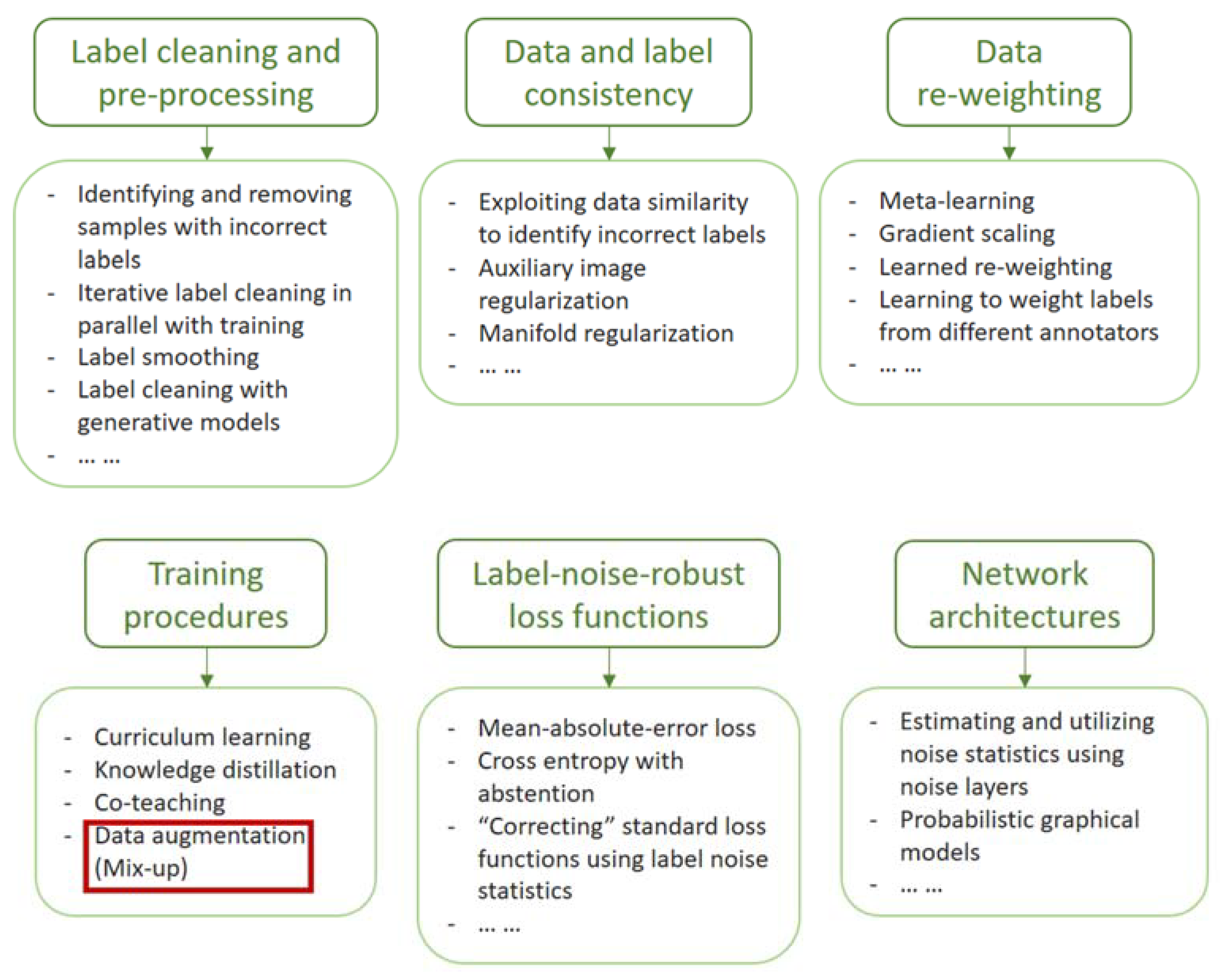
Figure 1. The overview of the state-of-the-art techniques of handling label noise in deep-learning-based approaches. The content was summarized based on Karimi et al. [39]. In this research, we chose “Data augmentation” by intermixing multi-source data to test whether the OBIA labels have potential to replace the Manual labels. The designation of experiments can be found in Section 2.5.
Applsci 12 11226 g001
Figure 2. The location of Kule and Nguenyyiel refugee camps together with their typical roof ontology of built-up structures. The subfigure (a) is the photo provided by MSF to reveal ground situations. The satellite imagery in the middle was retrieved from the wet season (22 June 2018), while (b,c) were retrieved from the dry season (24 March 2017). Yellow boundary: an example showing residents putting a brown cloth on the top of refugee tents. Red boundary: an example showing the dwelling roof turned from bright-colored to brownish due to rusting and/or sand. Green boundary: examples of three types of built-up structures. Blue boundary: an example showing trees can occlude built-up structures in satellite imagery.
Applsci 12 11226 g002
Figure 3. The examples of the OBIA labels and the Manual labels of built-up structures in the Kule and Nguenyyiel refugee camps during the dry and the wet seasons.
Applsci 12 11226 g003
Figure 4. The brief process of data preparation.
Applsci 12 11226 g004
Figure 5. The general structure of ResNet34-UNet.
Applsci 12 11226 g005
Figure 6. The basic structure of Encoder 1 and Decoder 4 of the ResNet34-UNet.
Applsci 12 11226 g006
Figure 7. The designation of experiments for Scenario I and Scenario II. KuleDry means data from the Kule refugee camp during the dry season. AccKD means the accuracy of the model tested by data from KuleDry. Ngu denotes the Nguenyyiel refugee camp. Other abbreviations in Scenario I follow analogous rules. The FT in Scenario II denotes fine-tuning.
Applsci 12 11226 g007
Figure 8. The spatial distribution of predicted FP (blue) and FN (red) pixels of the OBIA-OCOS model (a) and the Manual-OCOS model (b) from the Kule Wet case.
Applsci 12 11226 g008
Figure 9. (1) The annotated errors in the original OBIA labels and (2) examples (AE) showing the differences in FP (blue) and FN (red) pixels between the OBIA-OCOS model (middle) and the Manual-OCOS model (right) from the Kule Wet case.
Applsci 12 11226 g009
Table 1. The number of training and validation patches for the OBIA labels and Manual labels.
Refugee CampSeasonTrainingValidation
OBIAManualOBIAManual
KuleDry82538286917921
Wet79308109881901
NguenyyielDry68066745756749
Wet81068145901905
Table 2. The IoU values of built-up structures of all implemented experiments (OCOS: One Camp One Season; OCTS: One Camp Two Seasons; TCOS: Two Camps One Season; TCTS: Two Camps Two Seasons). The mean IoU values can be found in Table A2 in Appendix A.
Refugee CampSeasonTraining StrategyBaselineScenario IScenario II
ManualOBIA10%20%30%40%50%
KuleDryOCOS0.58570.51130.58290.60330.60190.59690.5999
OCTS0.58280.52020.58360.59270.59360.59580.5917
TCOS0.58870.52770.59160.59270.59270.59340.5927
TCTS0.58840.52760.56960.58470.58360.58660.5830
KuleWetOCOS0.64000.55390.63860.65410.65690.64120.6425
OCTS0.64590.54340.61880.63890.64460.63250.6413
TCOS0.63870.52730.64150.64700.64800.64930.6451
TCTS0.63390.55730.62960.63270.64800.64040.6364
NguenyyielDryOCOS0.63770.60510.63590.63930.63940.63890.6353
OCTS0.63880.60740.61290.63020.63750.63690.6366
TCOS0.63790.60510.63330.63710.63800.63850.6375
TCTS0.63910.61070.63990.64930.64710.64810.6440
NguenyyielWetOCOS0.64720.61960.64910.65380.65220.64930.6477
OCTS0.64650.61680.64860.65170.65180.64800.6452
TCOS0.65070.61670.66080.66360.66300.66110.6653
TCTS0.66340.63020.63300.61520.66240.63530.6604
Table 3. The Recall values of built-up structures of all implemented experiments.
Refugee CampSeasonTraining StrategyBaselineScenario IScenario II
ManualOBIA10%20%30%40%50%
KuleDryOCOS0.68400.59120.73700.73130.73350.72990.7377
OCTS0.69100.57900.67980.70660.70710.71800.7135
TCOS0.69400.58790.70020.70350.70760.71350.7180
TCTS0.69590.59500.65530.69120.69220.70070.6960
KuleWetOCOS0.71160.61620.74700.75510.73240.73240.7349
OCTS0.72450.60050.67660.71200.72250.72280.7298
TCOS0.71480.57550.72090.72430.73070.74220.7377
TCTS0.71240.62340.69660.70510.73380.72810.7249
NguenyyielDryOCOS0.77600.70930.75360.76280.76230.76680.7679
OCTS0.76570.71100.74930.75520.76830.76350.7651
TCOS0.76980.70430.78630.76590.76670.76880.7677
TCTS0.77130.71860.75620.77790.77820.78250.7784
NguenyyielWetOCOS0.75530.70420.74740.75950.76940.76280.7553
OCTS0.76080.70450.74870.75920.76210.75950.7552
TCOS0.76380.68900.76270.77120.77170.77240.7747
TCTS0.77120.71380.72450.76260.77540.76670.7703
Table 4. The Precision values of built-up structures of all implemented experiments.
Refugee CampSeasonTraining StrategyBaselineScenario IScenario II
ManualOBIA10%20%30%40%50%
KuleDryOCOS0.79090.80290.73600.77520.77040.76610.7625
OCTS0.78820.83670.80470.78620.78710.77770.7760
TCOS0.79500.83740.79230.79010.78490.77910.7726
TCTS0.79210.82320.81320.79140.78820.78270.7822
KuleWetOCOS0.86420.84550.84020.83460.83740.83740.8364
OCTS0.85620.85110.87870.86160.85680.83520.8410
TCOS0.85730.86290.85350.85830.85120.83850.8372
TCTS0.85180.84020.86740.86030.84710.84180.8389
NguenyyielDryOCOS0.78150.80480.80280.79790.79870.79300.7863
OCTS0.79400.80660.77100.79210.78910.79340.7912
TCOS0.78830.81110.76500.79110.79180.79020.7899
TCTS0.78860.80260.80630.79710.79350.79050.7886
NguenyyielWetOCOS0.81890.83760.83160.82450.81060.81350.8198
OCTS0.81140.83200.82910.82150.81830.81540.8159
TCOS0.81470.85450.83180.82630.82470.82100.8249
TCTS0.82600.84320.83370.76100.81960.78760.8224
Publisher’s Note: MDPI stays neutral with regard to jurisdictional claims in published maps and institutional affiliations.