Article

A Soybean Classification Method Based on Data Balance and Deep Learning

School of Mechanical Engineering, Xijing University, Xi’an 710123, China
*
Authors to whom correspondence should be addressed.
Appl. Sci. 2023, 13(11), 6425; https://doi.org/10.3390/app13116425
Submission received: 1 April 2023 / Revised: 15 May 2023 / Accepted: 22 May 2023 / Published: 24 May 2023
(This article belongs to the Special Issue Advanced Machine Learning and Scene Understanding in Images and Data)

Abstract

:
Soybean is a type of food crop with economic benefits. Whether they are damaged or not directly affects the survival and nutritional value of soybean plants. In machine learning, unbalanced data represent a major factor affecting machine learning efficiency, and unbalanced data refer to a category in which the number of samples in one category is much larger than that in the other, which biases the classification results towards a category with a large number of samples and thus affects the classification accuracy. Therefore, the effectiveness of the data-balancing method based on a convolutional neural network is investigated in this paper, and two balancing methods are used to expand the data set using the over-sampling method and using the loss function with assignable class weights. At the same time, to verify the effectiveness of the data-balancing method, four networks are introduced for control experiments. The experimental results show that the new loss function can effectively improve the classification accuracy and learning ability, and the classification accuracy of the DenseNet network can reach 98.48%, but the classification accuracy will be greatly reduced by using the data-augmentation method. With the binary classification method and the use of data-augmentation data sets, the excessive number of convolution layers will lead to a reduction in the classification accuracy and a small number of convolution layers can be used for classification purposes. It is verified that a neural network using a small convolution layer can improve the classification accuracy by 1.52% using the data-augmentation data-balancing method.

1. Introduction

Soybean is an annual herb and is the most important legume in the world. Soybean is rich in nutrients such as oil and protein, which have been widely used in the medical and food fields [1]. In daily consumption and soybean planting, the damage degree of soybean directly affects the nutritional value and survival rate of the plant. Therefore, it is very important to distinguish damaged soybeans from non-damaged soybeans. According to the Chinese national soybean quality grading standard, soybean quality grading uses parameters such as the integrity, damage rate, color, and odor of the soybeans [2].
Machine vision can capture an image of the target, and through the computer, can extract the pixel distribution, brightness, and color of the image and other information that can discriminate the measured target. Compared with traditional manual detection, machine vision detection technology has been widely used in grain appearance quality detection due to its high subjectivity and speed, allowing rapid and indirect contact with the measured target to complete the detection purpose [3].
Wu Gang designed a machine-vision-based corn-ear detection method, binarized the images, and then identified them by extracting local grain features with high accuracy [4]. Xie Weijun et al., used the color difference of different regions of carrots, determined the threshold of different regions using statistical methods in HSV color space, and then achieved the surface defect recognition of carrots by comparing the shape difference of normal carrots and defective carrots [5]. Wang Qiaohua et al., combined machine vision and near-infrared spectroscopy to extract the color feature values of the images to classify preserved eggs into edible eggs and inedible eggs, and then obtained the spectra of the two preserved eggs by near-infrared spectroscopy and realized the classification of preserved eggs using a competitive adaptive reweighting algorithm [6]. Lin Ping et al., proposed a soybean quality discrimination method based on the visible spectral map. By extracting the multi-scale spatial gradient and chromatic aberration components of the soybean visible spectrum, a visual dictionary is formed by the Kernel-means clustering algorithm, and then the multi-modal dictionary features are used for classification; its recognition accuracy can reach 92.7% [7].
With the development of deep learning and convolutional neural networks, the traditional machine vision recognition system has also changed. Through the combination of deep-learning and machine-vision technology, the classification effect can be improved automatically by automatic learning [8], so machine vision technology has been more widely used [9]. In quality classification in agriculture, grain and cash crops such as pistachio [10], jujube [11], and hazelnut [12] can be detected. There are also important applications in seed classification and identification. Xie Weijun et al., recognized Camellia oleifera seeds according to convoluted neural networks [13], and Gulzar Yonis proposed an algorithm that can recognize multiple types of seeds and has high accuracy [14].
At the same time, convolution neural networks can also be widely used in medicine to help solve problems. Nasim Sirjani and others developed an improved version of the InceptionV3 network, which originally classified breast lesions and had high recognition accuracy [15]. Zehra Karapinar Senturk proposed a deep-learning-based method to identify arrhythmia (ARR), congestive heart failure (CHF), and normal sinus rhythm (NSR) for cardiovascular diseases (CVD), and the recognition accuracy reached 98.7% [16]. Abhishek Agnihotri used machine learning methods to evaluate and identify COVID-19, putting forward the future development prospect of machine learning applied to medicine [17].
In agricultural detection, element deficiency disease identification of soybean leaves can be detected by deep-learning methods and training through pictures collected by machine vision [18], and it can also be applied to other agricultural pests and diseases [19]. Laura Gómez-Zamanillo and others put forward a damage-assessment method, which can identify crops and weeds in the greenhouse with high accuracy [20]. In industry, it is mainly used to detect surface defects of workpieces, and through machine vision technology, it can identify small defects on the surface of workpieces [21] and diagnose faults in rotating parts [22].
The classification technique based on deep learning can improve the accuracy of classification in theory, but the data balance of different types of data sets will affect the performance of the network and make the network training effect unstable [23]. Traditional classification methods assume that the data is balanced. However, when the number of classes is uneven, the classification model tends to be biased towards the larger number of classes, which leads to a decrease in the recognition accuracy for the smaller number of classes [24]. To verify the effect of data balance and network structure on the accuracy of soybean integrity recognition, AlexNet, VGG, ResNet, and DenseNet networks were used to carry out the experiments in this paper to achieve the classification requirements of qualified soybeans. The classification accuracy was improved by data augmentation and referencing different loss functions, and the data were balanced to obtain a better classification effect.

2. Material and Data Collection

2.1. Vision System and Image Acquisition

Soybean was selected as the research object in this study. The acquisition equipment was a Viscan MV-HP505GM/C industrial camera with a resolution of 2595 × 1944, a manual zoom 5-megapixel lens. Other equipment included a support, computer, and light source. The software system was mainly based on OpenCV and the Torch function library, with Python as a programming language. The camera was connected to the computer to acquire images. The image acquisition system is shown in Figure 1.
In the practical application of soybean detection, the number of defective soybeans is often relatively small, while the number of intact soybeans is relatively large. To better simulate the actual situation and improve the generality of the network, an unbalanced soybean data set was used.
The image-classification algorithm used in this paper took soybeans as the research object and divided the soybeans into two categories according to the integrity of soybean standards: intact soybeans and damaged soybeans. Figure 2 shows pictures of the two types of soybeans: (a) intact soybean, with a round and smooth appearance, and (b) (c) (d) damaged soybean, defective soybean, and worm-eaten soybean, all of which were unqualified soybeans.

2.2. Image Preprocessing

To obtain a single soybean image, the original collected image needs to be processed. In OpenCV, the collected images were converted into gray maps, and the contour curves of soybean were obtained by binarization processing and contour detection after opening and closing the images, and the image background was removed by an operation to obtain a better training effect, the above processing procedure is shown in Figure 3. Finally, the area of the contour region was calculated, the minimum external rectangle of the soybean was drawn, and the image was cropped to obtain a single soybean image.

2.3. Data-Augmentation Processing

Data augmentation is a widely known strategy for effectiveness improvement in computer vision models such as deep convolutional neural networks [25]. In the data set, the number of intact soybean images was 393, the number of damaged soybean images was 92, and the ratio of the two types of images was 1:8.5; therefore, there was a data imbalance. The preprocessed data set was enhanced; the training data was rotated, flipped, and scaled; and the training data samples were reasonably adjusted by adding salt and data enhancement methods such as per-noise and Gaussian noise, and by improving brightness. The numbers of two the types of sample enhanced by data were 787 and 829, respectively, and the difference between the two types of samples was within 5%, so it was judged that the data set tended to be balanced (Table 1).

2.4. Focal-Loss Function and Label-Smoothing

The focal-loss function has been shown to have the characteristics of mining difficult samples and adjusting sample imbalance problems [26]. Because there was a big gap between qualified soybean images and unqualified soybean images in this experimental data set, it would affect the accuracy of classification judgment in network training. The focal-loss function was used to allocate the weights of two samples to balance the data. At the same time, to slow down the over-fitting degree of the network and improve the recognition accuracy, it was proposed to introduce label-smoothing into the classification network. By creating a new loss function on the basic network model, the focal-loss function allocates two sample weight functions, and the label-smoothing function is realized at the same time.

2.4.1. Focal-Loss Function Principle

Cross-entropy loss is a type of loss function that is often used in network training. In the face of unbalanced data sets, it has a relatively low recognition degree with a few samples. “Focal loss is a cross-entropy loss of dynamic scaling. By inserting a dynamic scaling factor, the weight of both challenging and easy samples can be adjusted in the training process, thus biasing the center of gravity towards the more challenging samples.” [27]. The method is as follows:
Cross-entropy loss: Cross-entropy loss is based on a binary classification, which takes the following form:
CE p , y = log p if   y = 1 log 1 p otherwise .
where y takes values of 1 and −1 to represent the foreground and background, respectively. The value of p ranges from 0 to 1, which is the probability that the model predicts belonging to the foreground.
Defining a function about p:
p t = p if   y = 1 1 p otherwise .
Combined with the above formula, there is the following formula.
CE p , y = CE p t = log p t
Balanced cross entropy: Common solutions to class imbalance. A weight factor α ∈ [0, 1] is introduced, which is α when it is a positive sample and 1 − α when it is a negative sample. Therefore, the loss function formula is as follows:
CE p t = α t log p t
Focal loss: Although the balanced cross entropy solves the problem of positive and negative samples, the difficulty in distinguishing samples will still have an impact on network training, so a modulation factor is introduced to focus on the difficult samples, and the formula is as follows:
F L p t = 1 p t γ l o g p t
As a parameter, γ is in the range of [0, 5]. When γ becomes 0, it becomes the initial cross-entropy function.

2.4.2. Label-Smoothing Principle

As a parameter, γ ranges from [0, 5]. When γ becomes 0, it becomes the initial cross-entropy-loss function. Label-smoothing, also called label smooth regularization (LSR), refers to a regular update of the binary label vector y of the sample:
y = 1 ε y + ε / n
where ε is a small hyperparameter and n is the number of categories of classification (the number of bits of the label vector). y k is defined as the binary label vector value of the K-th category, the target is the real label value of the current category, and the I-th bit value of the one-hot code of the label vector is I, then there is
y k = 1 ε + ε / n i = t a r g e t ε / n i t a r g e t
Let α = ε + ε / n , then there is
y k = 1 α i = t a r g e t α / n 1 i t a r g e t
To sum up, we can establish that the focal-loss function of a single sample is defined as
L O S S = 1 n k = 1 n y k × 1 p t γ × l o g p t
At this time, the binary vector value y k i t a r g e t at the wrong label is no longer 0, so the process of minimizing L by Formula (9) of the loss function will no longer make the model learn in the direction that the difference between the correct prediction and the wrong label logits increases infinitely, thus solving the problem of overconfidence of the network.

2.5. Convolutional Neural Networks

Table 2 shows four types of neural networks used in the experiment, and there are some differences in the structure of each network.

2.6. DenseNet Neural Network Model

In this paper, the DenseNet network model, which is mainly composed of DenseBlock and Transition layers, was used as the main training network (shown in Figure 4). In each DenseBlock, the feature map size of each layer is consistent, and BN + ReLU + 1 × 1 Conv + BN + ReLU + 3 × 3 Conv is used as a nonlinear combination function for operation, in which the included 1 × 1 convolution can reduce the operation parameters and improve the operation efficiency. The transition layer connects two adjacent DenseBlocks to reduce the size of the feature map and compress the model. The transition layer consists of has the structure BN + ReLU + 1 × 1 Conv + 2 × 2 AvgPooling. For data sets entered into the DenseNet network, the input picture size was set to 224 × 224 and training was started after passing through a 7 × 7 convolution layer with a step size of 2, followed by a 3 × 3 MaxPooling layer with a step size of 2.

3. Results and Discussion

3.1. Experimental Data

The neural network selects AlexNet, VGG19, ResNet101, and DenseNet 121 networks to train the model. The data sets were randomly divided into training and test sets in a 70:30 ratio. The training set is used to train and control the model, while the test set is used to test the accuracy of the classification model.
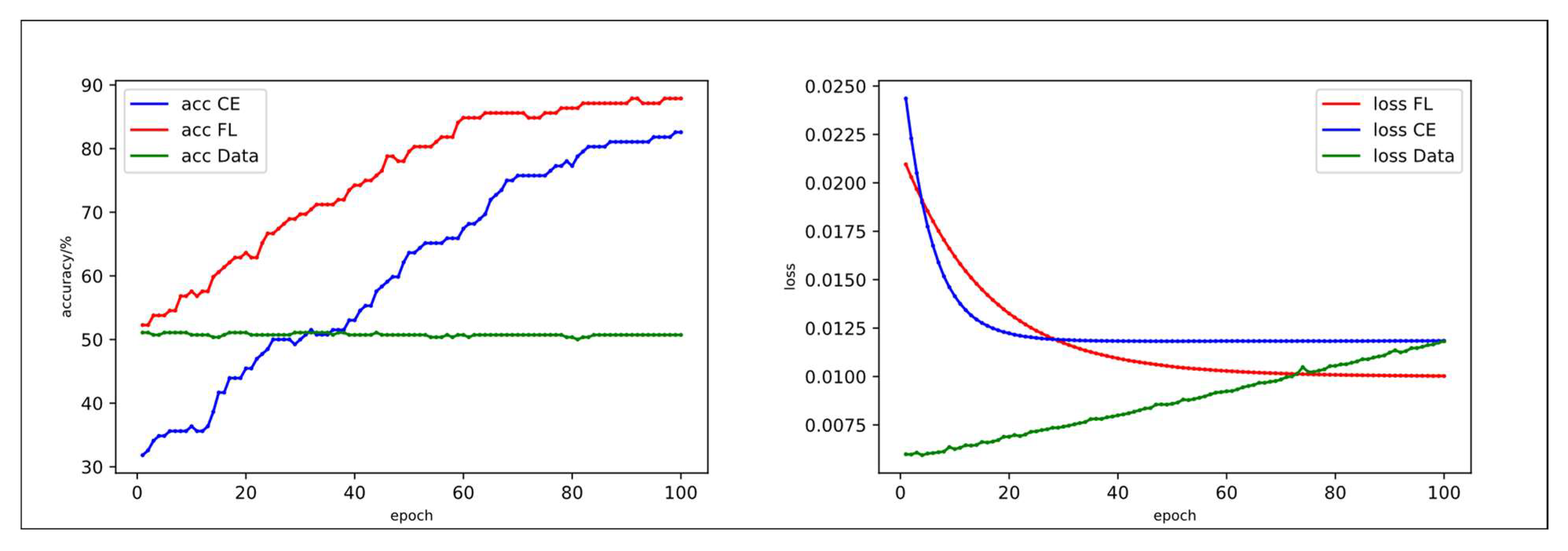
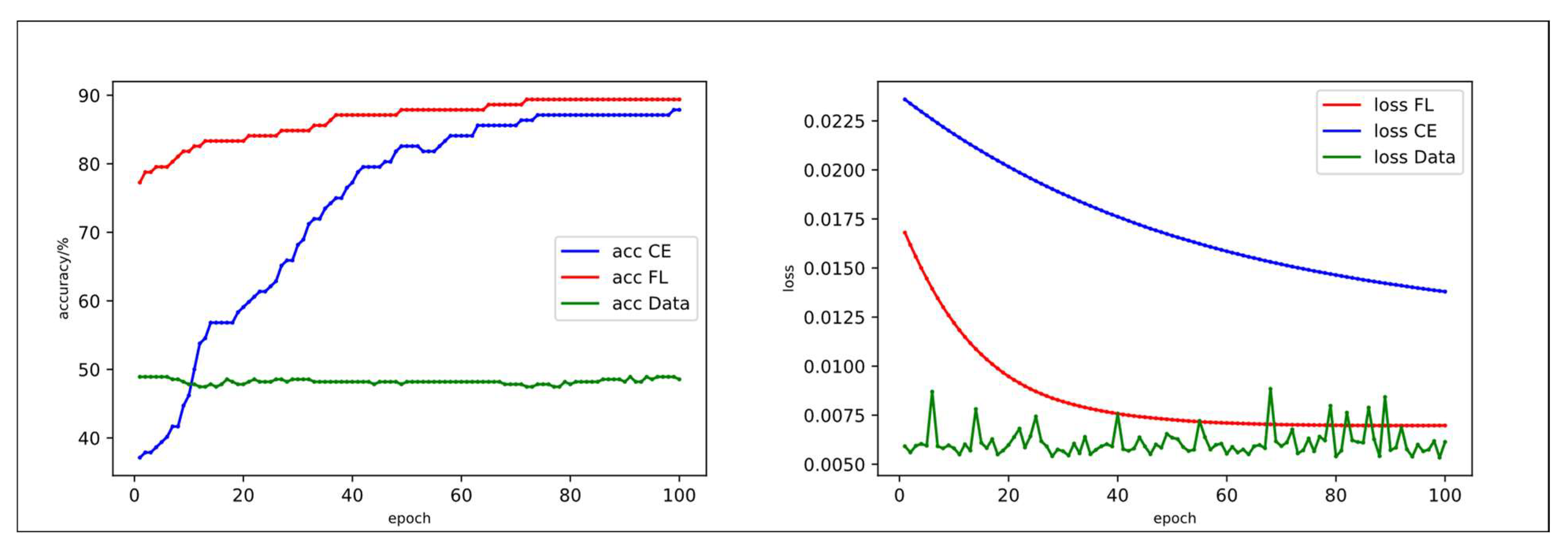
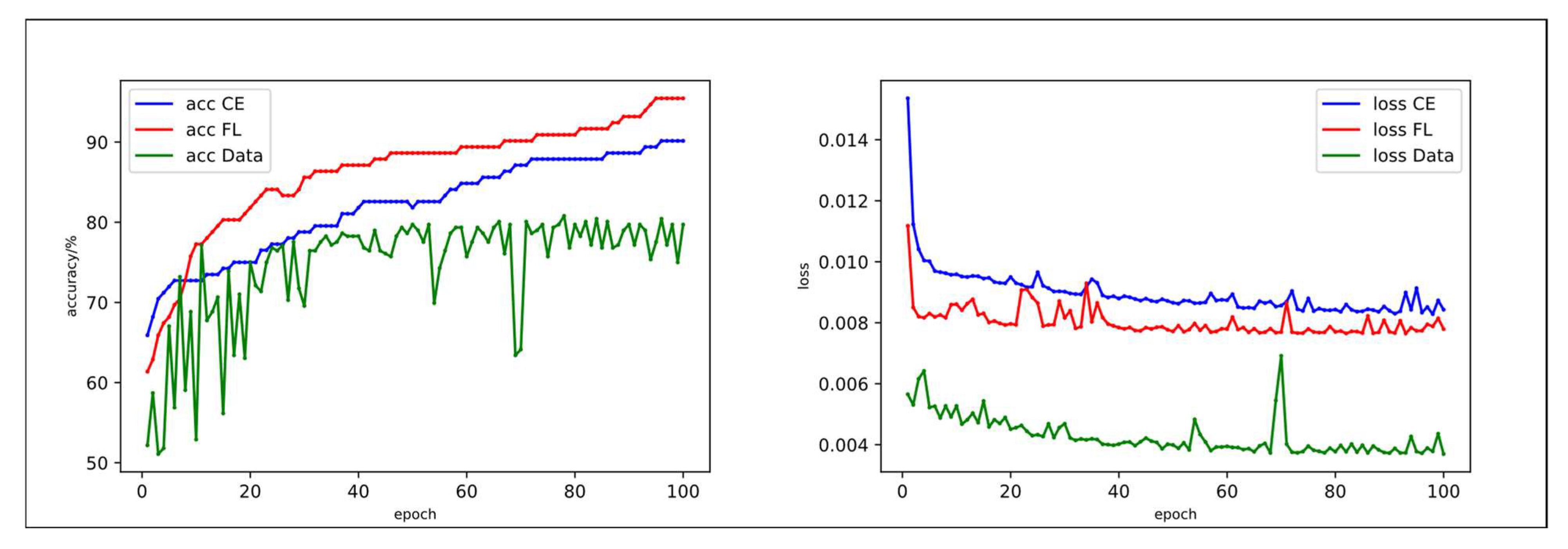
The following figure shows the changes in classification accuracy curves of different networks for different data sets. The abscissa epoch value is the training time, and the vertical coordinate accuracy and loss values are the values of the classification accuracy and loss function, respectively. When the accuracy value is higher, the accuracy value is higher, and the loss value is lower; this shows that the classifier works better in the relationship between the input data and output target, which is abbreviated as acc accuracy. CE in the figure represents the cross-entropy-loss function cross-entropy loss, FL is the loss function focal loss introduced in this paper for data imbalance, data represents the classification accuracy of network training using data-augmentation data sets.
Figure 5 and Figure 6 show the training situation of the AlexNet network and VGG network. In the training process of this network, selecting a larger learning rate will result in the overfitting of the network and lead to a decrease in the classification accuracy. Therefore, in the experiment, the learning rates of 0.000001 and 0.000003 were selected for the two networks, respectively. These could achieve higher classification progress without the overfitting phenomenon. In addition, it can be observed from the data curve in the figure that the introduction of the focal-loss function could effectively improve the classification accuracy. However, the data set using the data-augmentation method did not have the expected effect but caused a substantial decrease in classification accuracy.
Figure 7 and Figure 8 show the line graphs of the ResNet network and DenseNet network training. It can be observed from the data in the figure that the classification accuracy was be improved by using the focal-loss function. Because there were few samples in this experiment, the accuracy of classification was not much improved compared with the cross-entropy-loss function, and regarding the AlexNet network and VGG network, the use of data-augmentation data set training also decreased the classification progress, but its decrease was smaller than the AlexNet network and VGG network.
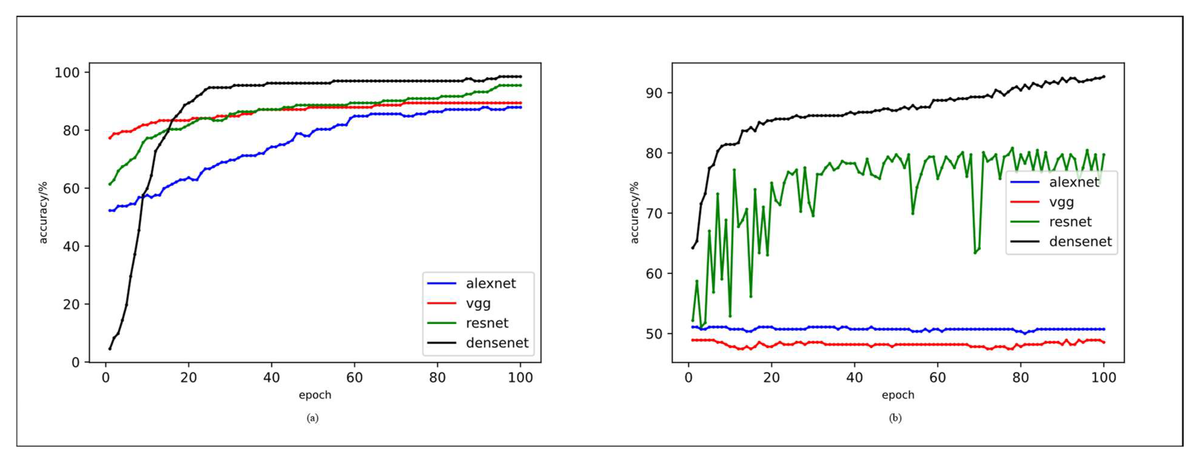
Figure 9 reflects the comparison of the classification accuracy of four networks in three cases, and it can be observed that the DenseNet network could achieve high classification accuracy in three cases.
Table 3 documents that the four networks tend to level out classification accuracy at loss values. The testing classification accuracy of the four networks was 89.20% when the cross-entropy-loss function was used, and 92.80% when focal loss was used as the loss function, indicating that the use of the focal-loss function could divide the data set sample weight and reduce the classification accuracy decline caused by data imbalance. However, after training the networks with the data-augmentation data set, the testing classification accuracy of all four networks decreased, and the average value decreased to 69.17%. Among them, the AlexNet network and VGG network received the most impact, followed by the ResNet network, and the DenseNet network received the least impact. For the four types of network in this experiment, two methods of data-balance processing could effectively reduce the loss value, and strengthen the learning ability of the network, so that the network could learn more content. The data-balance method was proven to be effective.

3.2. Data Analysis

Among the four networks in this experiment, the reason why VGG19 and AlexNet networks could not improve the classification accuracy in the face of training using data-augmentation data sets lay in their excessive convolution layers. In the experiment on soybean binary classification, due to the principle of the convolution neural network (Figure 10), too many convolution layers will make the noise in the image participate in the convolution training as image characteristics, so the final classification accuracy cannot achieve the expected effect.
Through the above experiments, it can be seen that too many convolution layers will reduce the classification accuracy, whereas a few convolution layers can achieve better classification results. To demonstrate this view, a low convolution layer neural network, Simple (Figure 11), with four convolution layers, two pooling layers, and two fully connected layers was reconstructed. The network structure extracted image features through the convolution layer, reduced parameters through the pooling layer, and reduced the number of channels from 512 to 256 compared with VGG neural network model. Finally, images were classified and recognized through two fully connected layers.
Figure 12 shows the convolutional network classification accuracy training, using a learning rate of 0.000002 in the training, training 100 times. The accuracy of classification training could reach 90.2% with data-augmentation data set training, 90.9% with the focal-loss function, and 88.6% with the cross-entropy-loss function. The experiment showed that the neural network with a low convolution layer could improve the classification accuracy by using the data-augmentation data set processing method and the focal-loss function in the soybean binary classification experiment.
In addition, the classification accuracy of ResNet and DenseNet networks was less affected by the data-augmentation data set. According to the experiments, the low convolution layer could achieve the desired effect; it was shown that when the soybean binary classification method used the data-augmentation data set, it was necessary to retain certain original image feature data to make the network have less impact on the sampled data set. The ResNet network uses the special structure of residual blocks (shown in Figure 13), x is the input value, and F(x) + x is the output value of this layer, which can combine the original data with the data processed by the hidden layer as the data of this layer. Thus, the residual blocks can retain the original input data and reduce the impact due to noise. Therefore, using the structure of residual blocks can protect the original features of the image, so ResNet is less affected by the data-augmentation data set and still maintains a high classification accuracy.
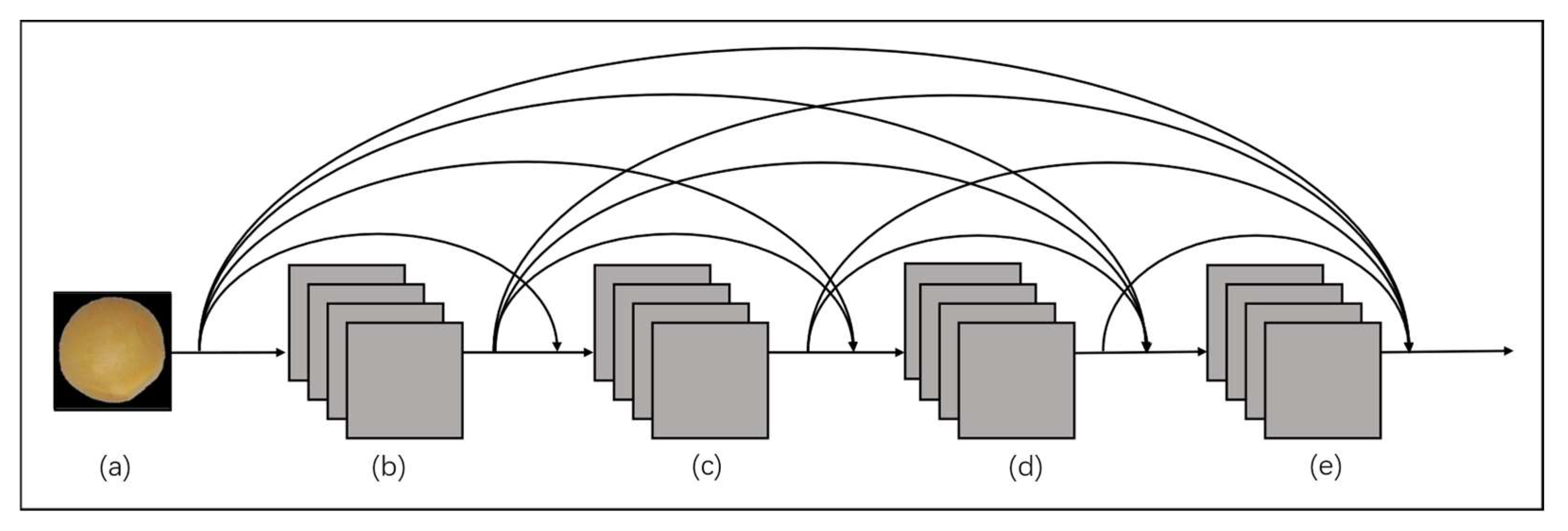
DenseBlock is a special structure in the DenseNet network. In DenseBlock, the current layer and all subsequent layers are closely connected, at which time the output of layer l can be x l = H l x 0 , x 1 , x l 1 . The partial structure of the DenseNet network is shown in Figure 14, where the input image data are x 0 and the data processed by the current layer (b) are xb, then the output data of this partial network are y = x 1 + x b + x c + x d + x e . Therefore, the DenseNet network can better save the input data and the original features of the image, avoiding too much noise due to too many convolution layers as image features to participate in soybean classification.
Three network structures, VGG19, Simple, and DenseNet, were selected for confusion verification, and over-sampled data sets were used for network training. Figure 15 shows the results of obfuscation verification. Among them, vgg19 (Figure 15a) had obvious shortcomings in identifying damaged soybeans; a neural network with low convolution levels and a DenseNet network could complete the classification well. In the face of binary classification, the neural network structure with low convolution levels and a DenseNet Block structure could achieve a better classification effect than the network with multiple convolution levels.

3.3. Data Analysis and Demonstration

From the above experimental results, it can be concluded that too many convolution layers will lead to a decline in classification accuracy when facing the binary classification problem, and the training data are oversampled. The problem of the decline of classification accuracy can be solved by reducing the convolution layers and transferring parameters between different convolution layers. To demonstrate the experimental conclusion, this paper used an open-source rice image data set, and selected two types of rice image data in the data set, Arborio, and Basmati, as training data to demonstrate the experimental conclusion. After the same data-augmentation method, there were 249 and 243 Arborio and Basmati rice image, respectively (Table 4).
Figure 16 shows the classification iteration of training VGG19, Simple, and DenseNet networks using oversampled data sets. From this image, it can be seen that using over-sampled data sets to train the network will lead to low classification accuracy, and will cause great changes to the classification accuracy of vgg19. However, at the lower level, the convolutional neural network and DenseNet network models are less affected. This is consistent with the experimental conclusion obtained from the soybean classification experiment. Therefore, data-augmentation of the data set in binary classification will lead to a decline in the classification accuracy of neural networks with more convolution layers such as AlexNet and VGG but has less influence on low-level convolution neural networks and neural networks with a residual block and DenseNet Block structure.

4. Conclusions

The data-balance method that references focal loss as a loss function can effectively improve the detection accuracy of the network. The classification accuracy of the four networks was improved by 3.60%, and the loss value also decreased, which proves that the focal-loss function can achieve the expected results. In addition, in this experiment, all four networks had high classification accuracy, but the optimized DenseNet network had the highest test accuracy, at 98.48%, and it can be used as the primary choice for soybean appearance quality detection.
In the face of training with data-augmentation data sets in soybean binary classification experiments, VGG and AlexNet multi-convolution network structures cannot effectively convolute soybean species, because multi-layer convolution introduces non-classified features into convolution calculation causing a decrease in accuracy, and it is experimentally proved that a small number of convolution layers can be used to prevent non-image features from participating in convolution and protect the original image features when processing simple image classification. DenseNet and ResNet networks face the data-augmentation data set because residual blocks can effectively transmit information and protect the original characteristics of the image, the classification accuracy is less affected, and they will not have a serious impact on the overall accuracy of the network.
In this paper, the loss function of the DenseNet121 network was modified so that it could more effectively deal with the problem of data imbalance. Through experiments, the impression of the over-sampled image-enhancement method on neural networks was verified, which has potential in the face of image noise.

Author Contributions

Conceptualization, N.Z., E.Z. and F.L.; methodology and formal analysis, E.Z.; investigation, F.L.; writing—original draft preparation, E.Z.; writing and review N.Z., E.Z. and F.L. All authors have read and agreed to the published version of the manuscript.

Funding

This work was supported by Xijing University and National Science and Technology Major Project.

Institutional Review Board Statement

Not applicable.

Informed Consent Statement

Not applicable.

Data Availability Statement

The data that support the findings of this study are available from the corresponding author upon reasonable request.

Conflicts of Interest

The authors declare no conflict of interest.

References

  1. Li, Y. Progress in Soybean Processing. Soybean Sci. Technol. 2022, 176, 14–26. [Google Scholar]
  2. Chen, P.; Hua, L.; Wang, W.; Bao, H.; Wang, D.; Chen, J.; Huang, T. Correlation analysis between the internal quality of imported soybeans and their appearance quality traits. Chin. Oil 2011, 36, 30–32. [Google Scholar]
  3. Chen, W.; Li, W.; Li, Z. Progress in Machine Vision Based Quality Testing of Grain Appearance. J. Henan Univ. Technol. (Nat. Sci. Ed.) 2022, 43, 118–128. [Google Scholar]
  4. Wu, G.; Wu, Y.; Chen, D.; Li, B.; Zhen, Y. Measurement of ear trait parameters of maize based on machine vision. J. Agric. Mach. 2020, 51, 357–365. [Google Scholar]
  5. Xie, W.; Wei, S.; Wang, F.; Yang, G.Z.; Ding, X.; Yang, D. Identification of Carrot Surface Defects Based on Machine Vision. J. Agric. Mach. 2020, 51, 450–456. [Google Scholar]
  6. Wang, Q.; Mei, L.; Ma, M.; Gao, S.; Li, Q. Non-destructive detection and grading of preserved eggs using machine vision and near-infrared spectroscopy. J. Agric. Eng. 2019, 35, 314–321. [Google Scholar]
  7. Lin, P.; He, J.; Zou, Z.; Chen, Y. Discriminant method of soybean appearance quality based on the visible spectrum. J. Opt. 2019, 39, 208–215. [Google Scholar]
  8. Yang, B.; Zhong, J. Review of research progress of convolutional neural networks. J. Univ. South China (Nat. Sci. Ed.) 2016, 30, 66–72. [Google Scholar]
  9. Chen, C.; Qi, F. Development of Convolutional Neural Networks and Their Applications in the Field of Computer Vision. Comput. Sci. 2019, 46, 63–73. [Google Scholar]
  10. Gao, Q.; Ni, J.; Yang, H.; Han, Z. The visual detection method of pistachio fruit quality based on data balance and deep learning. J. Agric. Mach. 2021, 52, 367–372. [Google Scholar]
  11. Guo, Z.; Zheng, H.; Xu, X.; Ju, J.; Zheng, Z.; You, C.; Gu, Y. Quality grading of jujubes using composite convolutional neural networks in combination with RGB color space segmentation and deep convolutional generative adversarial networks. J. Food Process Eng. 2020, 44, e13620. [Google Scholar]
  12. Ünal, Z.; Aktaş, H. Classification of hazelnut kernels with deep learning. Postharvest Biol. Technol. 2023, 197, 112225. [Google Scholar] [CrossRef]
  13. Xie, W.; Ding, Y.; Wang, F.; Wei, S.; Yang, D. Integrity Identification of Camellia oleifera Seeds Based on Convolutional Neural Network. J. Agric. Mach. 2020, 51, 13–21. [Google Scholar]
  14. Gulzar, Y.; Hamid, Y.; Soomro, A.B.; Alwan, A.A.; Journaux, L. A Convolution Neural Network-Based Seed Classification System. Symmetry 2020, 12, 2018. [Google Scholar] [CrossRef]
  15. Sirjani, N.; Oghli, M.G.; Tarzamni, M.K.; Gity, M.; Shabanzadeh, A.; Ghaderi, P.; Shiri, I.; Akhavan, A.; Faraji, M.; Taghipour, M. A novel deep learning model for breast lesion classification using ultrasound Images: A multicenter data evaluation. Phys. Med. 2023, 107, 102560. [Google Scholar] [CrossRef] [PubMed]
  16. Senturk, Z.K. From signal to image: An effective preprocessing to enable deep learning-based classification of ECG. Mater. Today Proc. 2022, 81, 1–9. [Google Scholar]
  17. Agnihotri, A.; Kohli, N. Challenges, opportunities, and advances related to COVID-19 classification based on deep learning. Data Sci. Manag. 2023, 6, 98–109. [Google Scholar] [CrossRef]
  18. Xiong, J.; Dai, S.; Chu, J.; Lin, X.; Huang, Q.; Yang, Z. Deep learning-based detection method for leaf deficiency symptoms in soybean growing period. J. Agric. Mach. 2020, 51, 195–202. [Google Scholar]
  19. Guo, W.; Feng, Q.; Li, X. Research progress of convolutional neural network model based on crop disease detection and recognition. Chin. J. Agric. Mach. Chem. 2022, 43, 157–166. [Google Scholar]
  20. Gómez-Zamanillo, L.; Bereciartua-Pérez, A.; Picón, A.; Parra, L.; Oldenbuerger, M.; Navarra-Mestre, R.; Klukas, C.; Eggers, T.; Echazarra, J. Damage assessment of soybean and redroot amaranth plants in the greenhouse through biomass estimation and deep learning-based symptom classification. Smart Agric. Technol. 2023, 81, 100243. [Google Scholar] [CrossRef]
  21. Zheng, D.; Zhou, T.; Zeng, Z. Optical Component Defect Recognition Technology Applicable to Intelligent Industrial Monitoring. Lab. Res. Explor. 2022, 41, 13–17. [Google Scholar]
  22. Liu, L.; Li, S.; Lu, J. A Review of Fault Diagnosis of Rotary Drive Components Based on Convolutional Neural Networks. Mech. Des. 2022, 39, 1–8. [Google Scholar]
  23. Li, Y.; Chai, Y.; Hu, Y.; Yi, H. Summary of unbalanced data classification methods. Control. Decis. Mak. 2019, 34, 673–688. [Google Scholar]
  24. Chen, S.; Shen, S.; Li, D. Unbalanced Data Integration Learning Method Based on Sample Weight Updated. Comput. Sci. 2018, 45, 31–37. [Google Scholar]
  25. Dourado, C. Data Augmentation policies and heuristics effects over dataset imbalance for developing plant identification systems based on Deep Learning: A case study. Rev. Bras. De Comput. Apl. 2022, 14, 85–94. [Google Scholar] [CrossRef]
  26. Fu, B.; Tang, X.; Xiao, T. Research on Focal Loss Function Applied to Image Emotion Analysis. Comput. Eng. Appl. 2020, 56, 179–184. [Google Scholar]
  27. Lin, T.Y.; Goyal, P.; Girshick, R.; He, K.; Dollár, P. Focal Loss for Dense Object Detection. IEEE Trans. Pattern Anal. Mach. Intell. 2017, 99, 2999–3007. [Google Scholar]
  28. Krizhevsky, A.; Sutskever, I.; Geoffrey, E. Hinton. ImageNet classification with deep convolutional neural networks. Commun. ACM 2017, 60, 84–90. [Google Scholar] [CrossRef]
  29. Simonyan, K.; Zisserman, A. Very Deep Convolutional Networks for Large-Scale Image Recognition. arXiv 2014, arXiv:1409.1556. [Google Scholar]
  30. He, K.; Zhang, X.; Ren, S.; Sun, J. Deep Residual Learning for Image Recognition. In Proceedings of the IEEE Conference on Computer Vision and Pattern Recognition 2016, Las Vegas, NV, USA, 26 June–1 July 2016. [Google Scholar]
  31. Huang, G.; Liu, Z.; Van Der Maaten, L.; Weinberger, K.Q. Densely Connected Convolutional Networks. In Proceedings of the IEEE Conference on Computer Vision and Pattern Recognition 2017, Honolulu, HI, USA, 21–26 July 2017. [Google Scholar]
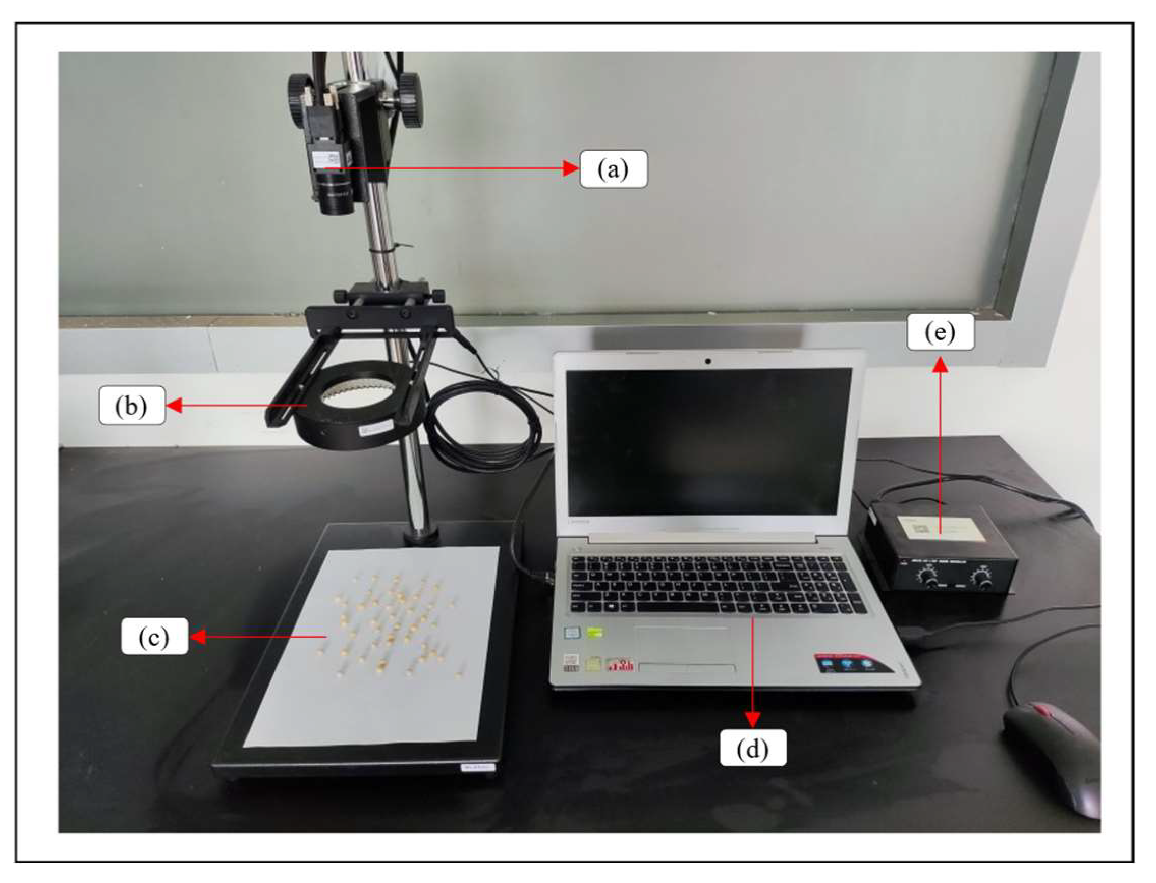
Figure 1. Image acquisition system: (a) CCD camera, (b) light source, (c) measured soybean, (d) computer, and (e) light-source adjusting mechanism.
Applsci 13 06425 g001
Figure 2. Soybean images: (a) intact soybean, (b) damaged soybean, (c) defective soybean, and (d) soybean eaten by insects.
Applsci 13 06425 g002
Figure 3. Image preprocessing of soybean. (a) Original image of soybeans, (b) gray image of soybeans, (c) outline image of soybeans, (d) circumscribed rectangles of soybeans, and (e) single soybean image.
Applsci 13 06425 g003
Figure 4. DenseNet network structure diagram.
Applsci 13 06425 g004
Figure 5. Curve variation and loss value diagram of AlexNet network training classification accuracy.
Applsci 13 06425 g005
Figure 6. Variation of training classification accuracy curve and loss value diagram of VGG network.
Applsci 13 06425 g006
Figure 7. Curve variation and loss value diagram of ResNet network training classification accuracy.
Applsci 13 06425 g007
Figure 8. Variation in training classification accuracy curve and loss value diagram of DenseNet network.
Applsci 13 06425 g008
Figure 9. Four types of network classification accuracy training situations; (a) original loss function training network; (b) oversampled data set training network.
Applsci 13 06425 g009
Figure 10. Schematic diagram of convolutional neural network.
Applsci 13 06425 g010
Figure 11. Schematic diagram of the Simple network structure.
Applsci 13 06425 g011
Figure 12. The curve of training accuracy of the convolutional network.
Applsci 13 06425 g012
Figure 13. Schematic diagram of the residual block.
Applsci 13 06425 g013
Figure 14. The internal structure of DenseBlock: (a) is an input image and (be) represent a BN and a convolution layer.
Applsci 13 06425 g014
Figure 15. Confusion matrix verification of three types of network models: (a) VGG19 model confusion verification result, (b) Simple network confusion verification result, and (c) DenseNet model confusion verification result.
Applsci 13 06425 g015
Figure 16. Iteration of classification accuracy of three networks using over-sampled rice data sets: (a) training result of the VGG19 network model, (b) training result of the Simple network model, and (c) training result of the DenseNet network model.
Applsci 13 06425 g016
Table 1. Number of samples in a dataset.
Data SetIntact Soybean SampleBroken Soybean Sample
Original data set43992
Data-augmentation data set787829
Table 2. Four types of networks were used in the experiment.
Convolutional Neural
Network
Characteristic
AlexNetAlexNet applied ReLU as the activation function of a convolutional neural network in CNN for the first time and proposed that the deeper network structure uses the stacked convolutional layer to extract image features, and uses Dropout and data enhancement data-augmentation to suppress overfitting [28].
VGGVGG realizes image recognition through the set convolution layer, pooling layer, and full connection layer, and the whole network uniformly uses the same size of convolution kernel size (3 × 3) and maximum pooling size (2 × 2), which can improve the performance by deepening the network [29].
ResNetResNet adds a direct channel to different convolution layers of the network to allow the original input information to be transmitted directly to the later layers. This approach greatly reduces the problem of gradient vanishing [30].
DenseNetDenseNet is a dense convolutional neural network with a deeper number, which connects all layers under the premise of ensuring the maximum information transmission between layers in the network. A 1 × 1 convolution kernel was also inserted to reduce the feature map and parameters [31].
Table 3. Experimental results of network training.
CNN ModelCE Loss FunctionFocal-Loss FunctionOversampling
Training Accuracy/%Test Accuracy/%Training Accuracy/%Test Accuracy/%Training Accuracy/%Test Accuracy/%
AlexNet85.9982.5888.6087.8756.3050.72
VGG89.9087.8789.5889.3952.2648.55
ResNet90.5590.1596.4195.4589.2779.71
DenseNet96.7496.2199.3598.4897.8397.71
Average value90.8089.2093.4992.8073.9269.17
Table 4. Number of samples in the rice dataset.
Data SetIntact Soybean SampleBroken Soybean Sample
Original data set249243
Oversampled data set700659
Disclaimer/Publisher’s Note: The statements, opinions and data contained in all publications are solely those of the individual author(s) and contributor(s) and not of MDPI and/or the editor(s). MDPI and/or the editor(s) disclaim responsibility for any injury to people or property resulting from any ideas, methods, instructions or products referred to in the content.