Abstract
In recent years, CO2 flooding has emerged as an efficient method for improving oil recovery. It also has the advantage of storing CO2 underground. As one of the promising types of CO2 enhanced oil recovery (CO2-EOR), CO2 water-alternating-gas injection (CO2-WAG) can suppress CO2 fingering and early breakthrough problems that occur during oil recovery by CO2 flooding. However, the evaluation of CO2-WAG is strongly dependent on the injection parameters, which in turn renders numerical simulations computationally expensive. So, in this work, machine learning is used to help predict how well CO2-WAG will work when different injection parameters are used. A total of 216 models were built by using CMG numerical simulation software to represent CO2-WAG development scenarios of various injection parameters where 70% of them were used as training sets and 30% as testing sets. A random forest regression algorithm was used to predict CO2-WAG performance in terms of oil production, CO2 storage amount, and CO2 storage efficiency. The CO2-WAG period, CO2 injection rate, and water–gas ratio were chosen as the three main characteristics of injection parameters. The prediction results showed that the predicted value of the test set was very close to the true value. The average absolute prediction deviations of cumulative oil production, CO2 storage amount, and CO2 storage efficiency were 1.10%, 3.04%, and 2.24%, respectively. Furthermore, it only takes about 10 s to predict the results of all 216 scenarios by using machine learning methods, while the CMG simulation method spends about 108 min. It demonstrated that the proposed machine-learning method can rapidly predict CO2-WAG performance with high accuracy and high computational efficiency under conditions of various injection parameters. This work gives more insights into the optimization of the injection parameters for CO2-EOR.
1. Introduction
With the continuous improvement of oil and gas exploration and development, the proportion of heterogeneous and low-permeability reservoirs in exploration and development is gradually increasing. Using conventional water injection to develop low-permeability reservoirs results in a low recovery factor [1]. Compared to water, CO2 is less viscous and can enter into small pores more easily, which can reduce the viscosity of crude oil, expand the volume of crude oil, improve the mobility ratio, and thus increase the oil recovery factor [2,3]. Therefore, CO2-enhanced oil recovery (CO2-EOR) has great potential for developing low-permeability reservoirs. In addition to this, CO2-EOR can sequestrate CO2 underground, which can help in achieving carbon neutrality [4]. However, in the CO2 flooding method, during gas injection, the low viscosity of CO2 may lead to a phenomenon referred to as viscous fingering. This results in an unfavorable mobility ratio, which seriously affects the improvement of swept volume [5]. Moreover, due to its low density, CO2 can easily escape to the upper part of the reservoir, forming a fugitive flow channel [6]. This also constitutes a drawback for CO2 flooding as it leads to a reduction of the swept volume.
In response to the problems of waterflooding and CO2 flooding, researchers proposed CO2-WAG methods [7]. This technology was first used by Mobil in 1957 in a sandstone reservoir in Alberta, Canada. It combines the characteristics of water flooding and CO2 flooding, which increases the macroscopic sweep efficiency and thus improves the overall oil displacement efficiency. In addition, CO2-WAG can mitigate the issue of rapid CO2 flow and increase the gas phase’s flow resistance. It can also lower the resistance to the flow of the water phase and increase the mobility ratio. As a result of this, recovery efficiency can be greatly improved [7]. It has been reported that 80% of oilfield projects in the US using WAG technology have achieved good results [8]. Skauge et al. [9] studied 59 WAG fields and found that the average recovery of crude oil was improved by 10% for all WAG cases.
Recently, WAG has also been used in the Brazilian subsalt oilfield complex [10]. Subsalt oil and gas production was 2739 million barrels of oil equivalent per day (2.739 Mboe/day) by 2020, representing 70.3% of Brazil’s total oil equivalent. The Lula field, which conducted the WAG pilot test in April 2011, has a cumulative oil production of 2000 Mboe by 2020 and is the largest extracted/producing field in Brazil, with an average oil and gas production of 988,000 barrels/day and 43.2 Mm3/day, respectively [11].
Currently, the optimization of WAG extraction schemes is the focus of many oil fields and related researchers [12,13,14,15,16,17,18,19,20]. Rodrigues et al. [21] used CMG reservoir numerical simulation software to optimize the application of WAG in a sub-salt offshore field in Brazil and proposed a design method for CO2-WAG operations in carbonate reservoirs, focusing on the economics, the CO2 cycle efficiency, and project risk. It is worth mentioning that the application of intelligent algorithms such as machine learning, which has developed rapidly in recent years, has been used in petroleum exploration and development [22,23], especially in optimization problems. For instance, Bilgesu et al. [24] proposed a method for bit optimization with the help of neural networks. Leite Cristofaro and Longhin et al. [25] optimized the mud loss problem in Brazilian deepwater subsalt fields with the help of KNN, MLP, and NB algorithms. Wang et al. [26] proposed a joint optimization method for well location and injection and extraction parameters using the random forest as well as a radial basis neural network. In general, memory-based learning algorithms perform better than any other family of algorithms. These methods assume that a given set of terms and class labels can be used as a mapping to identify unlabeled term classes [25].
Random forest is a decision tree-based machine learning algorithm proposed by Breiman and Cutler in 2001 [27]. The random forest regression model is built by combining the results obtained from several well-established decision tree models, and the final prediction result is obtained by averaging the prediction results of all decision tree models [28]. A large number of studies [29,30,31,32] have shown that random forest models have the advantages of strong generalization ability, insensitivity to input data deviations, and the ability to analyze the importance of input features. In this study, by combining the random regression forest algorithm with the numerical simulations, a method for rapidly forecasting the cumulative oil production, CO2 storage amount, and CO2 storage efficiency of CO2-WAG development schemes has been developed. This method can significantly increase the effectiveness of scheme optimization in oilfields.
2. Methods
2.1. CMG Base Model
The simulations are carried out by using a simulator known as the Computer Modeling Group Ltd. (CMG). The submodule GEM of the CMG simulator is a compositional simulator and it is widely employed for simulating the displacement behavior of CO2-EOR in reservoir formations. Thus, this work employed the submodule GEM of CMG to conduct the simulation of CO2-WAG.
2.1.1. Parameter Settings of the Base Model
A five-spot well pattern is established using CMG software, as shown in Figure 1. The model has a well in the middle where water and CO2 can be injected alternatively. There are 23 grids both in the X and Y directions, with a grid size of 30 × 30 × 3 m in the X, Y, and Z directions, respectively. The model is divided into 8 layers in the Z direction, and thus the total number of grids is 23 × 23 × 8 = 4232.
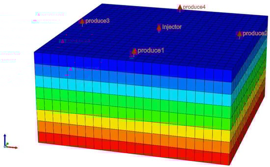
Figure 1.
Three-deminsional diagram of the Water Alternating Gas model.
The key reservoir parameters used in this work are selected based on the geological information of the Tuo 28 block in Shengli Oilfield [33,34], as shown in Table 1. The oil reservoir depth is 1800 m, and the reservoir pressure is 18 MPa due to the normal formation pressure coefficient of 1.0. The reservoir temperature is 85 °C. The porosity is 0.24, the initial oil saturation is 0.7934, the crude oil viscosity is 15.4495 cp, and the crude oil density is 760.9 kg/m3.

Table 1.
Key parameters of the model.
The permeability in the horizontal directions, for each layer from top to bottom, is 10 × 10−3 μm3, 20 × 10−3 μm3, 30 × 10−3 μm3, 40 × 10−3 μm3, 60 × 10−3 μm3, 70 × 10−3 μm3 and 90 × 10−3 μm3, as shown in Table 2, and the average permeability in horizontal directions is 50 × 10−3 μm3. The permeability in the vertical direction is 0.1 times the horizontal permeability (Kv/Kh = 0.1) and the average permeability in the vertical direction is 5 × 10⁻³ μm3, which is a typical non-homogeneous low permeability reservoir with a positive rhythm. The thickness of the whole reservoir is 27 m, with each layer measuring 3 m.
Table 2.
Permeability in horizontal and vertical directions.
2.1.2. Injection and Production Settings
The model simulates a total of forty years, with depletion development occurring during the first eight years and CO2-WAG production commencing in the ninth. Thus, the actual CO2-WAG development length is 32 years. In this case, to compare the production effects of each CO2-WAG scenario, it is necessary to carry out a period of depletion development first to exclude the natural energy disturbance. As shown in Figure 2, the pressure difference between the injection and production wells is less than 0.5 MPa after the first 8 years of depletion development. In addition, the production efficiency is low and no longer productive. Therefore, it is necessary to add energy, such as through CO2-WAG development. In the base model, CO2 injection starts in January of the ninth year and water injection starts in July, so the cycle is set to 12 months, including 6 months of gas injection and 6 months of water injection. The water–gas ratio is set to 1:1, which implies that the CO2 injection rate is equal to the water injection rate under reservoir conditions. The water injection rate is set at 90 m3/day and the CO2 injection rate is set at 20,000 m3/day. The bottom hole pressure of the four production wells is set to 7 MPa. As shown in Figure 3, the water cut in the produced fluid is more than 80% by the fortieth year of production. Thus, this work assumes that production is stopped after 40 years of production.
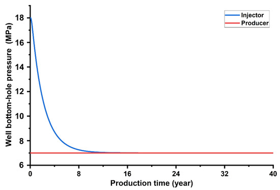
Figure 2.
Bottom-hole pressure in injection and production wells.
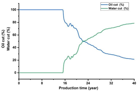
Figure 3.
Oil cut and water cut of the produced fluid in the standard condition.
2.2. Machine Learning for CO2-WAG Prediction
2.2.1. Principle of the Random Forest Regression Algorithm
Multiple regression decision trees constitute the random forest regression algorithm. Based on the idea of integrated learning, the mean value of each regression decision tree is taken as the prediction result [35].
where: is the model prediction result, is the output based on and , is the independent variable, is the independent identically distributed random vector, and is the number of regression decision trees.
As a machine learning algorithm based on statistical theory, the random forest regression algorithm introduces the bagging method and the random subspace method [36] to avoid the problem of single decision tree models, which tend to be overfitted and not accurate.
(1) The bagging method [37], also known as bootstrap aggregating, is a bootstrap-based statistical method. Based on repeatable random sampling, multiple predictors are formed by the bootstrap repetitive sampling method. Assuming that there are N samples in the original sample, N samples are repeatedly sampled to form new training samples. When N approaches infinity, the probability of not being sampled again for each sample is 36.8%. Nearly 36.8% of the original samples will not appear in the training samples of the same tree, and the samples that are not drawn are called out-of-bag data (OOB) [27]. The generation of locally optimal solutions for regression decision trees can be avoided by the bagging method.
(2) Stochastic subspace method. Random features need to be selected when constructing the regression decision tree. Selecting random features means picking x feature attributes at random from the whole set of attributes. Node splitting selects the optimal features based on the principle of minimum mean squared deviation so that each tree is not pruned to achieve maximum growth. A random sampling of training samples and a random selection of feature attributes can make sure that the regression decision trees have as much variety as possible [38].
2.2.2. Randomized Regression Forest Algorithm Flow
The main flow of the randomized regression forest algorithm is presented in Figure 4 and described as follows:
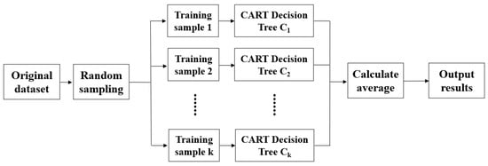
Figure 4.
The training process of the random forest algorithm.
(1) Sampling: K sets of datasets are sampled from the training dataset S by using the bagging method. Each set of datasets is divided into 2 types: sampled data and un-sampled data (out-of-bag data), and they are trained to produce a decision tree.
(2) Growing: Each decision tree is trained by training data. In each branching node, M features are randomly selected from M feature attributes, and the best features are chosen based on the Gini index for full branching growth until no more growth is possible without pruning.
(3) Forming a forest: Repeat steps 1 and 2 to build multiple regression decision trees and maximize the growth of each tree to form a forest.
(4) Predicting: Using the chosen model, predictions are made about the new data set, and the final output is the average of all the predictions made by the decision trees.
This work first builds a series of numerical simulation models by adjusting the injection parameters and runs them to obtain simulation results for forming a test database. The train_test_split function from sklearn.model_selection is called to randomly divide the test database into two parts, one as a training set to train the regression prediction model and the other as a test set to compare with the results predicted by machine learning to verify the accuracy of the method. To make the results clearer and more intuitive, this work trains and predicts each of the three label variables separately with the random forest regression algorithm.
The CO2-WAG period, fluid injection rate, and water–gas ratio are important parameters for CO2-WAG optimization. Therefore, this work uses CO2-WAG period, CO2 injection rate and water–gas ratio as three features and cumulative oil production, CO2 storage amount, and CO2 storage efficiency as labels for regression prediction to realize fast prediction of program effects with the help of a random forest regression algorithm in machine learning.
3. Results and Discussion
3.1. Base Case Analysis
The cumulative oil production, CO2 storage amount, and CO2 storage efficiency of the base model as a function of time are shown in Figure 5 and Figure 6. The values of cumulative oil production, CO2 storage amount, and CO2 storage efficiency are derived as the three labels for machine learning. The CO2 storage amount is obtained by subtracting the cumulative CO2 production from the cumulative CO2 injection. The CO2 storage efficiency is expressed as the ratio of the CO2 storage amount to the CO2 injection.

Figure 5.
Cumulative oil production in the production process.


Figure 6.
CO2 storage in the production process: (a) injection, production and storage amount of CO2, and (b) CO2 storage efficiency.
As shown in Figure 5, at first, the oil production rate goes up quickly because there is enough energy in the reservoir. As the reservoir energy gradually depletes, the oil production curve begins to level off gradually in the fifth year. Then, the reservoir energy is replenished by the nineth year after the CO2-WAG started, and the oil production rate begins to increase rapidly. The oil production rate begins to decrease slowly from the twentieth year to the end of production.
At the beginning of the CO2 injection, the CO2 storage amount is almost equal to the CO2 injection amount from the nineth year to the fifteenth year with little CO2 produced (Figure 6a). CO2 production begins in the fifteenth year and has a relatively stable rate. From the sixteenth year, the growth rate of CO2 storage starts to be lower than that of CO2 injection. With the increase in CO2 production, the CO2 storage amount nearly stopped increasing by the thirty-sixth year. Consequently, the CO2 storage efficiency is almost equal to 1 at the beginning and then gradually decreases, as shown in Figure 6b.
As shown in Figure 7, the overall effects of oil production on both CO2 flooding and CO2-WAG are higher than those of water flooding. CO2 flooding has higher oil production in the early stages of development before the thirty-sixth year because CO2 is more mobile than water. CO2 flooding produces oil at a higher rate than both water flooding and CO2-WAG at this stage. Due to the heterogeneity of the reservoir, the CO2 injected into the formation tends to form a dominant channel. So, the CO2 flooding method starts to produce more oil in a slow way around the twenty-second year of its late stage of development. The CO2-WAG method effectively combines the advantages of water flooding and CO2 flooding and maintains a high oil production rate, especially after the thirty-sixth year, although the oil production rate is relatively lower than that of CO2 flooding before the thirty-sixth year. The overall oil production of CO2-WAG is better than that of water flooding and CO2 flooding.
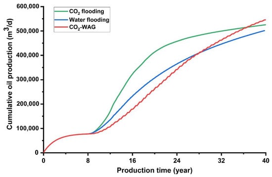
Figure 7.
Cumulative oil production of CO2-WAG, CO2 flooding and water flooding.
For further analysis of the difference between the CO2-WAG method and the CO2 flooding method, this work compares the gas–oil ratio of the produced flow. As shown in Figure 8, the gas production rate starts to increase from the twelfth year (4 years after CO2 injection) in the CO2 flooding method and rises sharply from the nineteenth year onwards. This can be explained by the fact that the injected CO2 forms a dominant channel, and thus the injected CO2 returns to the surface directly from the dominant channel as an output gas.
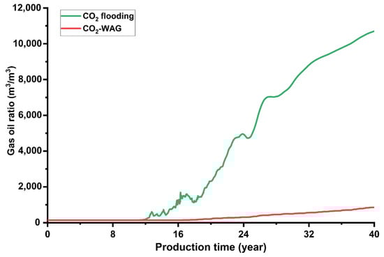
Figure 8.
Gas oil ratio of the production in the WAG and CO2 flooding.
In the CO2-WAG method, the gas production rate is basically unchanged in the early stage of production and increases at a low rate in the late stage of production. Thus, the gas production volume is much smaller than that of CO2 flooding. It can be speculated that the injected water in the CO2-WAG method effectively hinders the breakthrough of CO2 and the formation of a CO2-dominant channel. Therefore, CO2-WAG can effectively slow down the rate of CO2 gas extraction compared to CO2 flooding.
Currently, the treatment and separation of output gas to recover methane and reinjected carbon dioxide are priorities for many oilfields. Gas treatment stations in oilfields have a certain upper limit of gas that can be processed per day. In the CO2 flooding method, the gas output rate may be too high, especially in the final stages of development. It may lead to a risk that a large amount of methane gas and carbon dioxide cannot be captured and recovered in time, causing a great loss of economic benefits and more emissions of greenhouse gases. In contrast, according to the preceding analysis, the CO2-WAG method can solve the aforementioned issues by efficiently extracting crude oil and reducing the gas production rate, thereby allowing the gas treatment station sufficient time to capture and recover methane gas and reinject carbon dioxide.
3.2. Analysis of Influence Factors on CO2-WAG
To analyze the principal influence factors of CO2-WAG, this work designs a series of scenarios of the CO2-WAG development method by modifying the CO2-WAG period, fluid injection rate, and water–gas ratio based on the above base model. Among them, six schemes of the period adjustment are set as 4 months, 6 months, 12 months, 24 months, 48 months, and 96 months, respectively. Six schemes of the fluid injection rate adjustment are set as: (1) water injection rate of 65 m3/day and CO2 injection rate of 12,000 m3/day; (2) water injection rate of 79 m3/day and CO2 injection rate of 16,000 m3/day; (3) water injection rate of 90 m3/day and CO2 injection rate of 20,000 m3/day; (4) water injection rate of 100 m3/day and CO2 injection rate of 23,000 m3/day; (5) water injection rate of 110 m3/day and CO2 injection rate of 27,000 m3/day; (6) water injection rate 120 m3/day and CO2 injection rate of 31,000 m3/day. 6 schemes of the water–gas ratio adjustment are set as 0.33, 0.5, 1, 1.5, 2, and 3, respectively. Therefore, this work constructs a total of 6 × 6 × 6 = 216 scenarios. As the water injection rate varies simultaneously with the CO2 injection rate, this work selects the CO2 injection rate as one feature, and the period and water–gas ratio as the other two features.
The cumulative oil production, CO2 storage amount, and CO2 storage efficiency of the 216 scenarios are simulated by CMG, and the results are detailed in Supporting Information. To elucidate more clearly the influence of CO2-WAG parameters on production, the cumulative oil production, CO2 storage amount, and CO2 storage efficiency of different cycle schemes (#85, #97, #103), different fluid injection rate schemes (#49, #121, #193), and different water–gas ratio schemes (#85, #87, #89) are compared by the single variable method, and the results are shown in Figure 9, Figure 10 and Figure 11.

Figure 9.
Effect of WAG cycle on (a) cumulative oil production, (b) CO2 storage amount, and (c) CO2 storage efficiency.

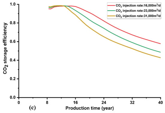
Figure 10.
Effect of fluid injection rate on (a) cumulative oil production, (b) CO2 storage amount, and (c) CO2 storage efficiency.
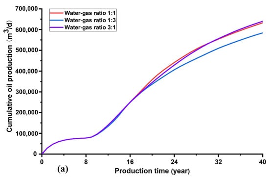
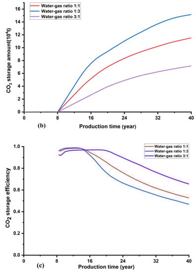
Figure 11.
Effect of water–gas ratio on (a) cumulative oil production, (b) CO2 storage amount, and (c) CO2 storage efficiency.
As shown in Figure 9, the influence of the cycle on oil production is relatively small. When the CO2-WAG cycle is relatively shorter, the cumulative oil production is higher. When the cycle is 8 years, the cumulative oil production starts to decline significantly, because in this case, the frequency of alternating water and carbon dioxide is low, similar to a small period of water flooding and gas flooding. The influence of the cycle on CO2 storage is relatively large, both in terms of CO2 storage amount and CO2 storage efficiency. Throughout the production process, CO2 storage amount and CO2 storage efficiency fluctuate due to the alternate injection of water and CO2. At the end of the process, the CO2 storage amount and CO2 storage efficiency decrease with the cycle.
As shown in Figure 10, the injection rate has a greater impact on oil production. As the injection rate increases, cumulative oil production also increases, but the CO2 storage efficiency decreases. This is because more CO2 will return to the surface from production wells as output gas when the CO2 injection rate increases. Therefore, when optimizing the CO2-WAG extraction scheme in the oilfield, the injection rate cannot be increased arbitrarily. The processing capacity of gas treatment stations in the oilfield needs to be considered. When CO2 output is too fast, some CO2 will not be recovered and treated in time. CO2 will escape into the atmosphere, which may cause environmental issues and aggravate the greenhouse effect. It also causes waste of CO2 gas resources and economic loss to the oilfield. At the same time, an over-high injection rate will instantly increase the bottom hole pressure of the injection well. When it exceeds the fracture pressure of the formation, it will crush the formation, causing damage to the formation on the one hand. On the other hand, it may cause CO2 to escape and pollute other formations.
The model in this study has a low reservoir pressure due to a period of depleted extraction in the early stage. In addition, the fluid injection rate is low, which means it cannot restore the reservoir pressure to the initial pressure. The simulated reservoir is a low-pressure reservoir. For this type of reservoir, as shown in Figure 11, the higher the water–gas ratio is, the better the oil production will be. In addition, when the injection rate and the reservoir pressure are high, a lower water–gas ratio has a higher oil recovery. A higher water–gas ratio results in less CO2 being buried because the proportion of injected CO2 is smaller, but the storage efficiency is higher. A lower water–gas ratio allows more CO2 to be buried because the proportion of CO2 in the injected fluid is larger. Moreover, more CO2 will be produced from the production well, leading to lower storage efficiency.
3.3. Analysis of Machine Learning Results
To compare the CMG numerical simulation results with the machine learning regression prediction results, this work builds a database of 216 CMG numerical simulation models, of which 70% are used as the training set and 30% as the test set. The numerical simulation results of the test set are employed as the true values for verifying the accuracy of the machine learning prediction. The result plots for the three labels of cumulative oil production, CO2 storage amount, and CO2 storage efficiency are shown in Figure 12. The predicted curve made by the random forest regression algorithm is very close to the true value curve in terms of cumulative oil production, CO2 storage amount, and CO2 storage efficiency.
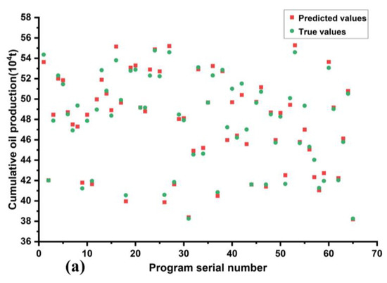
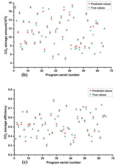
Figure 12.
Comparison of the predicted values by random forest algorithm with the true values in (a) cumulative oil production, (b) CO2 storage amount, and (c) CO2 storage efficiency.
The relative deviation of cumulative oil production, CO2 storage amount, and CO2 storage efficiency for each scheme are calculated and shown in Figure 13 for further discussion. The relative deviation of cumulative oil production between prediction and true values ranges from −4.76% to 2.51%, the maximum relative deviation is −4.76%, and the average absolute relative deviation is 1.10%. The maximum relative deviation of CO2 storage amount between prediction and true values is −15.15%. Except for this, the relative deviation for all other scenarios ranges from −10.67% to 5.23%. The average absolute relative deviation for predicting CO2 storage amount is 3.04%. For the prediction of CO2 storage efficiency, except for three scenarios with large relative deviations of −13.35%, −11.93%, and 8.72%, respectively, the relative deviation for all other scenarios ranges from −6.31% to 4.55%. The average absolute relative deviation for predicting CO2 storage efficiency is 2.24%.
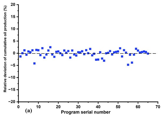

Figure 13.
Relative deviation between the predicted value and true value in (a) cumulative oil production, (b) CO2 storage amount, and (c) CO2 storage efficiency.
According to the curve between the predicted value and the true value, and their relative deviation, the random forest regression algorithm can accurately predict the CO2-WAG production. Therefore, the cumulative oil production, CO2 storage amount, and CO2 storage efficiency can be accurately estimated by this method for the cases of various periods, fluid injection rates, and water–gas ratios.
Moreover, compared to the simulation method, the machine learning-assisted prediction method can save the time of adjusting the CMG model and running data files. It takes about 30 s to run a case of the CMG model and 108 min for all of the 216 cases in this study. The machine learning method employed in this work only spends 10 s predicting all of the scenarios, which shows a big advantage in computational efficiency compared to the CMG simulation method. If the grid of the CMG model is refined, the timesaving advantage of the machine learning method will be much huger. Therefore, the machine learning-assisted method can greatly improve the prediction efficiency of CO2-WAG and will be suitable for injection parameter optimization.
4. Conclusions
For the application of CO2-WAG used in non-homogeneous, low-permeability reservoirs and the machine learning-assisted prediction method of CO2-WAG, some conclusions can be drawn from this work as follows:
(1) Compared to water flooding and continuous CO2 flooding, CO2-WAG can effectively improve oil recovery. In addition, compared to CO2 flooding, CO2-WAG can reduce the CO2 production rate, which is conducive to the storage of CO2 for the reduction of greenhouse gas emissions.
(2) The CO2-WAG cycle time has a slight influence on oil production. Both CO2 storage amount and CO2 storage efficiency decrease with the cycle. On the premise that the reservoir formation is not fractured, the oil production increases but CO2 storage efficiency decreases with the fluid injection rate. For low-pressure reservoirs, the oil production increases with the water–gas ratio, but CO2 storage efficiency decreases with the water–gas ratio.
(3) The random forest regression algorithm in machine learning has better fitting accuracy in predicting the results of CO2-WAG development. Therefore, it can be used to predict the oil production and CO2 storage results under different combinations of injection parameters.
(4) Compared to numerical simulations, using machine learning algorithms to predict results avoids the need to build models and run data files, which will save a lot of time for subsequent parameter optimization.
Supplementary Materials
The following are available online at https://www.mdpi.com/article/10.3390/app122110958/s1.
Author Contributions
Conceptualization, H.L.; Data curation, C.G.; Formal analysis, C.G.; Funding acquisition, H.L., J.X. and S.L.; Investigation, C.G.; Methodology, H.L. and C.G.; Project administration, H.L. and S.L.; Software, C.G.; Supervision, S.L.; Writing—original draft, H.L. and C.G.; Writing—review & editing, H.L., S.L., J.X. and G.I. All authors have read and agreed to the published version of the manuscript.
Funding
This research was funded by the National Natural Science Foundation of China [52074337, 51906256, 52174052, 51904323], the Shandong Provincial Natural Science Foundation [ZR2021JQ18] and Fundamental Research Funds for the Central Universities [21CX06033A].
Institutional Review Board Statement
Not applicable.
Informed Consent Statement
Not applicable.
Data Availability Statement
All data is involved in the text.
Acknowledgments
This research is supported by the National Natural Science Foundation of China, the Shandong Provincial Natural Science Foundation and Fundamental Research Funds for the Central Universities, which are gratefully acknowledged.
Conflicts of Interest
The authors declare no conflict of interest.
References
- Gao, J.; Lv, J. Problem analysis on low permeability reservoir water flooding. Inn. Mong. Petrochem. Ind. 2009, 48–51. [Google Scholar]
- Li, S.; Tang, Y. Present situation and development trend of CO2 injection enhanced oil recovery technology. Oil Gas Reserv. Eval. Dev. 2019, 9, 1–8. [Google Scholar]
- Chen, H.; Liu, X. Prospects and key scientific issues of CO2 near-miscible flooding. Pet. Sci. Bull. 2020, 3, 392–401. [Google Scholar]
- Liu, S.; Ren, B.; Agarwal, B. CO2 storage with enhanced gas recovery (CSEGR): A review of experimental and numerical studies. Pet. Sci. 2022, 19, 594–607. [Google Scholar] [CrossRef]
- Wei, Q.; Hou, J. Laboratory study of CO2 channeling characteristics in ultra-low-permeability oil reservoirs. Pet. Sci. Bull. 2019, 2, 145–153. [Google Scholar]
- Chen, Z.; Su, Y. Characteristics and mechanisms of supercritical CO2 flooding under different factors in low-permeability reservoirs. Pet. Sci. 2022, 19, 1174–1184. [Google Scholar] [CrossRef]
- Tang, R.; Wang, H. Effect of water and gas alternate injection on CO2 flooding. Fault Block Oil Gas Field 2016, 23, 358–362. [Google Scholar]
- Sanchez, N.L. Management of water alternating gas (WAG) injection projects. In Proceedings of the Latin American and Caribbean Petroleum Engineering Conference, Caracas, Venezuela, 21–23 April 1999. [Google Scholar]
- Christensen, J.R.; Stenby, E.H. Review of WAG field experience. SPE Reserv. Eval. Eng. 2001, 4, 97–106. [Google Scholar] [CrossRef]
- Rochedo, P.R.R.; Costa, I.V.L. Carbon capture potential and costs in Brazil. J. Clean. Prod. 2016, 131, 280–295. [Google Scholar] [CrossRef]
- Godoi, J.M.A.; dos Santos Matai, P.H.L. Enhanced oil recovery with carbon dioxide geosequestration: First steps at Pre-salt in Brazil. J. Pet. Explor. Prod. 2021, 11, 1429–1441. [Google Scholar] [CrossRef]
- Kengessova, A. Prediction efficiency of immiscible Water Alternating Gas Performance by LSSVM-PSO algorithms. Master’s Thesis, University of Stavanger, Stavanger, Norway, 2020. [Google Scholar]
- Mohagheghian, E.; James, L.A. Optimization of hydrocarbon water alternating gas in the Norne field: Application of evolutionary algorithms. Fuel 2018, 223, 86–98. [Google Scholar] [CrossRef]
- Bender, S.; Yilmaz, M. Full-Field Simulation and Optimization Study of Mature IWAG Injection in a Heavy Oil Carbonate Reservoir. In Proceedings of the SPE Improved Oil Recovery Symposium, Tulsa, OK, USA, 12–16 April 2014. [Google Scholar]
- Johns, R.T.; Bermudez, L. WAG optimization for gas floods above the MME. In Proceedings of the SPE Annual Technical Conference and Exhibition, Denver, CO, USA, 5–8 October 2003. [Google Scholar]
- Chen, S.; Li, H. Optimal parametric design for water-alternating-gas (WAG) process in a CO2-miscible flooding reservoir. J. Can. Pet. Technol. 2010, 49, 75–82. [Google Scholar] [CrossRef]
- Mousavi Mirkalaei, S.M.; Hosseini, S.J. Investigation of Different I-WAG Schemes Toward Optimization of Displacement Efficiency. In Proceedings of the SPE Enhanced Oil Recovery Conference, Kuala Lumpur, Malaysia, 19–21 July 2011. [Google Scholar]
- Ghaderi, S.M.; Clarkson, C.R. Evaluation of recovery performance of miscible displacement and WAG process in tight oil formations. In Proceedings of the SPE/EAGE European Unconventional Resources Conference and Exhibition, Vienna, Austria, 20–22 March 2012. [Google Scholar]
- You, J.; Ampomah, W. Assessment of Enhanced Oil Recovery and CO2 Storage Capacity Using Machine learning and Optimization Framework. In Proceedings of the SPE Europec featured at 81st EAGE Conference and Exhibition, London, England, UK, 3–6 June 2019. [Google Scholar]
- Zhou, D.; Yan, M. Optimization of a mature CO2 flood—From continuous injection to WAG. In Proceedings of the SPE Improved Oil Recovery Symposium, Tulsa, OK, USA, 14–18 April 2012. [Google Scholar]
- Rodrigues, H.; Mackay, E.; Arnold, D.; Silva, D. Optimization of CO2-WAG and Calcite Scale Management in Pre-Salt Carbonate Reservoirs. In Proceedings of the Offshore Technology Conference Brasil, Rio de Janeiro, Brazil, 29–31 October 2019. [Google Scholar]
- Min, C.; Dai, B. A Review of the Application Progress of Machine Learning in Oil and Gas Industry. J. Southwest Pet. Univ. 2020, 42, 1–15. [Google Scholar]
- He, Y.; Song, Z. Application of machine learning in hydraulic fracturing. J. China Univ. Pet. 2021, 45, 127–135. [Google Scholar]
- Bilgesu, H.I.; Al-Rashidi, A.F. An unconventional approach for drill-bit selection. In Proceedings of the SPE Middle East Oil Show, Manama, Bahrain, 17–20 March 2001. [Google Scholar]
- Leite Cristofaro, R.A.; Longhin, G.A. Artificial Intelligence Strategy Minimizes Lost Circulation Non-Productive Time in Brazilian Deep Water Pre-Salt. In Proceedings of the OTC Brasil, Rio de Janeiro, Brazil, 24–26 October 2017. [Google Scholar]
- Wang, W.; Shi, M. Joint optimization method of well location and injection-production parameters based on machine learning. J. Shenzhen Univ. 2022, 39, 126–133. [Google Scholar]
- Breiman, L. Random forests. Mach. Learn. 2001, 45, 5–32. [Google Scholar] [CrossRef]
- Feng, M.; Yan, W. Predicting Total Organic Carbon Content by Random Forest Regression Algorithm. Bull. Mineral. Petrol. Geochem. 2018, 37, 475–481. [Google Scholar]
- Zhen, Y.; Hao, M. Research of medium and long term precipitation forecasting model based on random forest. Water Resour. Power 2015, 33, 6–10. [Google Scholar]
- Wang, P.; Lu, B. Water demand prediction model based on random forests model and its application. Water Resour. Prot. 2014, 30, 34–37. [Google Scholar]
- Lv, H.; Feng, Q. A review of random forests algorithm. J. Hebei Acad. Sci. 2019, 36, 37–41. [Google Scholar]
- Du, X.; Feng, J. PM2.5 concentration prediction model based on random forest regression analysis. Telecommun. Sci. 2017, 33, 66–75. [Google Scholar]
- Zhang, Y. The Study on Reservoir Description and Remaining Oil Distribution on the 4th–6th Sandstone Beds of the Second Member in the Shahejie Formation of Tuo 28 Block in Shengtuo Oilfield; China University of Petroleum: Qingdao, China, 2017. [Google Scholar]
- Miao, C. Reservoir Description on the 1st–3rd Sandstone Beds of the Second Member in the Shahejie Formation of the Tuo 28 Block in Shengtuo Oilfield; China University of Petroleum: Qingdao, China, 2016. [Google Scholar]
- Cutler, A.; Cutler, D.R.; Stevens, J.R. Random Forests. In Ensemble Machine Learning; Zhang, C., Ma, Y., Eds.; Springer: Boston, MA, USA, 2012. [Google Scholar]
- Fang, K.; Wu, J. A Review of Technologies on Random Forests. J. Stat. Inf. 2011, 26, 32–38. [Google Scholar]
- Hillebrand, E.; Lukas, M. Bagging weak predictors. Int. J. Forecast. 2021, 37, 237–254. [Google Scholar] [CrossRef]
- Criminisi, A.; Shotton, J. (Eds.) Decision Forests for Computer Vision and Medical Image Analysis; Springer Science & Business Media: Berlin/Heidelberg, Germany, 2013. [Google Scholar]


Publisher’s Note: MDPI stays neutral with regard to jurisdictional claims in published maps and institutional affiliations. |
© 2022 by the authors. Licensee MDPI, Basel, Switzerland. This article is an open access article distributed under the terms and conditions of the Creative Commons Attribution (CC BY) license (https://creativecommons.org/licenses/by/4.0/).