Abstract
Condition monitoring of gear train assembly has been carried out with vibration signals acquired from an all-terrain vehicle (ATV) gearbox. The location of the defect in the gear was identified based on finite element analysis results. The vibration signals were acquired using an accelerometer under good and simulated fault conditions of the gear. The raw vibration signatures acquired from all the possible conditions of the gear train assembly were processed using the descriptive statistics tool. A set of descriptive statistical features were extracted from the raw vibrational signals. This study used a deep learning algorithm based on the tree family, which includes the decision tree, random forest, and random tree algorithms, to classify gear train conditions. Among the tree family algorithms, the random forest algorithm produced maximum classification accuracy of 99%. The decision rules were used to design an online monitoring system to display the gear condition. This study will help to implement online gear health monitoring in ATVs, ensuring the safety of drivers.
1. Introduction
Gears are the essential parts of the power transmission system of automotive vehicles. A geartrain assembly provides different torque and speed combinations for uniform power on varying road conditions [1]. Hence, fault diagnosis of a gear train assembly is an essential process for identifying gear failures during their operation. The gear stiffness determines the flexibility of the tooth, and defects in the gears result in variable gear stiffness and mesh frequency, which cause the vibration pattern of the gear assembly to vary [2]. Vibration analysis is the most communal means of predictive gear maintenance and fault diagnostics [3]. Although faults influence gear vibration in gear train assembly, the vibration signals are usually captured at the gear train casing, which is also influenced by other parts of the vehicle, such as the chassis and the engine of ATVs [4]. The acquired vibration data may be in the form of a time domain, frequency domain, and time–frequency domain [5]. Acoustic emission and vibration signals significantly affect gearbox conditions [6].
Various methods, such as spectral analysis, power cepstrum analysis, cyclo-stationary processes, time-synchronous average methods, etc., can be used to process the vibration signals to identify the faults in gears [7,8]. Statistical [9], histogram [10], and wavelet transform [11] are approaches that can be used for analyzing the signals logically with programming functions. Statistical feature extraction is one of the frequently used time-domain signal-processing approaches through which the raw vibration signals are decomposed into small segments of information called features [12]. This study also extracted statistical features using Visual Basic.
The extracted features comprise the source data for classifying the condition of the gear train. There are many algorithmic approaches available for analyzing the extracted statistical features. The tree family algorithm is one of the most efficient methods to analyze vibration data with better accuracy. Earlier, among the performances of various deep learning algorithms, decision trees were found to be more accurate in detecting faults [13]. The decision tree algorithm was used to analyze the statistical features of vibration signals for misfires in an internal combustion engine [14,15]. Additionally, the same classifier algorithm was used to analyze the vibration signals due to the faulty gearbox [16] and cutting tool wear [11]. The accuracy of the statistical analysis obtained after post-pruning the decision tree was higher than the C4.5 decision tree [17]. In another study, the defects in a helical gearbox of a commercial vehicle were recognized using the decision tree algorithms [18].
Gear pitting is the most commonly occurring fault in the power transmission system. A test rig was used for the experiments, and vibration signals were captured. A deep learning algorithm was used to monitor the pitting level [19]. Gear pitting can also be monitored using vibration, current, and AE signals [20]. A detailed summary of studies that applied machine learning algorithms for fault monitoring was reviewed [21]. The application of deep learning algorithms in fault diagnosis of various rotating elements was discussed [22,23]. Fault diagnosis of a gearbox was performed with a standard gear, a gear with wear and tear, a gear with cracks, a gear with broken teeth, and a gear with tooth deficiency conditions. A deep learning algorithm was used to monitor gear health [24].
As listed in the literature, all the diagnosis applications were reported using test setups. Many studies have been reported for a single-stage spur gear assembly and a single-stage helical gear assembly. A gear was tested in the rig with seven different gear pitting conditions, and AE and vibration signals were captured. Convolutional neural network (CNN) and gated recurrent unit (GRU) networks were integrated to monitor gear health [25]. The condition of the worm gearbox was monitored with thermal images using a deep learning algorithm [26]. However, no studies have been reported to monitor the condition of a real-time two-stage gear train fitted with an ATV. In this study, a gear train assembly has been considered for condition monitoring applications. The tree family algorithms, such as the random tree, random forest, and decision tree algorithms, were used to make a comparative study. The flow chart representing the data collection is represented in Figure 1.
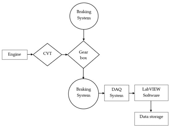
Figure 1.
Flow chart for data collection.
2. Experimental Setup
Figure 2a shows the ATV used for this study. The vibration signatures were taken on an experimental setup shown in Figure 2b. The gear train setup consists of a Briggs and Stratton Model 19 Engine (7.5 HP) with a maximum speed of up to 3800 RPM coupled with the gear train assembly via a continuously variable transmission (CVT). Theoretically, the CVT has an infinite gear ratio which helps to control the speed and torque of the vehicle. The CVT is interconnected with a Kevlar belt which minimizes the shock loading which emanates from the engine.
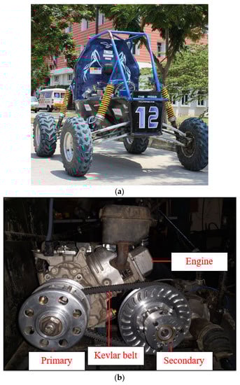
Figure 2.
(a) ATV used for experiments. (b) Power train setup.
The two-stage gear train consisted of spur gears in the first stage and helical gears in the second stage. The schematic representation of the gear train is shown in Figure 3a. The actual gear train is shown in Figure 3b. The gearbox’s output shaft was coupled to the transaxle, which ultimately drives the vehicle. The gear train was fully lubricated with GL490 oil. Mechanical brakes using tandem cylinders were used to apply a load of 280 N for the testing conditions of 1800 and 2000 RPM to account for the road resistance acting during the runtime of the vehicle.
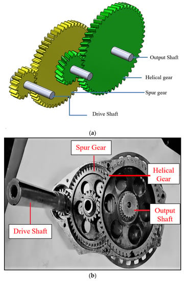
Figure 3.
(a) Schematic representation of gear train assembly. (b) Gear train assembly.
The gear train was considered free from other defects, such as shaft misalignment, bearing, and casing. The only defects induced are on the spur and helical gears while their mating pinions remain unscathed. The vibration signals for all the conditions were obtained using an accelerometer mounted directly on top of the gear train casing, as depicted in Figure 4a,b.
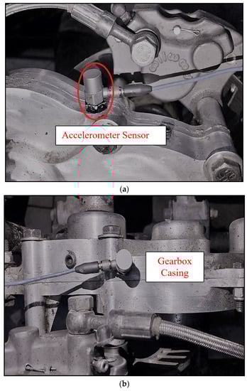
Figure 4.
(a) Sensor mounting (front view). (b) Sensor mounting (top view).
3. Experimental Procedure
The two-stage gear train assembly was modeled with the dimensions of the gears, as shown in Table 1, to identify the gear failure locations. Figure 5 shows the finite element analysis (FEA) of a gear. After the application of load, the bottom of the teeth becomes affected. FEA results reveal that obtained von Mises stress is in the permissible range. Based on this simulated study, the location of the fault was identified, and different faults mentioned in Table 2 were simulated. The size of the defects induced in the gears is slightly larger than those that will present themselves in a real-time scenario after being under load for a prolonged period. Cracks originating at the gear surface may lead to failure modes such as pitting and tooth breakage. Furthermore, the contact load on the flank surface induces stresses at the bottom of the tooth, which may lead to crack initiation. Over time the sub-surface crack propagation may lead to gear failure, referred to as “tooth breakage” [27]. Different crack growth models can estimate crack propagation [28].

Table 1.
Spur and helical gear parameters.
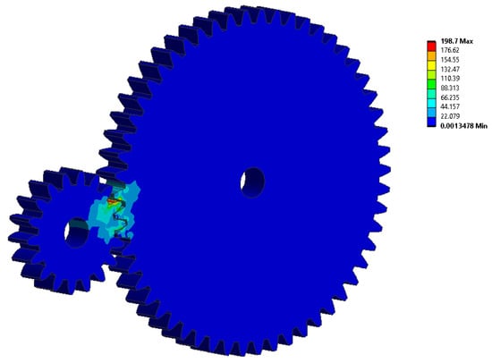
Figure 5.
Finite element analysis of spur gear.
Table 2.
Gear combinations and fault conditions.
Most often, the gear fails due to fatigue and overload. The most common form of failure is actual breakage, and other failure modes include surface fatigue, pitting, normal and abnormal wear, and plastic flow [29]. As per our knowledge, in ATVs, the applied load is significantly less. Hence, the occurrence of the abovementioned failures may be significantly less. The different defects have been collected from the authorized service person. Based on the data collected, the following fault conditions, namely spur and helical gear in healthy condition (SHHC), spur gear with crack (SGWC), spur gear with broken tooth (SGBT), helical gear with crack (HGWC), helical gear with broken tooth (HGBT), and helical and spur gear with broken tooth (HSBT) were simulated on the gear. Figure 6a–d show the instigated defects for spur and helical gears.
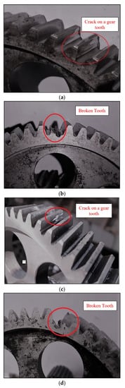
Figure 6.
(a) Crack on the tooth of spur gear. (b) Spur gear with a broken tooth. (c) Crack on the tooth of helical gear. (d) Helical gear with a broken tooth.
In the experimental setup, different gear sets were used for every condition of the gears. The combination of gears used in the gearbox is mentioned in Table 2. The vibration signals were taken for three engine shaft speeds (1500, 1800, and 2000 RPM). The loading condition (0 N and 280 N) provided for 1800 and 2000 RPM to account for the rolling resistance encountered during the runtime of the vehicle.
The vibration signals were collected with the help of an accelerometer (a piezo-ceramic sensing element) placed on the casing of the gear train assembly. The signals were taken after allowing the gearbox to run for a little while. The sample length was arbitrarily chosen as 10,000, and the sampling frequency was set at 25 kHz for all conditions. Generally, a large sample size ensures more accurate statistical measures. On the contrary, a large sample size would mean longer computational time. To find a solution to this problem, a sample size of 10,000 was decided. Many trial runs were conducted at one set speed, and the vibrational signals were recorded when the engine attained the optimum running conditions. A hundred data files containing 10,000 samples were considered for the analysis of each simulated condition of the gearbox.
4. Feature Extraction and Feature Selection
The raw vibration signals were acquired from the gear train under all the faulty conditions simulated (SHHC, SGWC, SGBT, HGWC, HGBT, and HSBT), as shown in Figure 7. The vibrational signals for the above conditions were collected under 0 N and 280 N loading conditions and different engine speeds. The twelve statistical features were extracted from acquired vibration signals [18,30]. Instead of using all the extracted features, the valuable features alone were selected from the extracted features using the effect of several feature selection studies [30]. The order of features was selected using the attribute evaluator [31].
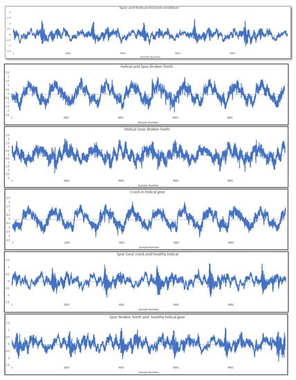
Figure 7.
Vibration signals for different gearbox conditions.
Based on the attribute evaluator, the first feature alone was used for the classification, and the corresponding accuracy will be noted. The second feature suggested by the attribute evaluator was then clubbed with the first feature, and the two-feature set was classified. Then, the third feature clubbed to the previous set, and the results were noted. In the same way, the accuracy was calculated until all the features were added and classified once. Among these, the feature set combination which produced maximum accuracy was selected for further classification.
5. Feature Classification Using the Tree Family Algorithms
The decision tree algorithm utilizes information gain and entropy for making the decision tree with the help of decision rules. The tree model was developed based on the given training data. The decision tree algorithm calculates information gains of all possible branching features, and the one with the highest information gain is selected for further classification [32]. The classification accuracy of the decision tree is demonstrated by its confusion matrix [31]. The confusion matrix of the algorithm recognizes the number of correctly matched and mismatched instances.
The random tree is a supervised learning algorithm broadly used in data mining for classification problems. It generates multiple learners that construct a decision tree [33]. Every node is bifurcated according to the best variable parameters among the available ones. This decision tree constructs a tree consisting of N chosen attributes at a time. The number of attributes chosen is random, out of which the highest entropy gain attribute is selected for further bifurcation until the node class is reached.
The random forest classifier is an aggregate of multiple decision trees that uses a classification and regression tree (CART) for predictive analysis [34]. Random forest uses the random subspace method for improving the estimation by selecting random samples of features instead of the entire feature set [7]. After producing the independent decision trees, each node is split randomly according to the number of features provided by the user. The final classification decision is calculated using the arithmetic mean of the class assignment probabilities of the produced trees [35]. This study used the three tree family algorithms for the classification process.
6. Results and Discussion
The experiment started with six fault conditions of the gear train, as mentioned in Table 2. The vibration signals were recorded at three different speeds for each fault condition of the gear train. For 1500 RPM, no load was applied on the gearbox, whereas for 1800 and 2000 RPM, a constant load of 280 N was applied to account for the road resistances encountered by the gear train during the operating condition, as shown in Table 3. The statistical features were extracted from the vibration signature under each condition. The participating features were selected using the accuracy by class and the attribute evaluator. Three tree algorithms were selected to classify the input features and check the accuracy at each engine speed. Table 4 shows the maximum classification accuracy for 1800 RPM for the random forest; 99% is maximum accuracy. Hence, 1800 RPM was considered for further analysis.
Table 3.
Loading conditions at different speeds.
Table 4.
Effect of number of features studied for the speed of 1800 RPM.
Figure 7 reveals that vibration amplitude is higher for faulty gears than for healthy gears. The increase in vibration is ascribed to the faulty conditions of the gear. Table 5 shows the classification accuracy for all the tree family classifiers: random forest, decision tree, and random tree. The selected features under all the speed conditions were classified using the tree family algorithms, and the corresponding accuracy values are presented in Table 5. In Table 5, the decision tree and random forest produced maximum classification accuracies of 98.33% and 99%, respectively, with seven features. The random tree suggests ten features for the maximum classification accuracy of 98.67%.
Table 5.
Accuracy of the tree family classifiers.
Under each condition, 100 data samples were used for classification. The ten-fold cross-validation was used to obtain the accuracy. From these three trees, it is seen that the maximum accuracy was found as 99% for the random forest algorithm. This can be studied using the confusion matrix obtained from the random forest algorithm. Table 6 shows the confusion matrix obtained from the random forest under a speed of 1800 RPM.
Table 6.
Confusion matrix for random forest algorithm.
The matrix displays the correct and incorrect instances classified by the algorithm. Each column of the matrix determines the predicted class of the input data, whereas each row defines the actual condition of the gearbox associated with the input data. The confusion matrix’s diagonal elements are the values correctly classified in the correct nodes. In the first row, among the 100 data points belonging to SHHC, 98 data points were classified as SHHC, and 2 data points were misclassified as SGWC. In the second row, data belongs to SGWC; 97 data points were correctly classified as SGWC. Two data points were misclassified as SHHC and one data point was misclassified as SGBT.
Similarly, in the last row, among the 100 data points belonging to HSBT, all are correctly classified as HSBT. Hence, there was no misclassification. In this manner, the confusion matrix was used to identify the number of correctly classified data points and misclassified data points, and to classify the trained data and determine the total number of data points that were used for classification. Among the 600 data points belonging to all fault conditions, 594 data points were correctly classified with a classification accuracy of 99.00%.
The above classification accuracy was found using the decision rules. These decision rules were used to design the LabVIEW model based on the conditions defined for selected statistical features. The raw signal data were fed into the LabVIEW model. They identified the condition in which the statistical features belong. Figure 8 shows the LabVIEW program used to develop the online model for analyzing the gear train condition. The advantages of the proposed approach are as follows:
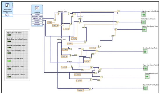
Figure 8.
LabVIEW model for displaying the results.
- ➢
- While driving, any simulated faults in the ATV can be identified immediately.
- ➢
- This study will help implement online gear health monitoring in ATVs, ensuring the safety of drivers.
The model will be tested in real-world systems to make it an online condition monitoring system as the future scope of this study. In the future, other defects such as pitting and scuffing can be considered with dynamic load conditions.
7. Conclusions
The present work has outlined a structure for fault detection in a two-stage gearbox using a vibrational signal; additionally, we applied a deep learning algorithm to characterize the gear train condition of an all-terrain vehicle. The vibration signals were captured from all the simulated good and faulty conditions of the gear train. The statistical features were extracted from the raw vibrational signals using the Visual Basic program. Feature selection and classifications were made using the following tree family algorithms: the decision tree, random forest, and random tree algorithms. The random forest algorithm yielded a maximum classification accuracy of 99.00 % at 1800 RPM. The decision rules were used to design the LabVIEW model for displaying the gear train condition. The model will help display the gear train’s condition as an online model.
Author Contributions
Conceptualization, J.R. and S.G.; methodology, software, M.T.; validation, L.J., S.K.M. and J.R.; formal analysis, K.T.; investigation, J.R.; resources, J.R.; data curation, K.T. and G.K.; writing—original draft preparation, J.R.; writing—review and editing, M.T.; visualization, S.G. and L.J.; supervision, J.R.; project administration, J.R. All authors have read and agreed to the published version of the manuscript.
Funding
This research received no external funding and the APC was funded by VIT University.
Institutional Review Board Statement
Not applicable.
Informed Consent Statement
Not applicable.
Data Availability Statement
Not applicable.
Acknowledgments
The authors thank the Management of VIT University and the Dean-School of Mechanical Engineering, VIT Chennai, Faculty of Centre for Automation, and the Amrita School of Engineering, Coimbatore, Amrita Vishwa Vidyapeetham, India, for their support in publishing this work. Additionally, the authors would like to thank the research scholar Alamelu Manghai T M, who helped acquire the signals.
Conflicts of Interest
The authors declare no conflict of interest.
References
- Zhao, H.; Wu, Q.; Huang, K.; Qiu, M.; Liu, P. Status and problem research on gear study. J. Mech. Eng. 2013, 49, 11–20. [Google Scholar] [CrossRef]
- Rincon, A.F.d.; Viadero, F.; Iglesias, M.; de-Juan, A.; Garcia, P.; Sancibrian, R. Effect of cracks and pitting defects on gear meshing. Proc. Inst. Mech. Eng. Part C J. Mech. Eng. Science 2012, 226, 2805–2815. [Google Scholar] [CrossRef]
- Wang, T.; Han, Q.; Chu, F.; Feng, Z. Vibration based condition monitoring and fault diagnosis of wind turbine planetary gearbox: A review. Mech. Syst. Signal Process. 2019, 126, 662–685. [Google Scholar] [CrossRef]
- Feng, K.; Ji, J.; Ni, Q.; Beer, M. A review of vibration-based gear wear monitoring and prediction techniques. Mech. Syst. Signal Process. 2023, 182, 109605. [Google Scholar] [CrossRef]
- Lei, Y.; Lin, J.; Zuo, M.J.; He, Z. Condition monitoring and fault diagnosis of planetary gearboxes: A review. Measurement 2014, 48, 292–305. [Google Scholar] [CrossRef]
- Praveenkumar, T.; Saimurugan, M.; Ramachandran, K. Intelligent Fault Diagnosis of Synchromesh Gearbox Using Fusion of Vibration and Acoustic Emission Signals for Performance Enhancement. Int. J. Progn. Health Manag. 2019, 10, 1–11. [Google Scholar] [CrossRef]
- Talukdar, S.; Eibek, K.U.; Akhter, S.; Ziaul, S.; Islam, A.R.M.T.; Mallick, J. Modeling fragmentation probability of land-use and land-cover using the bagging, random forest and random subspace in the Teesta River Basin, Bangladesh. Ecol. Indic. 2021, 126, 107612. [Google Scholar] [CrossRef]
- Yuvaraju, E.C.; Rudresh, L.R.; Saimurugan, M. Vibration signals based fault severity estimation of a shaft using machine learning techniques. Mater. Today Proc. 2020, 24, 241–250. [Google Scholar] [CrossRef]
- Sharma, V.; Parey, A. A review of gear fault diagnosis using various condition indicators. Procedia Eng. 2016, 144, 253–263. [Google Scholar] [CrossRef]
- Natarajan, S. Vibration signal analysis using histogram features and support vector machine for gear box fault diagnosis. Int. J. Syst. Control. Commun. 2017, 8, 57–71. [Google Scholar] [CrossRef]
- Mohanraj, T.; Yerchuru, J.; Krishnan, H.; Aravind, R.N.; Yameni, R. Development of tool condition monitoring system in end milling process using wavelet features and Hoelder’s exponent with machine learning algorithms. Measurement 2021, 173, 108671. [Google Scholar] [CrossRef]
- Altaf, M.; Akram, T.; Khan, M.A.; Iqbal, M.; Ch, M.M.I.; Hsu, C.-H. A New Statistical Features Based Approach for Bearing Fault Diagnosis Using Vibration Signals. Sensors 2022, 22, 2012. [Google Scholar] [CrossRef]
- Meena, R.; Nair, B.B.; Sakthivel, N. Machine Learning Approach to Condition Monitoring of an Automotive Radiator Cooling Fan System. In Advances in Electrical and Computer Technologies, Proceedings of the ICAECT 2019: First International Conference in Advances in Electrical and Computer Technologies, Coimbatore, India, 26–27 April 2019; Sengodan, T., Murugappan, M., Misra, S., Eds.; Springer: Berlin/Heidelberg, Germany, 2020; pp. 1007–1020. [Google Scholar]
- Sharma, A.; Sugumaran, V.; Devasenapati, S.B. Misfire detection in an IC engine using vibration signal and decision tree algorithms. Measurement 2014, 50, 370–380. [Google Scholar] [CrossRef]
- Kumar, N.; Sakthivel, G.; Jegadeeshwaran, R.; Sivakumar, R.; Kumar, S. Vibration based IC engine fault diagnosis using tree family classifiers-a machine learning approach. In Proceedings of the 2019 IEEE International Symposium on Smart Electronic Systems (iSES) (Formerly iNiS), Rourkela, India, 16–18 December 2019; pp. 225–228. [Google Scholar]
- Saravanan, N.; Ramachandran, K. Fault diagnosis of spur bevel gear box using discrete wavelet features and Decision Tree classification. Expert Syst. Appl. 2009, 36, 9564–9573. [Google Scholar] [CrossRef]
- Charbuty, B.; Abdulazeez, A. Classification based on decision tree algorithm for machine learning. J. Appl. Sci. Technol. Trends 2021, 2, 20–28. [Google Scholar] [CrossRef]
- Sugumaran, V.; Jain, D.; Amarnath, M.; Kumar, H. Fault diagnosis of helical gear box using decision tree through vibration signals. Int. J. Perform. Eng. 2013, 9, 221. [Google Scholar]
- Li, X.; Li, J.; Qu, Y.; He, D. Semi-supervised gear fault diagnosis using raw vibration signal based on deep learning. Chin. J. Aeronaut. 2020, 33, 418–426. [Google Scholar] [CrossRef]
- Medina, R.; Cerrada, M.; Cabrera, D.; Sánchez, R.-V.; Li, C.; De Oliveira, J.V. Deep learning-based gear pitting severity assessment using acoustic emission, vibration and currents signals. In Proceedings of the 2019 Prognostics and System Health Management Conference (PHM-Paris), Paris, France, 2–5 May 2019; pp. 210–216. [Google Scholar]
- Toh, G.; Park, J. Review of vibration-based structural health monitoring using deep learning. Appl. Sci. 2020, 10, 1680. [Google Scholar] [CrossRef]
- Tama, B.A.; Vania, M.; Lee, S.; Lim, S. Recent advances in the application of deep learning for fault diagnosis of rotating machinery using vibration signals. Artif. Intell. Rev. 2022, 55, 1–43. [Google Scholar] [CrossRef]
- Fu, Q.; Wang, H. A novel deep learning system with data augmentation for machine fault diagnosis from vibration signals. Appl. Sci. 2020, 10, 5765. [Google Scholar] [CrossRef]
- Zhu, X.; Liu, B.; Li, Z.; Lin, J.; Gao, X. Research on Deep Learning Method and Optimization of Vibration Characteristics of Rotating Equipment. Sensors 2022, 22, 3693. [Google Scholar] [CrossRef]
- Li, X.; Li, J.; Qu, Y.; He, D. Gear pitting fault diagnosis using integrated CNN and GRU network with both vibration and acoustic emission signals. Appl. Sci. 2019, 9, 768. [Google Scholar] [CrossRef]
- Karabacak, Y.E.; Gürsel Özmen, N.; Gümüşel, L. Worm gear condition monitoring and fault detection from thermal images via deep learning method. Eksploat. Niezawodn. 2020, 22, 544–556. [Google Scholar] [CrossRef]
- Boiadjiev, I.; Witzig, J.; Tobie, T.; Stahl, K. Tooth flank fracture–basic principles and calculation model for a sub-surface-initiated fatigue failure mode of case-hardened gears. In Proceedings of the International Gear Conference, Lyon, France, 26–28 August 2014; pp. 1–7. [Google Scholar]
- Lewicki, D.G.; Ballarini, R. Gear crack propagation investigations. Tribotest 1998, 5, 157–172. [Google Scholar] [CrossRef]
- Beckman, M. Gear failure analysis. Tribol. Lubr. Technol. 2019, 75, 24–32. [Google Scholar]
- Jegadeeshwaran, R.; Sugumaran, V. Comparative study of decision tree classifier and best first tree classifier for fault diagnosis of automobile hydraulic brake system using statistical features. Measurement 2013, 46, 3247–3260. [Google Scholar] [CrossRef]
- Jegadeeshwaran, R.; Sugumaran, V. Brake fault diagnosis using Clonal Selection Classification Algorithm (CSCA)—A statistical learning approach. Eng. Sci. Technol. Int. J. 2015, 18, 14–23. [Google Scholar] [CrossRef]
- Bhargava, N.; Sharma, G.; Bhargava, R.; Mathuria, M. Decision tree analysis on j48 algorithm for data mining. Proc. Int. J. Adv. Res. Comput. Sci. Softw. Eng. 2013, 3, 1114–1119. [Google Scholar]
- Kalmegh, S.R. Comparative analysis of weka data mining algorithm randomforest, randomtree and ladtree for classification of indigenous news data. Int. J. Emerg. Technol. Adv. Eng. 2015, 5, 507–517. [Google Scholar]
- Javed Mehedi Shamrat, F.; Ranjan, R.; Hasib, K.M.; Yadav, A.; Siddique, A.H. Performance Evaluation Among ID3, C4. 5, and CART Decision Tree Algorithm. In Pervasive Computing and Social Networking, Proceedings of the International Conference on Pervasive Computing and Social Networking(ICPCSN 2021), Salem, India, 19–20 March 2021; Springer: Berlin/Heidelberg, Germany, 2022; pp. 127–142. [Google Scholar]
- Belgiu, M.; Drăguţ, L. Random forest in remote sensing: A review of applications and future directions. ISPRS J. Photogramm. Remote Sens. 2016, 114, 24–31. [Google Scholar] [CrossRef]


Publisher’s Note: MDPI stays neutral with regard to jurisdictional claims in published maps and institutional affiliations. |
© 2022 by the authors. Licensee MDPI, Basel, Switzerland. This article is an open access article distributed under the terms and conditions of the Creative Commons Attribution (CC BY) license (https://creativecommons.org/licenses/by/4.0/).