A Coarse-Grained Molecular Model for Simulating Self-Healing of Bitumen

Abstract

The longevity of asphalt pavements is a key focus of road engineering, which closely relates to the self-healing ability of bitumen. Our work aims to establish a CGMD model and matched force field for bitumen and break through the limitations of the research scale to further explore the microscopic mechanism of bitumen self-healing. In this study, a CGMD mapping scheme containing 16 kinds of beads is proposed, and the non-bond potential energy function and bond potential energy function are calculated based on all-atom simulation to construct and validate a coarse-grained model for bitumen. On this basis, a micro-crack model with a width of 36.6nm is simulated, and the variation laws of potential energy, density, diffusion coefficient, relative concentration and temperature in the process of bitumen self-healing are analyzed with the cracking rate parameter proposed to characterize the degree of bitumen crack healing. The results show that the computational size of the coarse-grained simulation is much larger than that of the all-atom, which can explain the self-healing mechanism at the molecular level. In the self-healing process, non-bonded interactions dominate the molecular movement, and differences in the decreased rate of diffusion among the components indicate that saturates and aromatics play a major role in self-healing. Meanwhile, the variations in crack rates reveal that healing time is inversely proportional to temperature. The impact of increasing temperature on reducing healing time is most obvious when the temperature approaches the glass transition temperature (300 K).

1. Introduction

Bitumen has the ability to self-heal. Microcracks produced by low temperatures and traffic load can be gradually repaired by surface reconstruction, surface proximity, surface wetting, and mutual diffusion. At present, the majority of bitumen self-healing behavior research is based on macroscopic tests, where the healing degree is evaluated by testing the physical properties of the bitumen. However, the self-healing behavior of bitumen is essentially determined by its microscopic properties. Therefore, to really comprehend the self-healing mechanism, emphasis must be paid to the molecular structure of bitumen. For this reason, bitumen research is increasingly using Molecular Dynamics (MD). Initially, Zhang and Greenfield [1] proposed a three-component molecular model of bitumen and, subsequently, Li and Greenfield [2,3] a four-component model. Researchers have investigated the mechanism of self-healing using these molecular models. Scanning electron microscope imaging of bitumen microcracks in combination with MD simulations by Shen et al. [4] demonstrated that temperature, crack width, and the degree of aging are major factors affecting self-healing. Sun et al. [5] determined an optimal self-healing temperature, while Qu et al. [6] proposed a six-component model of a bitumen healing agent. It was found that crack width, temperature, state of molecular aggregation, and aggregate influence self-healing. He et al. [7,8] performed MD simulations using the four-component molecular model with short-term aging and a healing agent. It was seen that as the bitumen microcracks entirely vanish, the sample volume begins to diminish. According to this study, healing depends on the diffusion of bitumen and healing agent into the cracks. Wei Sun [9] described the self-healing process as a combination of surface wetting and surface diffusion. Based on MD, Hu et al. [10] studied the self-healing of crumb rubber-modified bitumen and found that self-healing decreases with increased rubber content. Gong et al. [11] simulated the self-healing process in a 3D microcrack model and studied the effect of carbon-based nanomaterials as a healing agent. It was found that adding carbon nanotubes can effectively improve the self-healing of ordinary bitumen. Zhang et al. [12] used the residual oil extracted from soybeans to regenerate aged bitumen, enhancing its rheological properties. The activation energy of self-healing in aged bitumen was estimated by MD simulations.

Presently, research on bitumen self-healing is limited to all-atom MD simulations, which reduces the scale of the computational sample and makes it impossible to analyze self-healing at larger scales. In this paper, we propose to bridge the gap between the micro and the macro scales by doing larger-scale simulations using Coarse-Grained Molecular Dynamics (CGMD). CGMD is routinely used in the study of petroleum and hydrocarbon compounds, which are the main chemical components of bitumen. For instance, Madhusmita et al. [13] proposed a coarse-grained (CG) potential for polycyclic aromatic hydrocarbons, while Khashayar et al. [14], an energy-based CG potential for carbon and silicon nanomaterials. Based on experimental thermodynamic data, Eichenberger et al. [15] used the GROMOS 45A3 force field for biomolecules to parameterize a CG potential for liquid alkanes. Bejagam et al. [16] developed a transferable CG hydrocarbon model by combining MD with particle swarm optimization. Garrid et al. [17] used the square gradient theory to describe the change in interfacial tension with pressure and molecular chain length and the effect of nitrogen interfacial adsorption on interfacial tension for four binary systems composed of nitrogen pressurized n-alkanes (n-pentane, n-hexane, n-heptane, and n-octane). Guadalupe et al. [18] applied the CG force field developed by the statistical correlation fluid theory to the asphaltene model and carried out MD simulations to verify the CG representation of a benchmark system of 27 asphaltenes in pure solvents (toluene or heptane). Guannan Li et al. [19] improved the CG Martini force field through the Flory–Huggins theory to analyze the aggregation of bitumen molecules.

However, CGMD is not frequently employed in bitumen research; to apply other force fields, such as Martini to bitumen systems, some adjustments need to be made for the specificity of the bitumen molecular structure and there is no unique CG force field for bitumen systems. We developed a CG bitumen model and used it to simulate crack healing for the first time. The CG bitumen model is about 112 times larger than the MD model we previously used [8]. The crack’s volume is roughly 481 times bigger than that of the MD model. In this way, the simulated crack width approaches the actual crack width.

2. Establishment of Molecular Model

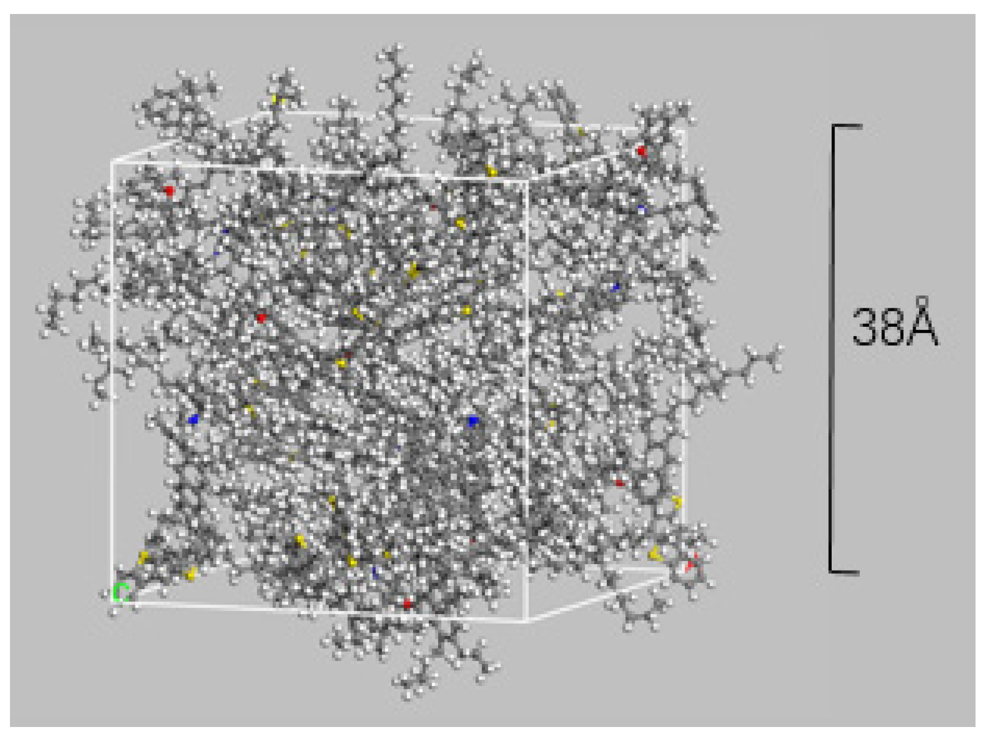
2.1. All-Atom Molecular Model (MD)

Our coarse-grained molecular model is derived from the all-atom MD simulation. In the all-atom MD process, we used the four-components with twelve molecules model of bitumen (

Table 1. Composition of the all-atom molecular model [20].

Molecular Name	Chemical Formula	Number of Molecules Contained in the System
Asphaltene A	C66H81N	3
Asphaltene B	C42H54O	2
Asphaltene C	C51H62S	3
Saturate A	C30H62	4
Saturate B	C35H62	4
Aromatic A	C35H44	11
Aromatic B	C30H46	13
Polar aromatic A	C40H59N	4
Polar aromatic B	C36H57N	4
Polar aromatic C	C18H10S2	15
Polar aromatic D	C40H60S	4
Polar aromatic E	C29H50O	5

) proposed by Li and Greenfield [20], who characterized AAA-1, AAK-1 and AAM-1 studied in the Strategic Highway Research Program (SHRP) by varying the ratio of the number of each type of molecule. This model contains four components: asphaltene, aromatics, saturate and polar aromatic, with N, O and S introduced, which gives a more complete picture of the diversity and complexity of bitumen than the earlier three-component model containing only C and H.

The force field is the basis of MD simulation which, as an approximate treatment of quantum mechanical methods, ignore computationally resource-intensive electronic behavior and can be used for molecular systems with a large number of atoms. There are several suitable force fields for organic matter available for MD simulations of bitumen, such as Universal, Compass, Compass II, OPLS-aa and Gromos96, etc. In our all-atom simulations, the Compass II force field is chosen, which is a molecular force field for studying condensed matter optimization from the atomic level to simulate both organic molecular systems as well as inorganic ones, it is suitable for the simulations of bitumen.

All simulations in this paper were completed using Materials Studio 2017. The all-atom molecular model of bitumen is simulated based on the following steps:

(1)

Twelve different bitumen molecules are drawn and geometrically optimized to eliminate errors in bond lengths, bond angles, etc.;

(2)

Molecules are placed into a computational box with periodic boundary conditions with an initial density of 0.1 g/cm³;

(3)

The system is relaxed for 300 ps in the NVT ensemble, the temperature is set to 298 K. The NVT ensemble refers to a constant temperature, constant volume ensemble where, through NVT relaxation, the bitumen molecules will fully move in the calculation box, thus mixing uniformly and reaching a relatively low energy position, with no change in density during this process;

(4)

It is annealed five times in the temperature range of 263–433 K, which corresponds to the working temperature of road bitumen. Annealing means that the temperature of the system is repeatedly raised and lowered, allowing some of the molecules to break through the energy barrier to reach a less energetic and more stable structure upon return to normal temperature;

(5)

It is simulated for 300 ps in the NPT ensemble, T = 298 K, P = 1 atm. The NPT ensemble refers to a constant temperature and pressure ensemble where the total energy and system volume can be freely varied, and the density of the bitumen system will stabilize through NPT relaxation.

For the control of the NVT and NPT ensembles described above, temperature control and pressure regulation operations are required. We adopt the Berendsen method [21,22], the basic idea of which is to couple the system to a constant temperature external heat bath and to regulate the temperature and pressure of the system by absorbing or releasing energy from the heat bath.

Figure 1 shows the final conformation of the all-atom model (volume = 54.9 nm³) after the above steps, where the colors of the elements C, H, O, N and S are grey, white, red, blue and yellowish, respectively.

Density is the most intuitive parameter of bitumen, indirectly characterizing the static structural properties of the MD model; the diffusion coefficient can be used to represent the rate of movement of the molecules in the bitumen system; bitumen is a polymer, at low temperatures, it appears in a glassy state, with the temperature rising, gradually softening to show viscoelasticity, the glass transition temperature can be used to verify this property of bitumen. The points in the temperature intervals 198–258 K and 268–338 K were fitted linearly, and the horizontal coordinate of the intersection of the two lines is the glass transition temperature of the all-atom molecular model, which is 262.9 K, in addition, bitumen is often used with modifiers, healing agents and other solutions, from the molecular point of view, the solubility parameter characterizes the intermolecular forces of the bitumen. Therefore, density, the diffusion coefficient, glass transition temperature and solubility parameters were chosen to validate the all-atom model.

Table 2. Calculation and reference values of properties of bitumen all-atom molecular model.

Properties	Calculation	Reference Value
Density (g/cm3) (at 288 K)	0.996	1.025 [8]
Diffusion coefficient(cm2/s) (at 298 K)	0.4 × 10−6	0.092 × 10−6 [23]
Glass transition temperature (K)	262.9	261.7 [24]
Solubility parameter (J/cm3)0.5	17.6–18.2	13.3–22.5 [25]

compares the calculated values for the four parameters with reference values from the literature. In general, the calculated values agree well with the reference values.

2.2. Coarse-Grained Model

The core of CGMD is to determine the distribution structure and number of atoms corresponding to a coarse-grained bead, i.e., to determine the mapping scheme. If the number of atoms in the CG bead is too small, the simulation is limited in scale and the calculation efficiency is low. If too many atoms are included, important molecular information (e.g., molecular topology structure and branched chain form) will be lost with insufficient accuracy of the model.

Considering that bitumen molecules are mainly composed of polycyclic aromatic hydrocarbons, unsaturated cyclic aromatic compounds, non-polar hydrocarbons with straight and branched chains and aliphatic cycloalkanes, we considered 16 kinds of coarse beads classified in

Table 3. Beads of bitumen CG molecular model.

Bead Name	Structural Formula	Chemical Formula	Mapping Ratio	Legend	Bead Name	Structural Formula	Chemical Formula	Mapping Ratio	Legend
C3		C3Hn	3		S1		C5HnS	6
C4a		C4Hn	4		B1		C6Hn	6
C4b		C4Hn	4		B2		C4Hn	4
C5a		C5Hn	5		B3		C7Hn	7
C5b		C5Hn	5		B4		C9Hn	9
C6		C6Hn	6		B5		C9HnO	10
N1		C2HnN	3		B6		C6HnS	7
N2		C6HnN	7		B7		C4HnO	5

after repeated calculation. During the division of the coarse-grained beads, the DMol3 module was used to minimize the energy of the functional groups to be coarse-grained, and the GGA-PBE generalization with the DNP group was selected to calculate the optimized structure with the lowest energy. All hydrogen atoms are not abstracted by the structure (including functional groups of hydrogen atoms), and all the chemical formulas on the number of hydrogen atoms are expressed in n, this is due to the fact that the relative atomic mass of hydrogen atoms is small compared with other heavy atoms, besides, the internal forces of the bitumen system are not dominated by hydrogen bonds; the differences in the number of hydrogen atoms within the same CG bead have less influence on the properties of the beads, thus this effect is ignored in this work.

In the model, the coordination ratio of a bead is usually three to seven atoms. C3, C4a, C4b, C5a, C5b, and C6 are hydrocarbon structures without a benzene ring structure, N1, N2, and S1 are non-hydrocarbon structures without a benzene ring structure, B1, B2, B3, B4, B5, B6, and B7 are chemical structures with a benzene ring structure. In order to maintain the integrity of the benzene ring and to preserve as much as possible the characteristics of the benzene functional group, we have done the following special treatment of the benzene ring structure: without splitting the benzene ring structure that exists alone, the relevant structure is mapped as one of the CG beads B1, B4, B5, or B6; for the structure of a compound benzene ring (i.e., structures in which multiple benzene rings share carbon atoms), the mapping is completed with one of B2, B3, or B7 (the red circle in Table 3) attached to B1. For example, naphthalene (C10H8) is mapped as two beads, one B1 and the other B2. Based on the building block approach [26] to build a CG molecule model, the CG structure is kept as all-atoms by the confining effect of the force field. The CG model of all bitumen molecules is shown in Figure 2.

2.3. Coarse-Grained Force Field

The force field determines the motion laws of the simulated system, which is used to describe the inter-particle interactions, including the bonding interaction between particles, the van der Waals force between molecules, the hydrogen bond interaction, the charge force, etc. The basic computational particles of MD are atoms, while CGMD is based on coarse-grained beads, so the all-atom force field is not applicable to the simulation of coarse-grained molecular models.

The CG force field describes all the interaction potential energy functions of coarse-grained beads in the form of potential energy functions, including non-bond potential energy functions and bond potential energy functions:

(1)

The non-bond potential is the energy that mainly affects the determination of macroscopic properties of the bitumen system, including van der Waals potential, hydrogen bond potential and charge energy. Among the non-bonded potential, van der Waals potential plays a major role in the bitumen system. Hydrogen bonds only exist between hydrogen atoms, oxygen atoms, fluorine atoms and nitrogen atoms and must conform to a certain structural general formula; the bitumen molecular model in this study has few oxygen atoms and nitrogen atoms and little influence of hydrogen bonds, so hydrogen bond potential is not considered in this study. The CG beads divided in this study are all neutral particles without charge, so charge energy is not considered in this study.

(2)

The bond potential energy function includes simple harmonic vibration potential energy function, plane bending potential energy function and out-of-plane rocking potential energy function. The bond potential energy plays a minor role in the determination of the macroscopic properties of the bitumen system. In this study, the out-of-plane rocking potential energy function with the least influence on the bitumen system is not considered.

The assumed interaction potential energy is:

$$U_{CG}{=U}_{bond}\left(r\right){+U}_{angle}{\left(\mathsf{\theta }\right)+U}_{non}\left(r\right)$$

(1)

where U_CG is the CG potential, U_bond(r) is the bond energy (assumed harmonic), U_angle(θ) is the angle potential, U_non(r) is the non-bond potential, r is the distance between beads, and θ is the plane angle between three coarse-grained beads.

2.3.1. Non-Bond Potential

Since van der Waals potential energy dominates the bitumen system’s non-bonded potential, the van der Waals force is described as the Lennard–Jones potential [27] in this work. Combined with the “bottom-up” coarse-grained method developed by Voth [28] and Shinoda et al. [29] and starting from the microscopic molecular model, the radial distribution function g(r) is obtained by all-atom simulation of every two coarse beads with van der Waals force. The Boltzmann inversion formula [30] is used to calculate the Lennard–Jones potential function from the radial distribution function, as shown in Formula (2). The Lennard–Jones potential function is provided in Formula (3). It is used to define the non-bonded potential function.

$$U_{non}\left(r\right){=-K}_{B}T\ln \left[g\right(r\left)\right]$$

(2)

where K_B is the Boltzmann constant, T the temperature, and g(r) is the radial distribution function.

This potential is recast into a coarse-grained Lennard–Jones potential

$$U_{LJ}\left(r\right)=4\epsilon \left[{\left(\frac{\sigma }{r}\right)}^{12}-{\left(\frac{\sigma }{r}\right)}^6\right]$$

(3)

where ε and σ are the parameters of the force field. These parameters are estimated by comparing Equation (3) to the all-atom potential: ε corresponds to the lowest energy point of the Lennard–Jones function, while σ to the value of r when the potential is 0.

Table 4. Force field parameter ε.

ε	C3	C4a	C4b	C5a	C5b	C6	B1	B2	B3	B4	B5	B6	B7	N1	N2	S1
C3	0.805	0.806	0.806	0.807	0.806	0.810	0.814	0.806	0.813	0.868	0.882	0.829	0.809	0.608	0.843	0.849
C4a		0.806	0.806	0.807	0.807	0.810	0.815	0.808	0.849	0.869	0.885	0.834	0.811	0.696	0.847	0.855
C4b			0.806	0.807	0.807	0.810	0.815	0.807	0.846	0.870	0.889	0.836	0.812	0.657	0.850	0.856
C5a				0.811	0.811	0.811	0.817	0.809	0.873	0.883	0.907	0.840	0.814	0.762	0.856	0.862
C5b					0.811	0.811	0.817	0.809	0.873	0.885	0.908	0.840	0.815	0.738	0.859	0.861
C6						0.814	0.843	0.812	0.890	0.913	0.948	0.871	0.822	0.781	0.894	0.906
B1							0.962	0.816	0.903	1.014	1.017	0.993	0.838	0.842	0.998	1.007
B2								0.808	0.855	0.842	0.866	0.827	0.817	0.713	0.839	0.840
B3									1.002	0.905	0.929	0.904	0.830	0.746	0.906	0.919
B4										1.036	1.051	0.985	0.856	0.861	1.006	1.028
B5											1.065	1.002	0.882	0.868	1.035	1.042
B6												1.026	0.847	0.849	1.031	1.036
B7													0.823	0.736	1.002	1.014
N1														0.634	0.854	0.857
N2															1.029	1.030
S1																1.034

shows ε, and

Table 5. Force field parameter σ.

σ	C3	C4a	C4b	C5a	C5b	C6	B1	B2	B3	B4	B5	B6	B7	N1	N2	S1
C3	4.80	5.35	5.41	5.47	5.14	5.32	5.39	5.36	5.35	5.68	5.78	5.46	5.377	5.17	5.52	5.55
C4a		5.68	5.88	5.99	5.99	5.73	5.80	5.71	5.69	5.83	5.91	5.82	5.74	5.44	5.83	5.84
C4b			5.79	6.05	6.11	5.85	5.82	5.74	5.81	5.83	5.91	5.82	5.77	5.400	5.83	5.855
C5a				5.95	6.15	5.966	6.03	5.82	5.95	6.05	6.11	6.04	5.87	5.67	6.06	6.08
C5b					6.15	5.97	6.03	5.86	5.94	6.055	6.11	6.055	5.888	5.62	6.044	6.08
C6						5.666	5.77	5.944	5.72	5.84	5.888	5.799	5.91	5.877	5.80	5.81
B1							5.83	5.78	5.78	6.02	6.13	5.88	5.80	5.89	5.966	6.011
B2								5.70	5.744	5.76	5.79	5.77	5.74	5.51	5.77	5.79
B3									5.78	5.85	5.877	5.811	5.85	5.69	5.83	5.83
B4										6.11	6.25	6.02	5.89	5.93	6.05	6.088
B5											6.30	6.08	5.94	5.95	6.12	6.16
B6												5.97	5.88	5.90	5.99	6.02
B7													5.81	5.56	5.90	5.93
N1														5.28	5.78	5.85
N2															6.03	6.044
S1																6.08

shows σ.

2.3.2. Bond Potential

When the CG molecular model is constructed, the non-bond potential function is used to calculate the interaction between beads that are not directly connected, and the bond potential function is used to calculate the interaction between directly connected beads. In the bonding potential function, the simple harmonic vibration potential energy function is expressed as Formula (4), and the plane bending potential energy function is expressed as Formula (5):

The bond coarse-grained potential function is considered harmonic, i.e.,

$$U_{bond}\left(r\right)=\frac{1}{2}{K}_{bond}{\left(r-r_0\right)}^2$$

(4)

$$U_{angle}\left(\theta \right)=\frac{1}{2}{K}_{angle}{\left(cos\mathsf{\theta }-cos{\mathsf{\theta }}_0\right)}^2$$

(5)

K_bond and K_angle are energy constants, r₀ the equilibrium distance between two beads and θ₀ the equilibrium angle among three beads.

In the atomic every two coarse-grained molecular dynamics simulation, beads connected all the all-atom structures of bonding; the tagged two coarse beads had a centroid position in the all-atom structure. The distance between the two coarse beads’ centroids was shown as r₀, as shown in

Table 6. Force field parameter r₀.

r0	C3	C4a	C4b	C5a	B1	B2	B3	B4	B5	B6	B7	N1	N2	S1
C3	4.574	4.629	4.589	4.618	4.683	4.564
C4a		4.686		4.684	4.65	4.593		4.688	4.689
C4b			4.686	4.642	4.711	4.648				4.651			4.757	4.677
C5a				4.516	4.621	4.606	4.659						4.757
C5b					4.589
C6						4.573		4.688						4.677
B1						4.525	4.611			4.689	4.539
B2										4.657		4.619	4.66

. Part of the combination of the two coarse beads did not come linked together by the bitumen molecular model of this study, therefore, there is a blank in Table 6. For the bond angle, the all-atom structure connected by every three coarse-grained beads was simulated, and the position of the centroids of the three coarse-grained beads in the all-atomic structure was marked, and the angle between the lines of the centroids of the three coarse-grained beads was measured as θ₀, as shown in

Table 7. Force field parameter θ₀.

Bead 1	Middle Bead	Bead 2	θ0 (°)	Bead 1	Middle Bead	Bead 2	θ0 (°)
C3	C3	C3	81.6	C3	B1	C4a	154
C3	C3	C4a	84.7	C3	B1	C4b	163.3
C3	C3	C5a	86	C3	B1	C5b	161.5
C3	C3	B1	96.8	C3	B1	B2	165.6
C3	C3	B2	89.3	C3	B1	B3	156.3
C4a	C3	C4a	118.3	C5a	B1	B2	165
C4a	C3	C4b	105.6	C5b	B1	B7	153.1
C4a	C3	B1	107.6	B2	B1	B2	163.4
C4a	C3	B2	100.6	B2	B1	B3	160.3
C4b	C3	C4b	88.5	B2	B1	B7	169.7
C4b	C3	B1	91.3	B6	B1	B6	174.3
C3	C4a	C3	86.3	C3	B2	C3	89.6
C3	C4a	C4a	95.7	C3	B2	C4b	81.6
C3	C4a	B1	86.9	C3	B2	B1	80.9
C3	C4a	B4	86.4	C3	B2	B6	91.6
C3	C4a	N3	83.7	C4a	B2	C5a	89.1
C4a	C4a	C5a	95.3	C4a	B2	B2	89.6
C5a	C4a	B5	162	C4b	B2	B1	74.4
B2	C4a	B2	169.5	C4b	B2	B6	84.8
C3	C4b	C3	167.6	C5a	B2	B1	80
C3	C4b	C4b	170.2	C5a	B2	B6	93.8
C3	C4b	B1	157.3	C5a	B2	N2	85.6
C4b	C4b	C5a	165.5	C6	B2	B1	166.4
C5a	C4b	C5a	144.2	B1	B2	B1	80.5
C5a	C4b	N2	159.5	B1	B2	B2	75.4
C3	C5a	C4b	82.5	B1	B2	B6	85.4
C3	C5a	C5a	75.5	B1	B2	N1	84.6
C4a	C5a	C5a	77.7	C5a	B3	B1	89.9
C4a	C5a	B1	104.9	C4b	B6	B2	152.5
C4b	C5a	C5a	104	B2	B6	B2	153.6
C4b	C5a	B1	97.5	B1	B7	B1	91
C4b	C5a	N2	97.4	C4b	N2	C5a	164
C5a	C5a	C5a	107.6	C4b	N2	B2	162.7
C5a	C5a	N2	108.4	C5a	N2	C5a	161.3
B1	C5a	B2	101.2	C5a	N2	B2	158.2
B4	C6	S1	89.6	C4a	S1	C6	152.7
C3	B1	C3	158.2

. Most combinations of three coarse-grained beads do not form bonding plane angles in the bitumen molecular model in this study, so although 16 different coarse-grained beads can theoretically form 2176 plane Angle combinations, there are only 73 combinations in Table 7. The data in Table 6 and Table 7 are corrected by repeated trial calculation. We use the values of Kbond = 1250 KJ/(mol·nm) and Kangle = 25 KJ/mol. for all bonds and angles, which is consistent with the MARTINI [31].

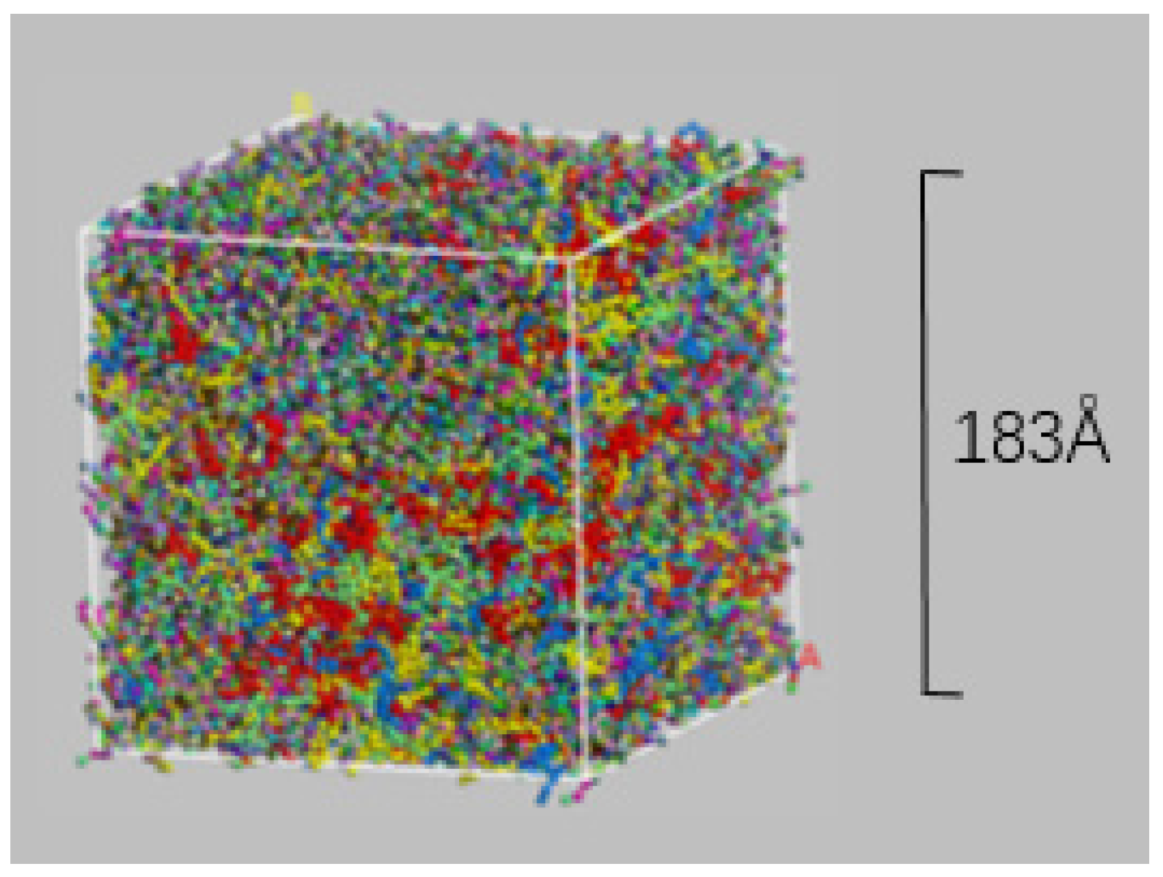
2.4. Coarse-Grained Molecular Dynamics

The equilibration steps for the coarse-grained model are comparable to those of the all-atom one, as follows:

(1)

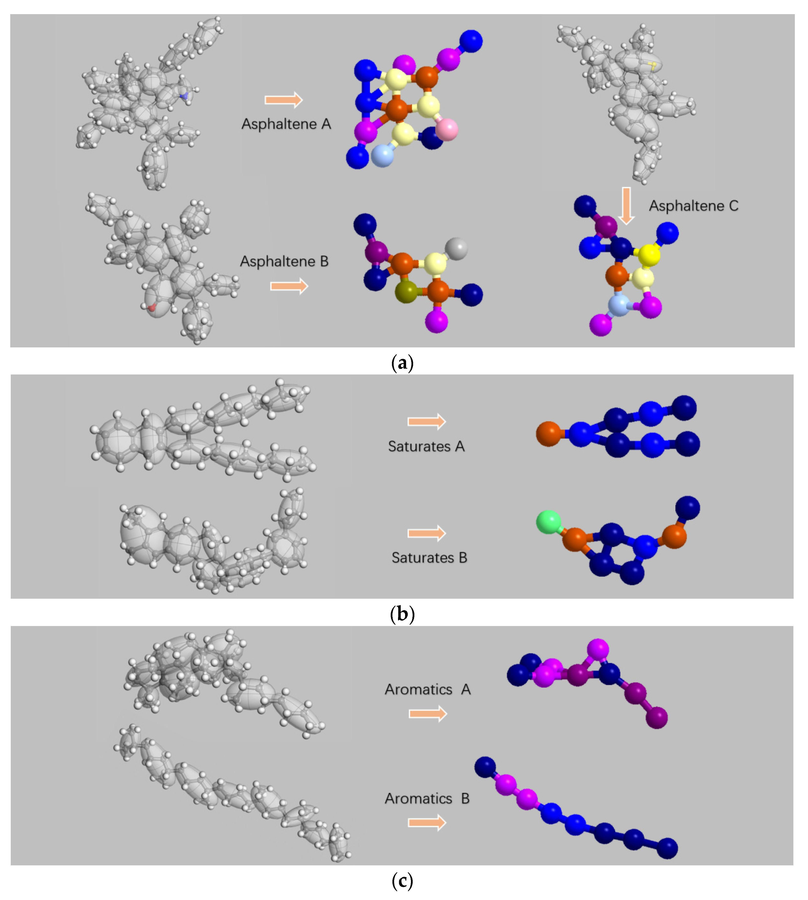
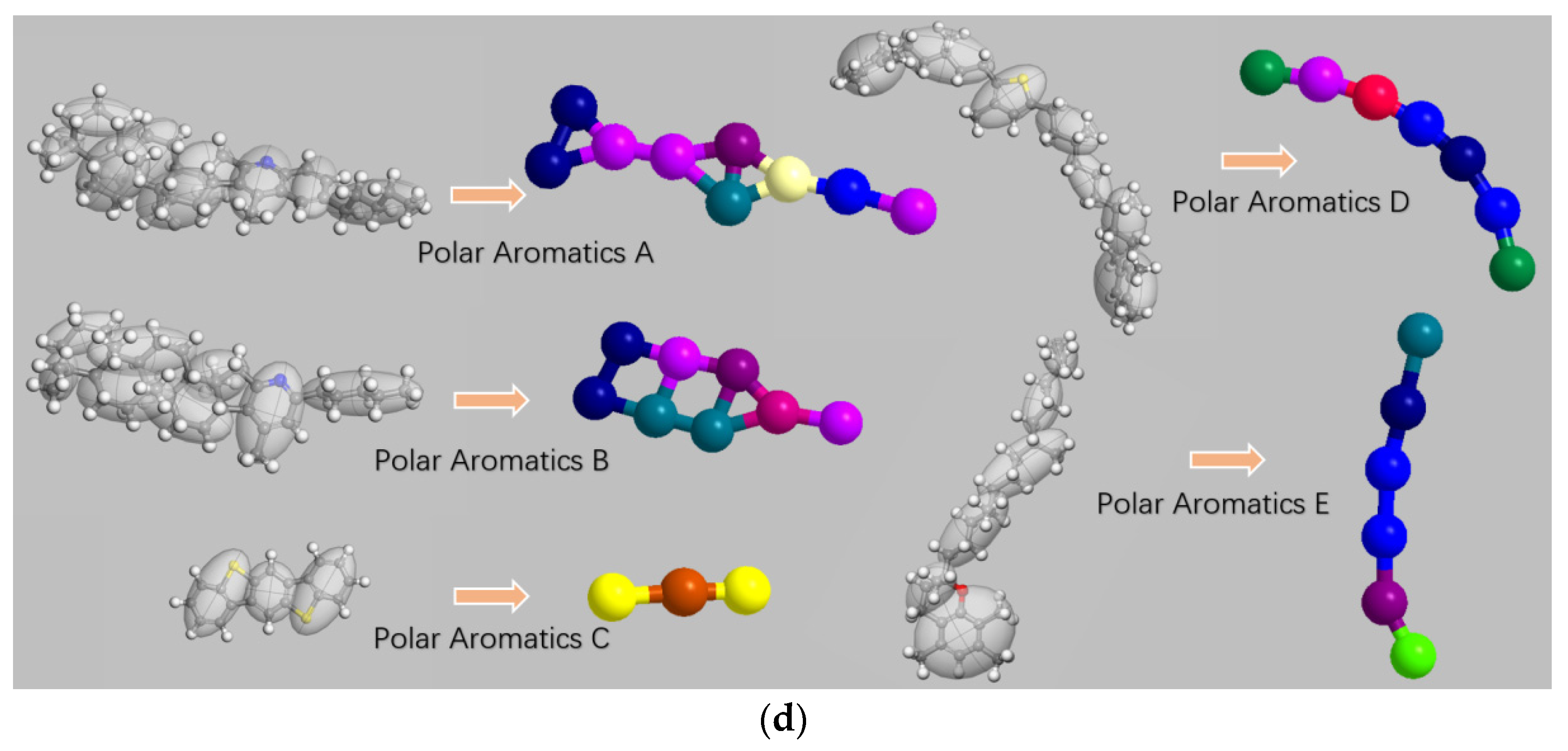
Color the CG molecule models of each component of the bitumen separately for subsequent studies on the effect of the components upon the properties of the bitumen system. The asphaltenes are colored red, the aromatics green, the polar aromatics yellow and the saturates blue.

(2)

Construct a square calculation box with periodic boundary conditions, side lengths of the box are 30 nm and the initial density of the box is 0.15 g/cm³, then input the CG molecular model of each component into the box in terms of the mass ratio;

(3)

Conduct geometric optimization (energy minimization), which should be as full as possible since the CG molecular model is larger with more particles than the all-atom one, setting the number of iterations at 40,000;

(4)

Relaxing the model for 2000 ps at 533 K in the NVT ensemble to reach the energy minimum conformation;

(5)

Simulate the model for 3000 ps at 533 K and 10 atm in the NPT ensemble, then 1000 ps at 1 atm. The 10 atm run is for accelerating the compression of the model, and the 1atm run is to achieve the desired final pressure.

The final configuration is shown in Figure 3. The volume of the simulation is 6128.5 nm³, which is about 112 times that of the all-atom molecular model.

2.5. Validation of the Bitumen CG Molecular Model

Similar to the validation method of the all-atom molecular model, density, diffusion coefficient and molecular aggregation behavior were chosen as metrics to validate the CG molecular model.

The average density of the model is 0.878 g/cm³ at 10 standard atmospheric pressures, T = 533 K, while at 1 standard atmospheric pressure, T = 533 K, the average density is 0.876 g/cm³. The small difference in density between atmospheric pressures indicates a stable system. The density of the model at 1 standard atmospheric pressure, T = 288 K is 1.023 g/cm³, which is close to the reference 1.025 g/cm³ in Table 2.

Simulating the CG molecular model at a temperature of 298 K for 200 ps in an NPT ensemble, the diffusion coefficient was calculated to be 2.522 × 10⁻⁶ cm²/s, which is close to 3.5 × 10⁻⁶ cm²/s measured by Andrews et al. [32] using fluorescence correlation spectroscopy.

The change in the trajectory of the CG molecules is shown in Figure 4, where the molecules exhibit molecular aggregation behavior in the NVT ensemble simulation, forming agglomerates and further forming nanoaggregates [33].

Based on the above validation, the CG bitumen molecular model is considered reasonable and can be used for further research.

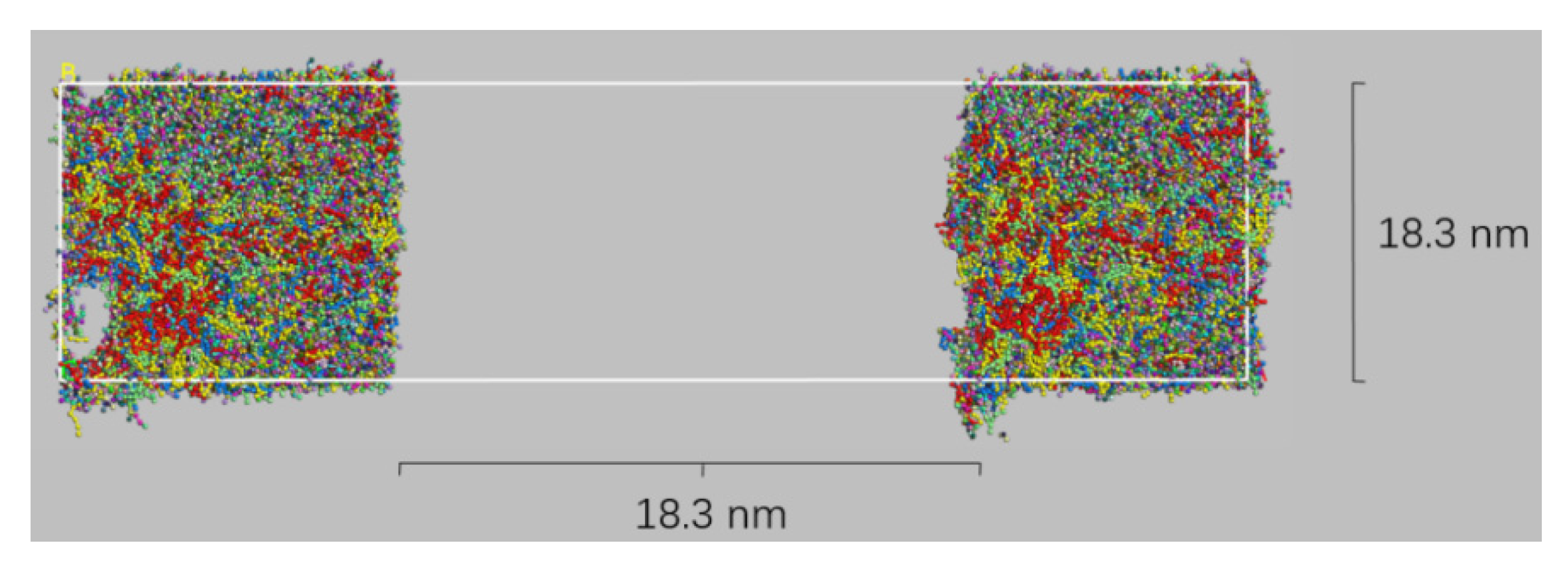
2.6. Bitumen Healing

The calculation box’s dimensions for the microcrack simulations are 73.2 nm in length and 18.3 nm in height. The CG molecular model in Figure 3 is placed on both sides of the box to represent the bitumen before healing. The microcrack is represented by the empty area in the center of the box. The system is geometrically optimized for 50,000 iterations. The obtained bitumen microcrack model is shown in Figure 5. The volume of microcracks in this model is approximately 481 times that of all-atoms microcracks [8], and the microcrack width (36.6 nm) is about 18 times larger, which will be helpful to study the self-healing behavior and other mesoscopic properties of bitumen on a larger scale.

NPT ensemble simulations of bitumen microcrack models were carried out at 273, 283, 293, 303, 313, 323, 333, 343, 353, 363 and 373 K for 500 ps.

3. Results and Discussion

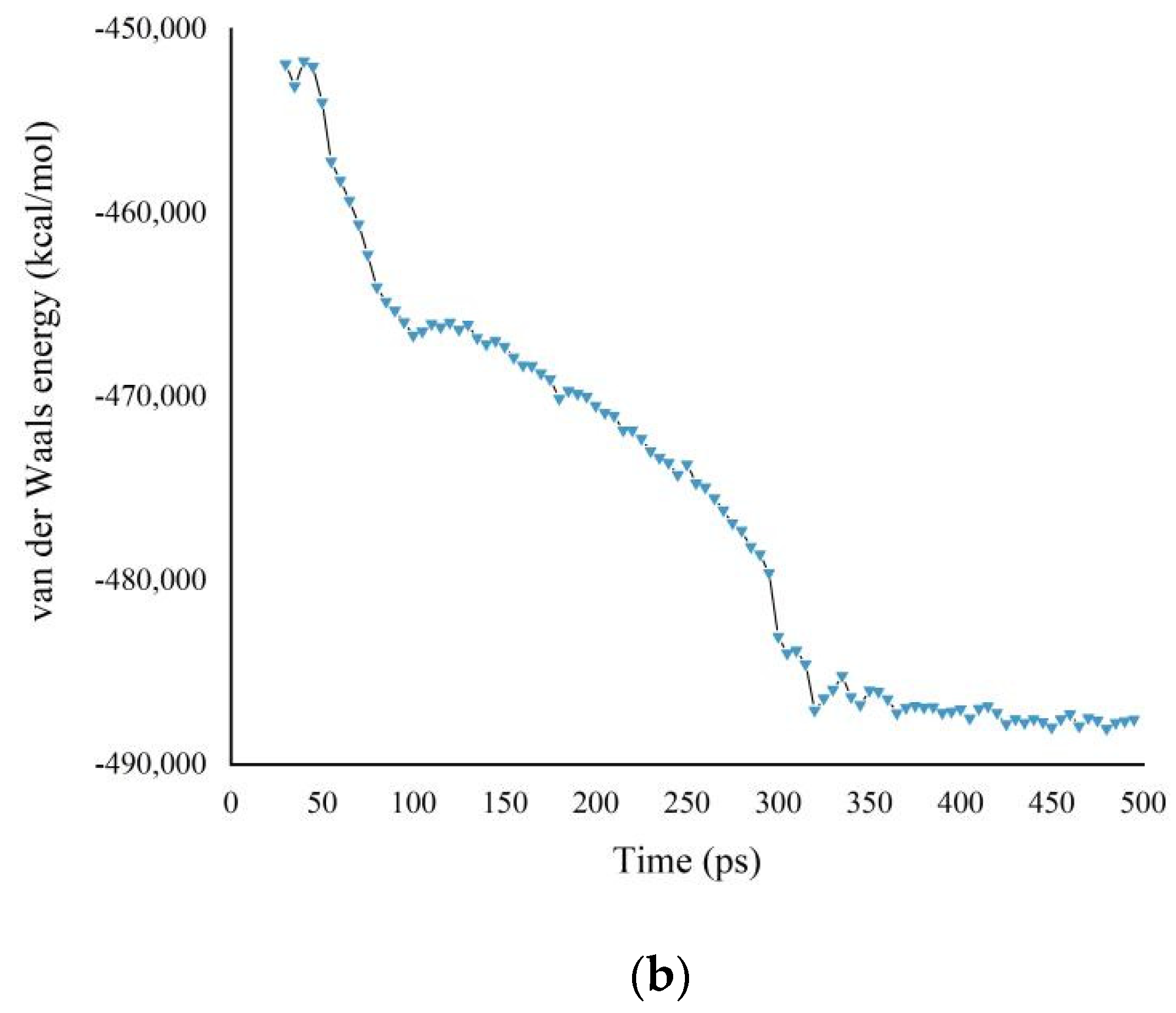
3.1. Potential Energy

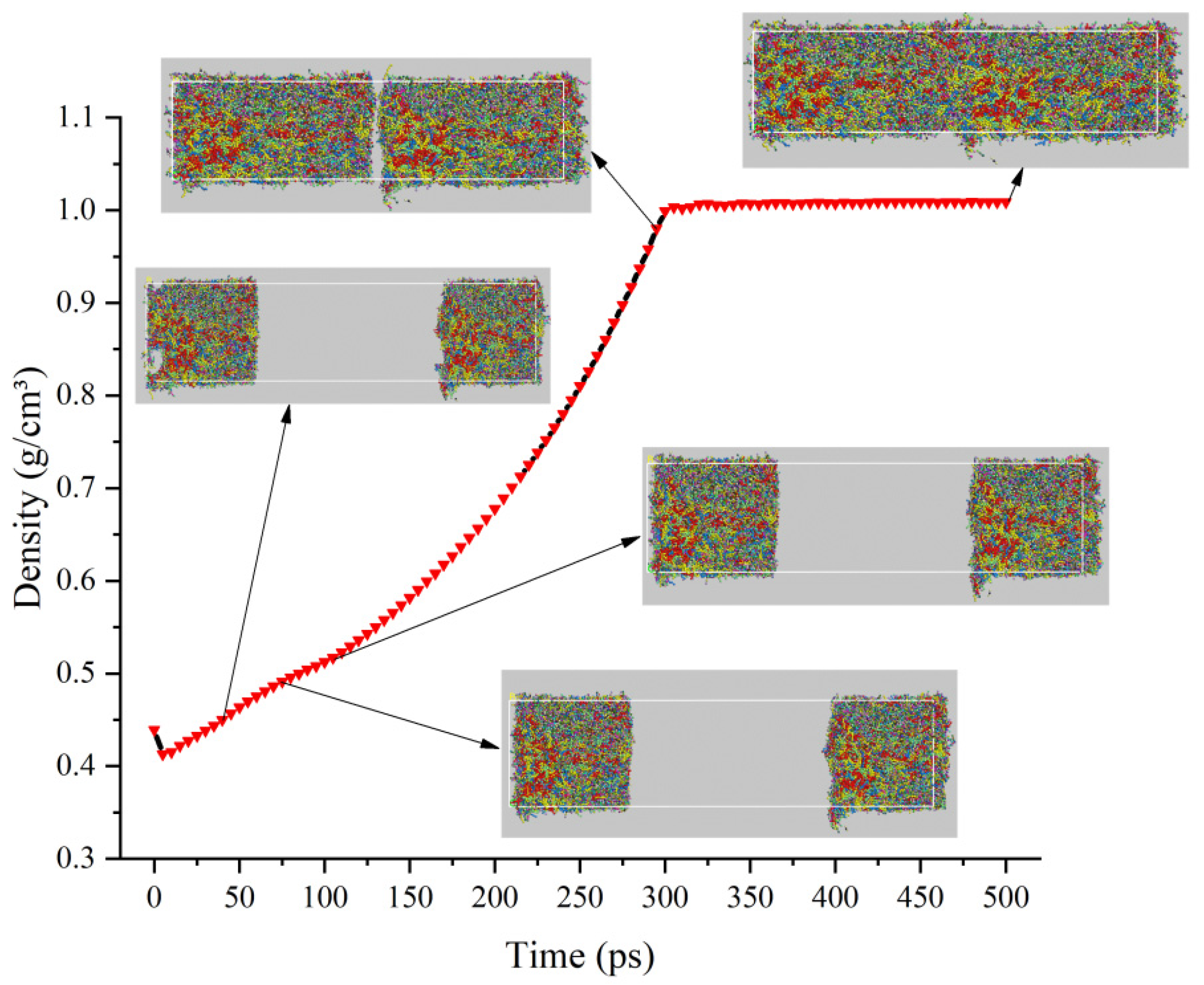
Figure 6 depicts the energy development of the system at 333 K during the healing procedure. At around 300 ps, the microcrack’s two sides come into contact.

The bond energy remains constant while the other two components diminish as the two sides of the crack get closer to one another. This situation indicates that the healing-driven forces at the molecular level are the angle and van der Walls forces, but not the bond energy. The molecules do not stretch to fill the empty space but ‘unfold’ assuming a straighter shape, while the two sides are attracted to each other by van der Walls forces. After the two sides touch, the van der Walls attraction presses one side against the other, compressing the molecules and increasing the bond potential. This evolution is interesting because it shows that during healing, the molecular structure of bitumen changes. Therefore, even if the bitumen may appear the same under a microscope, there is a clear difference before and after healing.

3.2. Density

The change in density of the system reflects the healing of asphalt over time. The density of the box calculated during the simulation at 333 K is shown in Figure 7.

As healing progresses, density increases (the total mass is constant, but the volume changes due to the NPT ensemble). The density of model healing was about 1.002 g/cm³. The density close to the CG molecular model of bitumen is 1.023 g/cm³.

The density slows down the rising rate at about 80 ps after the start of the simulation and accelerates the rising rate at about 110 ps after the simulation initiates, which is consistent with the changing trend of the length, width, and height curve of the calculated box. The overall form of bitumen fluctuates dramatically in the first 80 ps and thereafter, stabilizes in accordance with the molecular motion trajectory. It is speculated that the bitumen molecular motion is mainly self-balancing and internal molecular recombination before the 80 ps. Until the crack is repaired as a result of molecular diffusion motion, the molecular motion is largely a diffusion motion starting at 80 ps and reaching its peak rate of diffusion motion at 110 ps.

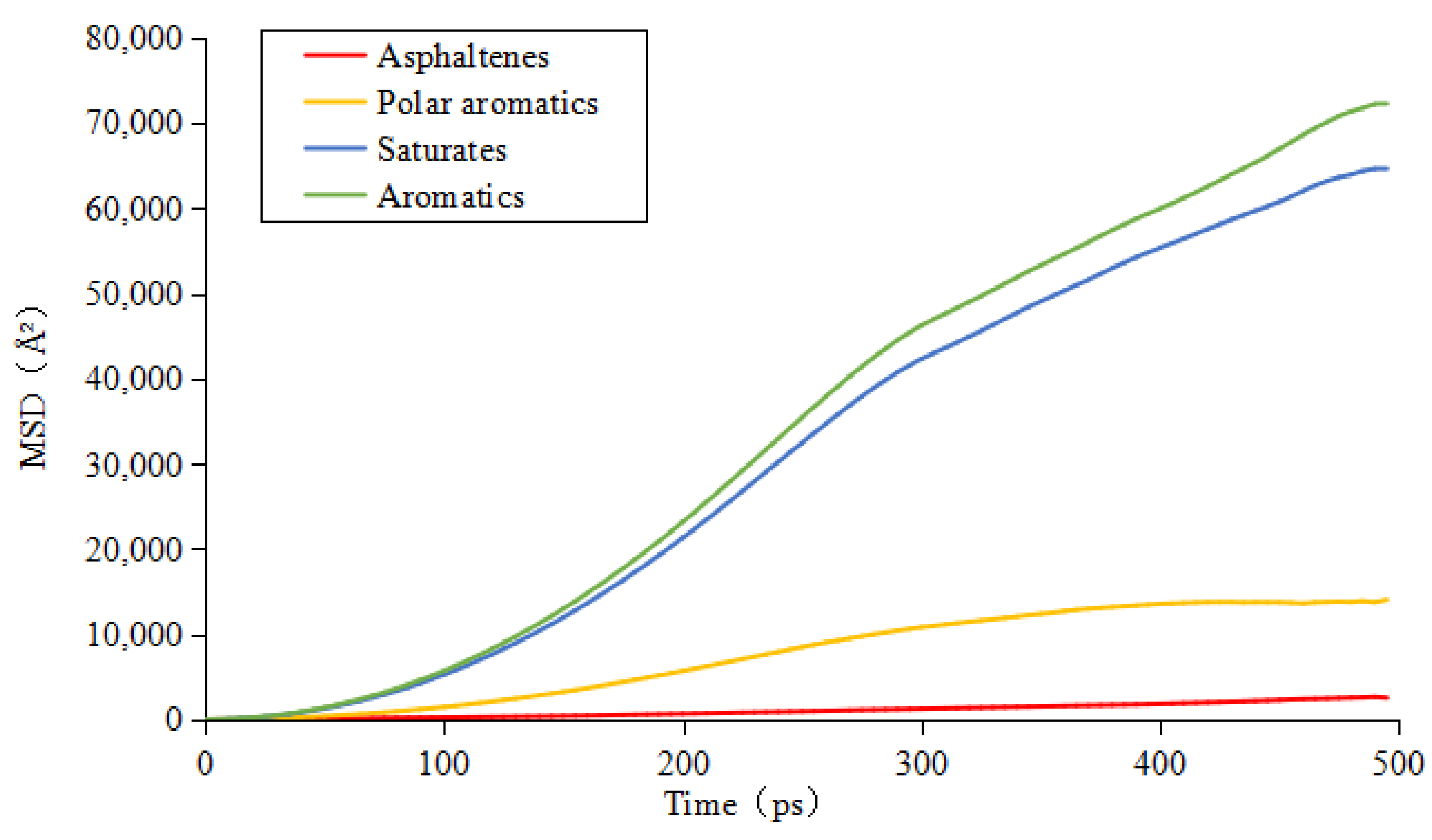
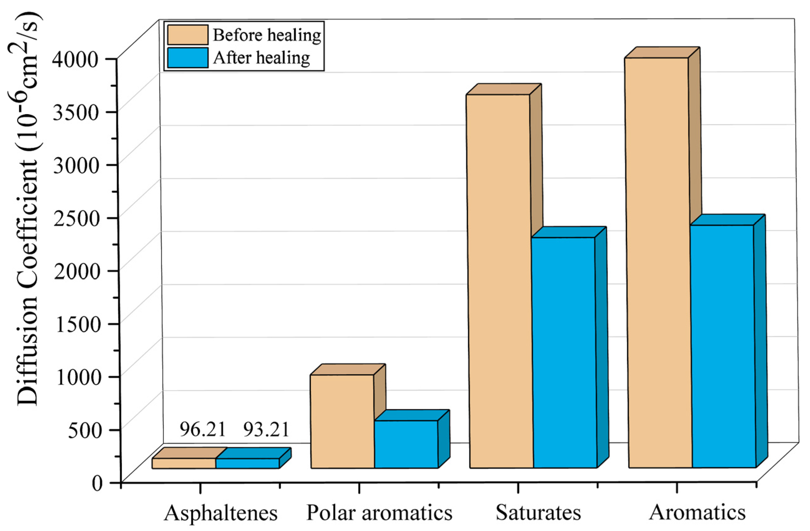
3.3. Diffusion Coefficient

From the microscopic perspective, the speed of molecular motion can be represented by the diffusion coefficient, and there is a certain relationship between the mean square displacement (MSD) and the diffusion coefficient [34]. Theoretically, if the time is long enough, the slope of the function of lg (MSD) and lg (Time) should be 1, at which time Einstein diffusion occurs, and the self-diffusion coefficient of bitumen component can be calculated only when this condition is met [35]. However, due to the short simulation time of molecular dynamics, as long as the function of MSD and time is linear, the diffusion coefficient can be calculated by the slope.

The healing time is about 300 ps. For each component, we can calculate the slope of the MSD versus time function in the range of 150–295 ps and 300–410 ps (in these two time periods, the function of MSD and time is almost linear, which is shown in Figure 8) and convert them into the diffusion coefficient of each component molecule before and after healing. The diffusion rate of each component is asphaltenes < polar aromatics < saturates < aromatics. The diffusion rate of saturates is relatively close to that of aromatics, which is much greater than that of asphaltenes and polar aromatics. This phenomenon is consistent with colloidal theory [33]. According to this theory, asphaltene, which is at the core of the colloidal bitumen system, should have the lowest diffusivity. Saturates and aromatics, on the other hand, are in the shell and should have higher diffusivity.

The diffusion coefficients of the four components decrease during healing. As shown in Figure 9, asphaltenes decreased by about 3.1%, polar aromatics by roughly 49.0%, saturates decreased by about 38.3%, and aromatics decreased by about 40.8%. The reason why the healing affects the bitumen molecular diffusion coefficient is that, as bitumen heals, the free movement space of bitumen molecules becomes less and less. This effect is more significant on polar aromatics, saturates, and aromatics. This indicates that the self-healing behavior of bitumen is the main reason for the molecular diffusion of the polar aromatics, saturates fraction, and aromatics fraction, while the self-healing behavior of bitumen hardly affects the molecular diffusion of asphaltenes. Saturates and aromatics appear to be the primary contributors to the self-healing behavior of bitumen since their diffusion coefficients are substantially greater than those of asphaltenes and polar aromatics.

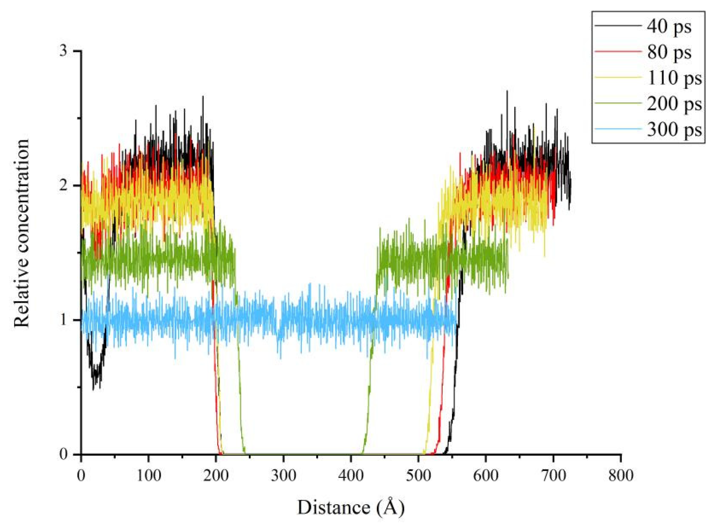
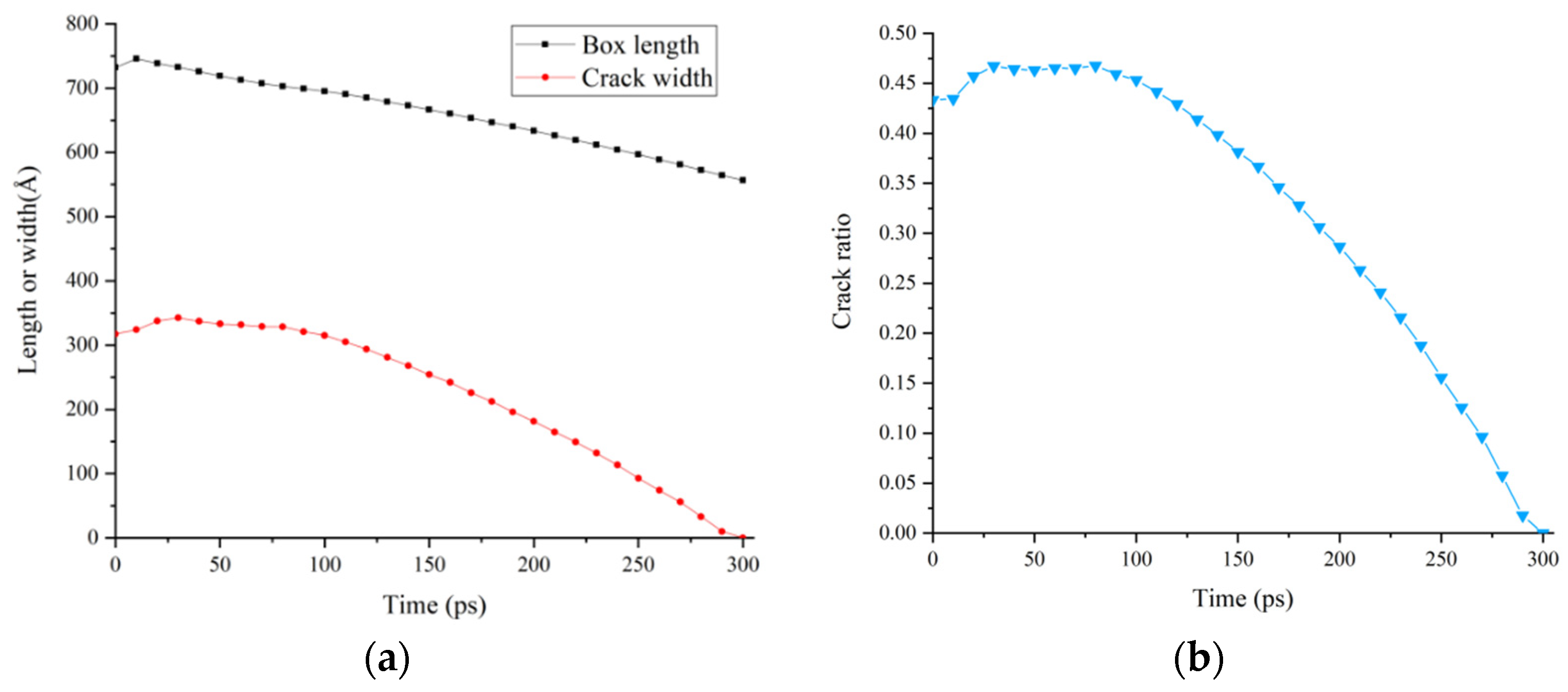
3.4. Relative Concentration and Crack Ratio

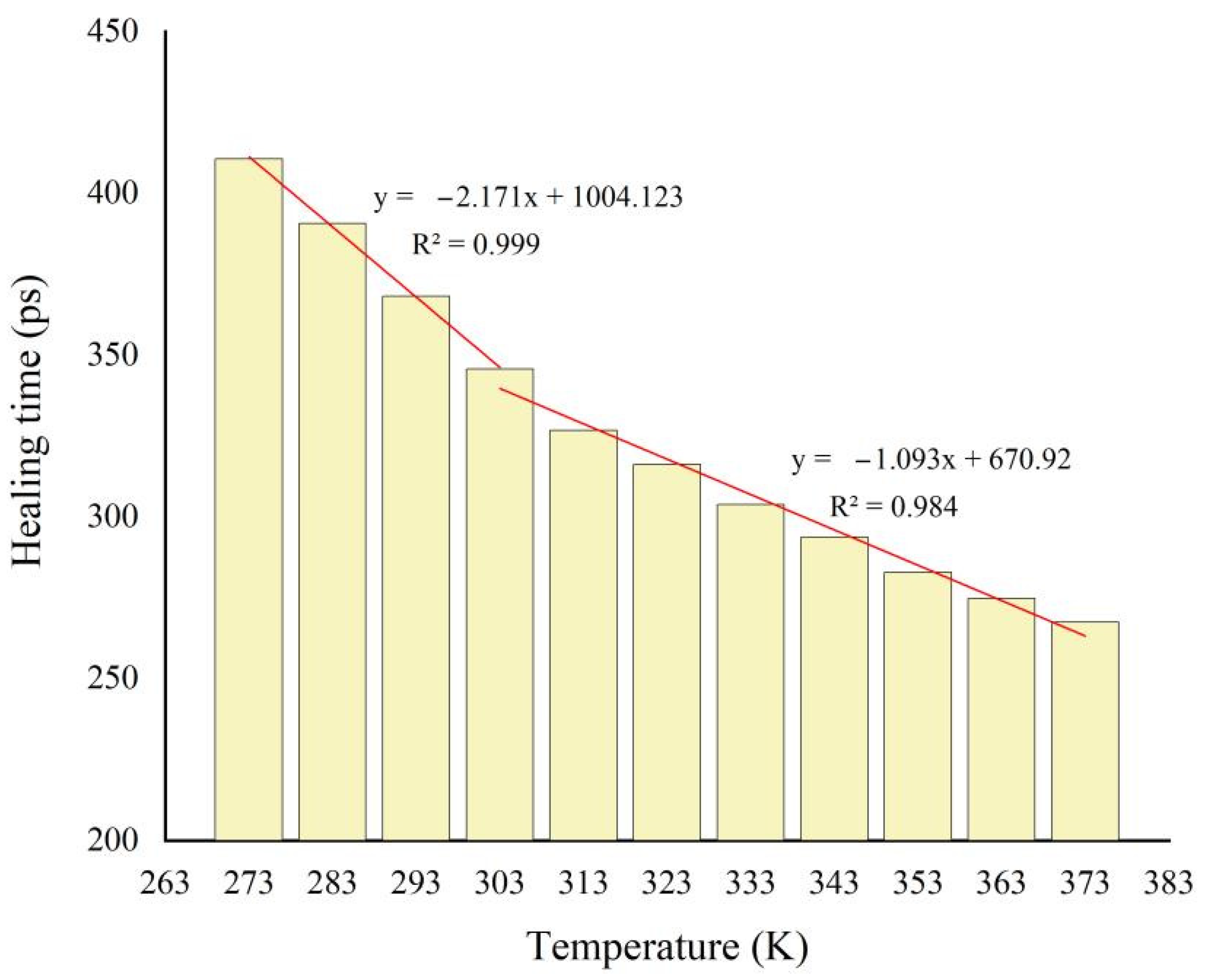
The relative concentration represents the fraction of molecules in a given direction. For a 3D box with XYZ coordinates, the analysis of relative concentration is more like a slice of the box. The larger the relative concentration at a point in the Z direction, the more molecules in the XY slice at this point. The relative concentration of molecules will be close to 0 at the position where voids completely appear in the box. The relative concentration can be calculated as:

$$\mathit{RC}=\frac{n_s/V_s}{n/V}$$

(6)

Among them, RC is the relative concentration of molecules, n_s is the number of particles in a cross-section perpendicular to the coordinate axis in the box, V_s is the volume of the cross-section, n is the number of particles in the calculated box, and V is the volume of the calculated box.

Taking 333 K as an example, the relative concentration of molecules along the length of the box in the simulation process of the model is shown in Figure 10. Among them, 40 ps roughly corresponds to the moment the model achieves initial self-balance, 80 ps roughly corresponds to the moment the bitumen’s overall shape changes, 110 ps roughly corresponds to the moment the model’s healing rate starts to accelerate, and 300 ps roughly corresponds to the moment the model achieves healing.

The change in relative concentration is consistent with the molecular trajectory. As the simulation progresses, the crack in the center of the model becomes narrower, and the interval with the value of 0 in the center of the relative concentration diagram becomes shorter. The box’s length steadily reduces as a result of the NPT ensemble simulation, and the relative concentration broken line diagram gradually gets shorter. As the bitumen at both ends of the model gradually moves towards the central crack, the relative concentration of bitumen molecules at both ends gradually decreases.

For the relative concentration along the length direction at a specific time, the maximum value of the abscissa represents the box length at that time, and the length of the interval with the value of 0 in the center represents the crack width at that time. Due to the NPT ensemble simulation, the box shrinks with the simulation, and the crack width is the result of the reduction in the box length, which cannot directly represent the degree of crack healing. Therefore, the parameter crack rate is defined in this paper to characterize the degree of crack healing.

$$c=\frac{w}{l}$$

(7)

Among them, c is the crack rate at a certain time, w is the crack width at that time, and l is the box length at that time.

Taking 333 K as an example, the crack width, box length, and corresponding crack rate of the model before healing are shown in Figure 11.

The model enters a state of self-balancing during the first 40 ps, during which time, the box length, crack width, and crack rate all increase. The box length essentially maintains a constant rate of reduction after 40 ps, which is in line with the features of NPT ensemble simulation. The crack width basically maintained a constant rate of decline within the 40–80 ps, accelerated from the 80 ps, slowed down at about 290 ps, and decreased to 0 at about 300 ps. The crack rate remained basically unchanged in the 40ps to 80 ps, accelerated from the 80 ps, slowed down at about 290 ps, and decreased to 0 at about 300 ps.

According to the molecular trajectory, 80 ps is the time when the model completes the internal molecular reorganization, and 290 ps is the time when the bitumen molecules at both ends of the model begin to contact. The above analysis of the crack rate shows that at the initial stage of the self-healing behavior of bitumen, the bitumen molecules undergo internal molecular reorganization, and the cracks almost do not heal at this time; after internal molecular recombination, bitumen cracks begin to heal, and the healing rate continues to rise; when the bitumen molecules at both ends of the crack begin to contact, the crack healing rate decreases until the completion of healing.

3.5. Temperature

Figure 12 displays the model’s healing time at various temperatures. The molecular diffusion process is more vigorous and heals more quickly at higher temperatures. As a result, the relationship between temperature and crack healing time is inverse. According to the slope in Figure 12, when the temperature is lower than 303 K, the effect of temperature is more pronounced. A possible explanation of this behavior is that 303 K is close to the glass transition temperature of bitumen, and an increase in temperature has a higher effect on molecular diffusion if the material is in the glass phase.

4. Conclusions

In this work, the CG model was established based on the data of the MD simulation of bitumen, the force field parameters were calculated, and the coarse-grained force field suitable for the CG molecular model of bitumen was developed and verified. At the same time, the model was used in the study of self-healing bitumen. The main research conclusions are as follows:

According to the structure characteristics of the four-component bitumen model with twelve molecules, 16 mapping schemes of CG beads were divided; the integrity of the benzene ring functional groups was preserved as far as possible, while the thickened benzene ring structure was mapped by using two CG beads connected to each other. The Boltzmann inversion was used to calculate the non-bond potential energy, and the harmonic potential was used to calculate the bond potential energy to obtain the force field parameters. Compared with the all-atom model, the CG model has a longer simulation time and larger scale, which will be helpful in studying the self-healing behavior of healing agent-doped and aged asphalt at the mesoscopic scale.

By studying CG models of microcracks in bitumen, it was found at the molecular level that angle and van der Waals forces are the driving forces for self-healing; the molecules “unfold” into a straighter shape as the van der Waals forces pull the two sides of the crack together, rather than stretching to fill the vacant. The variation in cracking rate showed that increasing the temperature near the glass transition temperature of bitumen accelerates the molecular diffusion movement more significantly. At the same time, the diffusivity of saturates, aromatics decreased greatly during the healing process, proving that the components mainly contributing to the self-healing behavior of bitumen are the saturates and aromatics.

References

1. Zhang, L.; Greenfield, M.L. Molecular Orientation in Model Asphalts Using Molecular Simulation. Energy Fuels 2007, 21, 1102–1111. [Google Scholar] [CrossRef]
2. Li, D.D.; Greenfield, M.L. Chemical compositions of improved model asphalt systems for molecular simulations. Fuel 2014, 115, 347–356. [Google Scholar] [CrossRef]
3. Li, D.D.; Greenfield, M.L. Viscosity, relaxation time, and dynamics within a model asphalt of larger molecules. J. Chem. Phys. 2014, 140, 034507. [Google Scholar] [CrossRef] [PubMed]
4. Shen, S.; Lu, X.; Liu, L.; Zhang, C. Investigation of the influence of crack width on healing properties of asphalt binders at multi-scale levels. Constr. Build. Mater. 2016, 126, 197–205. [Google Scholar] [CrossRef]
5. Sun, D.; Sun, G.; Zhu, X.; Ye, F.; Xu, J. Intrinsic temperature sensitive self-healing character of asphalt binders based on molecular dynamics simulations. Fuel 2018, 211, 609–620. [Google Scholar] [CrossRef]
6. Qu, X.; Wang, D.; Hou, Y.; Liu, Q.; Oeser, M.; Wang, L. Investigation on Self-Healing Behavior of Asphalt Binder Using a Six-Fraction Molecular Model. J. Mater. Civ. Eng. 2019, 31, 04019046. [Google Scholar] [CrossRef]
7. He, L.; Li, G.; Lv, S.; Gao, J.; Kowalski, K.J.; Valentin, J.; Alexiadis, A. Self-healing behavior of asphalt system based on molecular dynamics simulation. Constr. Build. Mater. 2020, 254, 119225. [Google Scholar] [CrossRef]
8. He, L.; Zheng, Y.; Alexiadis, A.; Cannone Falchetto, A.; Li, G.; Valentin, J.; Van den bergh, W.; Emmanuilovich Vasiliev, Y.; Kowalski, K.J.; Grenfell, J. Research on the self-healing behavior of asphalt mixed with healing agents based on molecular dynamics method. Constr. Build. Mater. 2021, 295, 123430. [Google Scholar] [CrossRef]
9. Sun, W.; Wang, H. Self-healing of asphalt binder with cohesive failure: Insights from molecular dynamics simulation. Constr. Build. Mater. 2020, 262, 120538. [Google Scholar] [CrossRef]
10. Hu, D.; Pei, J.; Li, R.; Zhang, J.; Jia, Y.; Fan, Z. Using thermodynamic parameters to study self-healing and interface properties of crumb rubber modified asphalt based on molecular dynamics simulation. Front. Struct. Civ. Eng. 2020, 14, 109–122. [Google Scholar] [CrossRef]
11. Gong, Y.; Xu, J.; Yan, E.; Cai, J. The Self-Healing Performance of Carbon-Based Nanomaterials Modified Asphalt Binders Based on Molecular Dynamics Simulations. Front. Mater. 2021, 7, 599551. [Google Scholar] [CrossRef]
12. Zhang, X.; Zhou, X.; Zhang, F.; Ji, W.; Otto, F. Study of the self-healing properties of aged asphalt-binder regenerated using residual soybean-oil. J. Appl. Polym. Sci. 2022, 139, 51523. [Google Scholar] [CrossRef]
13. Tripathy, M.; Agarwal, U.; Kumar, P.B.S. Toward Transferable Coarse-Grained Potentials for Poly-Aromatic Hydrocarbons: A Force Matching Approach. Macromol. Theory Simul. 2018, 28, 1800040. [Google Scholar] [CrossRef] [Green Version]
14. Mohammadi, K.; Madadi, A.A.; Bajalan, Z.; Pishkenari, H.N. Analysis of mechanical and thermal properties of carbon and silicon nanomaterials using a coarse-grained molecular dynamics method. Int. J. Mech. Sci. 2020, 187, 106112. [Google Scholar] [CrossRef]
15. Eichenberger, A.P.; Huang, W.; Riniker, S.; van Gunsteren, W.F. Supra-Atomic Coarse-Grained GROMOS Force Field for Aliphatic Hydrocarbons in the Liquid Phase. J. Chem. Theory Comput. 2015, 11, 2925–2937. [Google Scholar] [CrossRef] [PubMed]
16. Yaxin, A.; Bejagam, K.K.; Deshmukh, S.A. Development of New Transferable Coarse-Grained Models of Hydrocarbons. J. Phys. Chem. B 2018, 122, 7143–7153. [Google Scholar]
17. Garrido, J.M.; Cartes, M.; Mejía, A. Coarse-grained theoretical modeling and molecular simulations of nitrogen + n -alkanes: ( n -pentane, n -hexane, n -heptane, n -octane). J. Supercrit. Fluids 2017, 129, 83–90. [Google Scholar] [CrossRef]
18. Jiménez-Serratos, G.; Totton, T.S.; Jackson, G.; Müller, E.A. Aggregation Behavior of Model Asphaltenes Revealed from Large-Scale Coarse-Grained Molecular Simulations. J. Phys. Chem. B 2019, 123, 2380–2396. [Google Scholar] [CrossRef]
19. Li, G.; Han, M.; Tan, Y.; Meng, A.; Li, J.; Li, S. Research on bitumen molecule aggregation based on coarse-grained molecular dynamics. Constr. Build. Mater. 2020, 263, 120933. [Google Scholar] [CrossRef]
20. Li, L.; Zhang, N.; Sun, D. Road Engineering Materials; China Communication Press: Beijing, China, 2011. [Google Scholar]
21. Berendsen, H.J.C.; Postma, J.P.M.; van Gunsteren, W.F.; DiNola, A.; Haak, J.R. Molecular dynamics with coupling to an external bath. J. Chem. Phys. 1984, 81, 3684–3690. [Google Scholar] [CrossRef] [Green Version]
22. Hoover, W.G. Canonical dynamics: Equilibrium phase-space distributions. Phys. Rev. A Gen. Phys. 1985, 31, 1695. [Google Scholar] [CrossRef] [PubMed]
23. Xu, G.J. Characterization of Asphalt Properties and Asphalt-Aggregate Interaction Using Molecular Dynamics Simulation. Ph.D. Thesis, Rutgers University Community Repository, Rutgers, NJ, USA, 2017. [Google Scholar]
24. Robertson, R.E.; Branthaver, J.F.; Harnsberger, P.M.; Peterson, J.C.; Dorrence, S.M.; Mckay, J.F.; Turner, T.F.; Pauli, A.T.; Huang, S.C.; Huh, J.D. Fundamental Properties of Asphalt and Modified Asphalts; Western Research Institute: Laramie, WY, USA, 2001; Volume I. [Google Scholar]
25. Xu, G.; Wang, H. Study of cohesion and adhesion properties of asphalt concrete with molecular dynamics simulation. Comput. Mater. Sci. 2016, 112, 161–169. [Google Scholar] [CrossRef]
26. Voth, G.A. On the Development of Coarse-Grained Protein Models. In Coarse-Graining of Condensed Phase and Biomolecular Systems; CRC Press: Boca Raton, FL, USA, 2008; pp. 141–156. [Google Scholar]
27. Youngs, T.G.A.; Del Pópolo, M.G.; Kohanoff, J. Development of complex classical force fields through force matching to ab initio data: Application to a room-temperature ionic liquid. J. Phys. Chem. B 2006, 110, 5697–5707. [Google Scholar] [CrossRef] [PubMed]
28. Voth, G.A. Coarse-Graining of Condensed Phase and Biomolecular Systems; CRC Press: Boca Raton, FL, USA, 2009. [Google Scholar]
29. Shinoda, W.; Delvane, R.; Klein, M.L. Multi-property fitting and parameterization of a coarse grained model for aqueous surfactants. Mol. Simul. 2007, 33, 27–36. [Google Scholar] [CrossRef]
30. Lyubartsev, A.P.; York, R.; Heald, E.F. Modeling a Boltzmann Distribution: Simbo (Simulated Boltzmann). J. Chem. Educ. 2003, 80, 109. [Google Scholar] [CrossRef]
31. Marrink, S.J.; Risselada, H.J.; Yefimov, S.; Tieleman, D.P.; de Vries, A.H. The MARTINI Force Field: Coarse Grained Model for Biomolecular Simulations. J. Phys. Chem. B 2007, 111, 7812–7824. [Google Scholar] [CrossRef] [Green Version]
32. Andrews, A.; Guerra, R.; Mullins, O.; Sen, P. Diffusivity of Asphaltene Molecules by Fluorescence Correlation Spectroscopy. J. Phys. Chem. A 2006, 110, 8093–8097. [Google Scholar] [CrossRef]
33. Mullins, O.C. The Modified Yen Model. Energy Fuels 2010, 24, 2179–2207. [Google Scholar] [CrossRef]
34. Wu, G.; He, L.; Chen, D. Sorption and Distribution of Asphaltene, Resin, Aromatic and Saturate Fractions of Heavy Crude Oil on Quartz Surface: Molecular Dynamic Simulation. Chemosphere 2013, 92, 1465–1471. [Google Scholar] [CrossRef]
35. Einstein, A. On the Movement of Small Particles Suspended in Stationary Liquids Required by the Molecular-Kinetic Theory of Heat. Ann. Phys. 1905, 17, 549–560. [Google Scholar] [CrossRef]
Figure 1. All-atom molecular model of bitumen.
Applsci 12 10360 g001
Figure 2. The mapping scheme of the bitumen molecule model. (a) Mapping scheme of asphaltenes. (b) Mapping scheme of saturates. (c) Mapping scheme of aromatics. (d) Mapping scheme of polar aromatics.
Applsci 12 10360 g002aApplsci 12 10360 g002b
Figure 3. Coarse-grained molecular model of bitumen.
Applsci 12 10360 g003
Figure 4. Molecular trajectories of bitumen CG systems at NVT ensemble. (a) 500 ps; (b) 1500 ps; (c) 2000 ps.
Applsci 12 10360 g004
Figure 5. Bitumen microcrack model.
Applsci 12 10360 g005
Figure 6. Potential energy of model in the self-healing process. (a) Bond energy and angle energy; (b) van der Waals energy.
Applsci 12 10360 g006aApplsci 12 10360 g006b
Figure 7. The density of the model in the process of self-healing.
Applsci 12 10360 g007
Figure 8. MSD of each component.
Applsci 12 10360 g008
Figure 9. Diffusion coefficient of each component before and after healing.
Applsci 12 10360 g009
Figure 10. Relative concentration at each time during the self-healing process of the model.
Applsci 12 10360 g010
Figure 11. Healing degree parameters of the model in the process of self-healing. (a) Crack width and box length; (b) Crack ratio.
Applsci 12 10360 g011
Figure 12. Healing time of microcrack model.
Applsci 12 10360 g012