
An Optimization of Statistical Index Method Based on Gaussian Process Regression and GeoDetector, for Higher Accurate Landslide Susceptibility Modeling


Abstract
1. Introduction
2. Materials
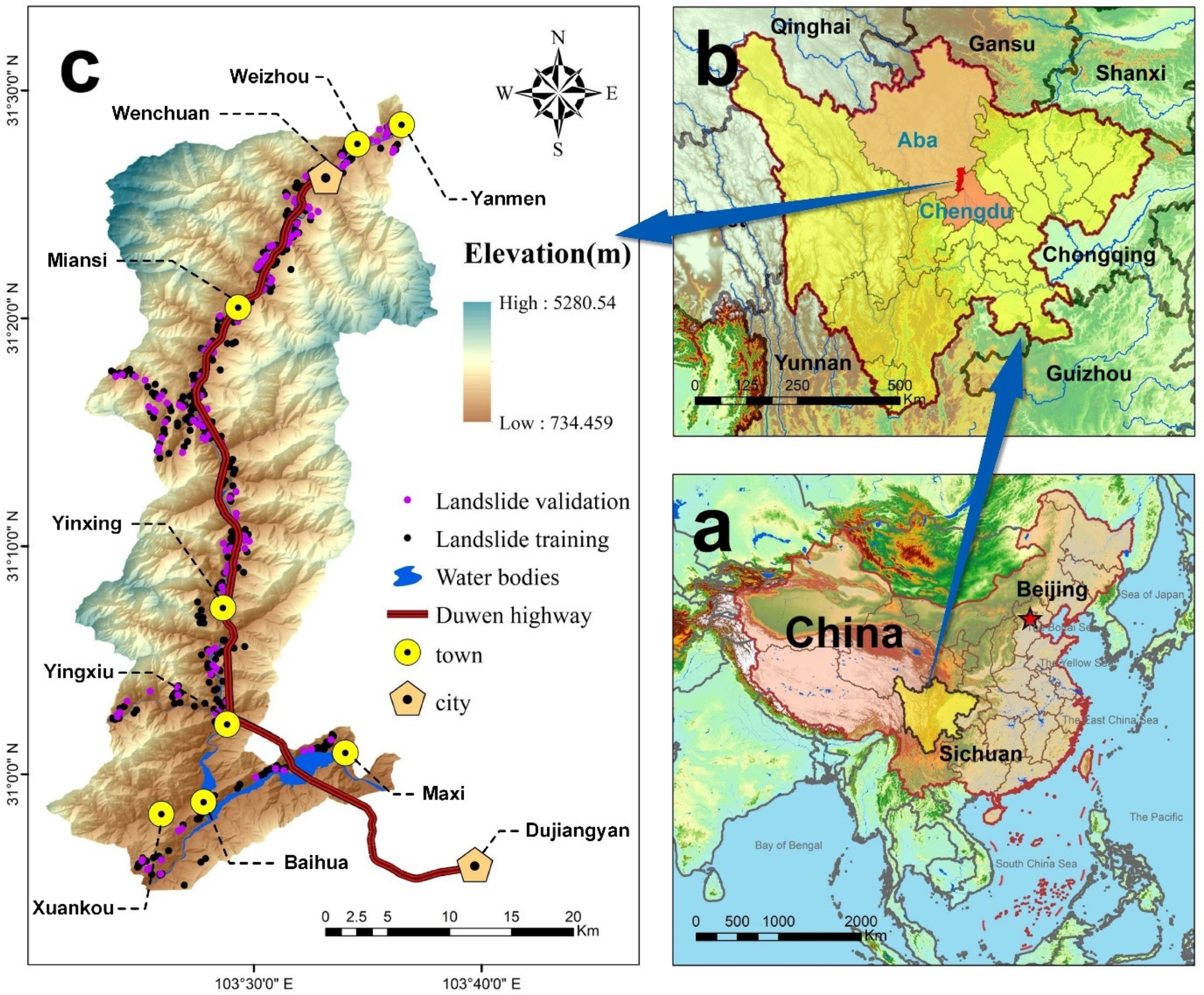
2.1. Study Area
2.2. Landslide Inventory
2.3. Landslide Influencing Factors
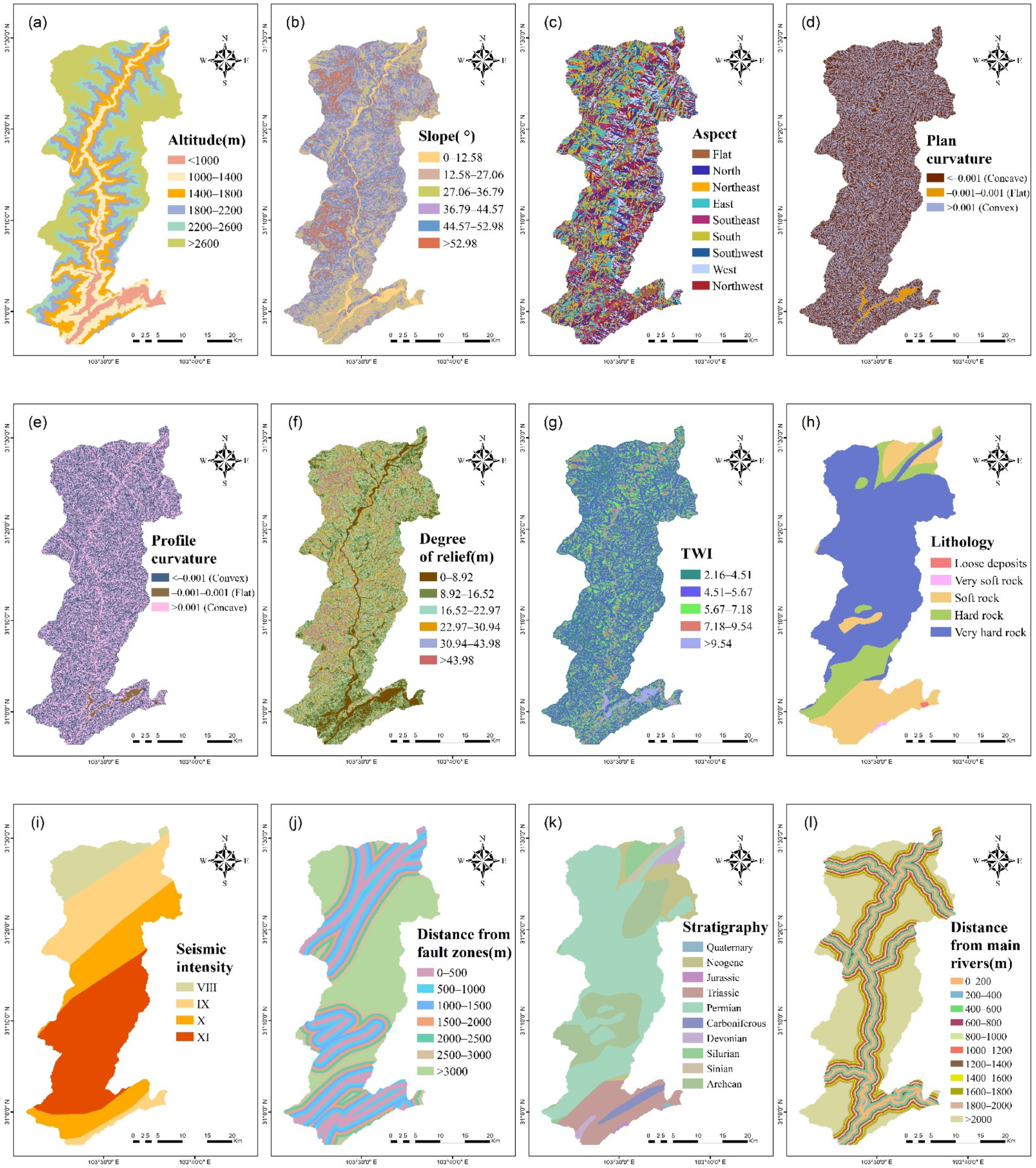
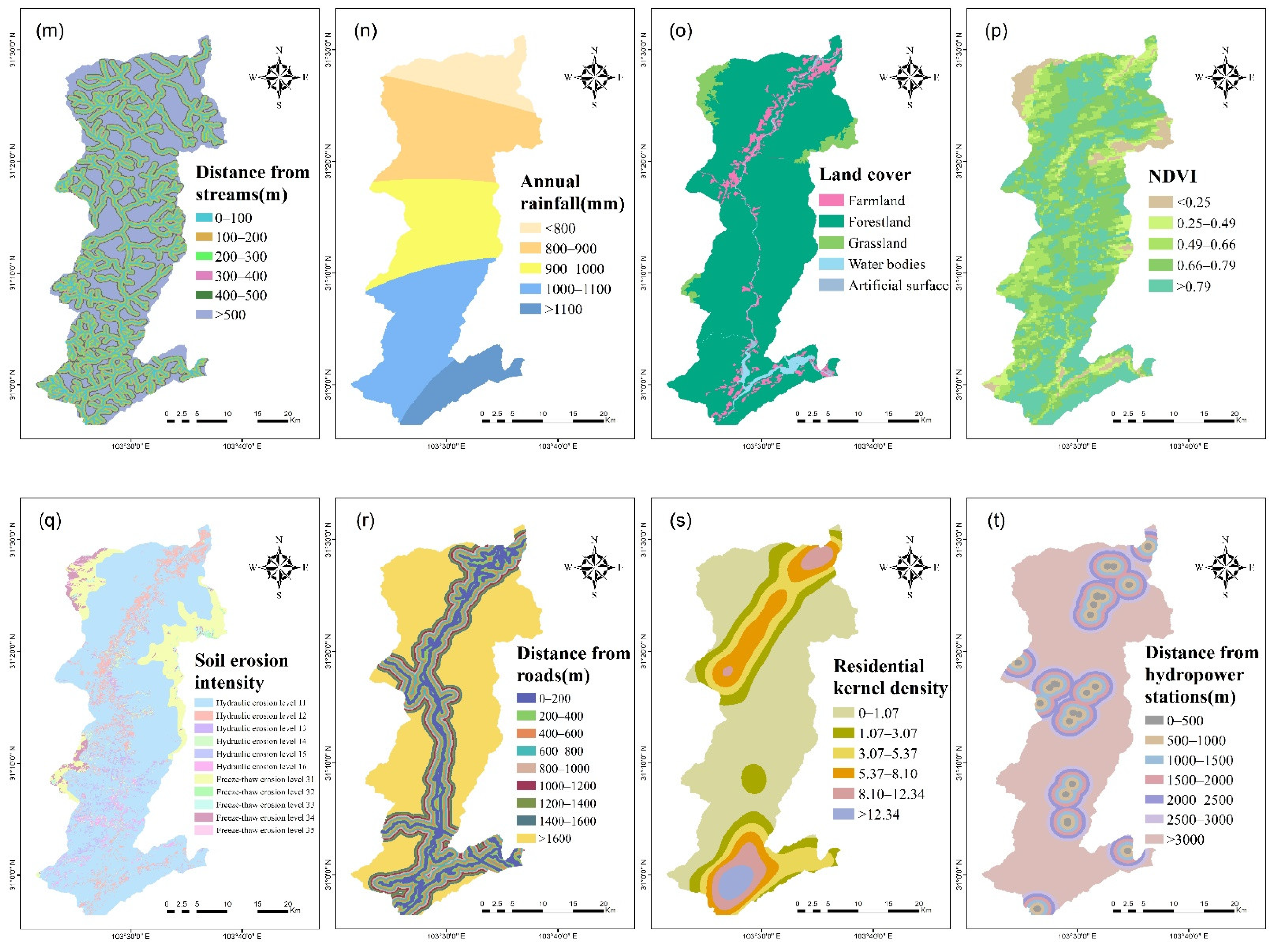
2.3.1. Topographic Factors
2.3.2. Geological Factors
2.3.3. Ecological Factors
2.3.4. Human Engineering Activity Factors
3. Methods
3.1. Statistical Index
3.2. GeoDetector
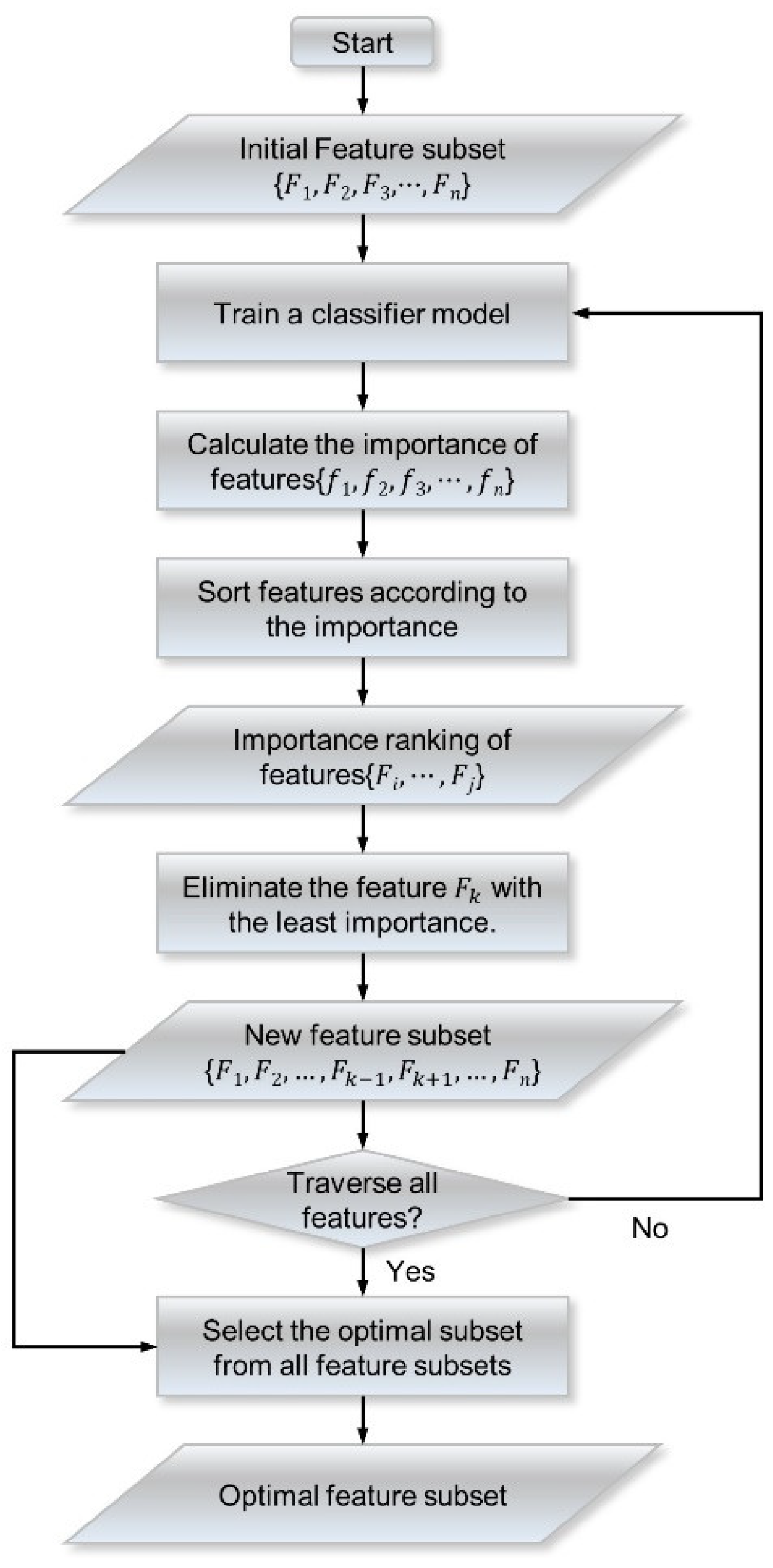
3.3. Recursive Feature Elimination
3.4. Gaussian Process Regression
3.5. Model Validation Method
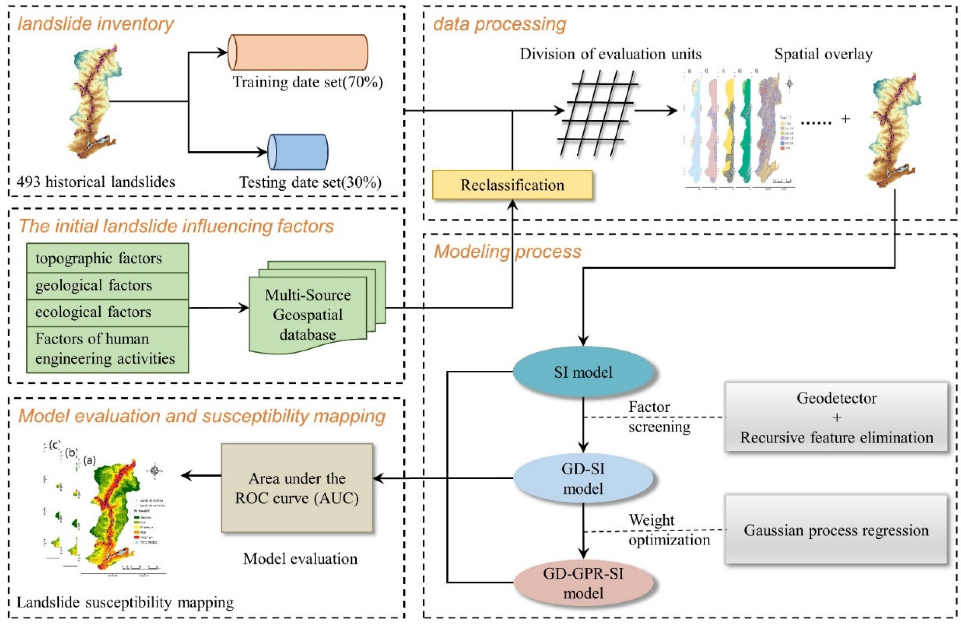
4. Modeling Process and Results
4.1. Implementation of SI
4.2. Construction of the GD-SI Model
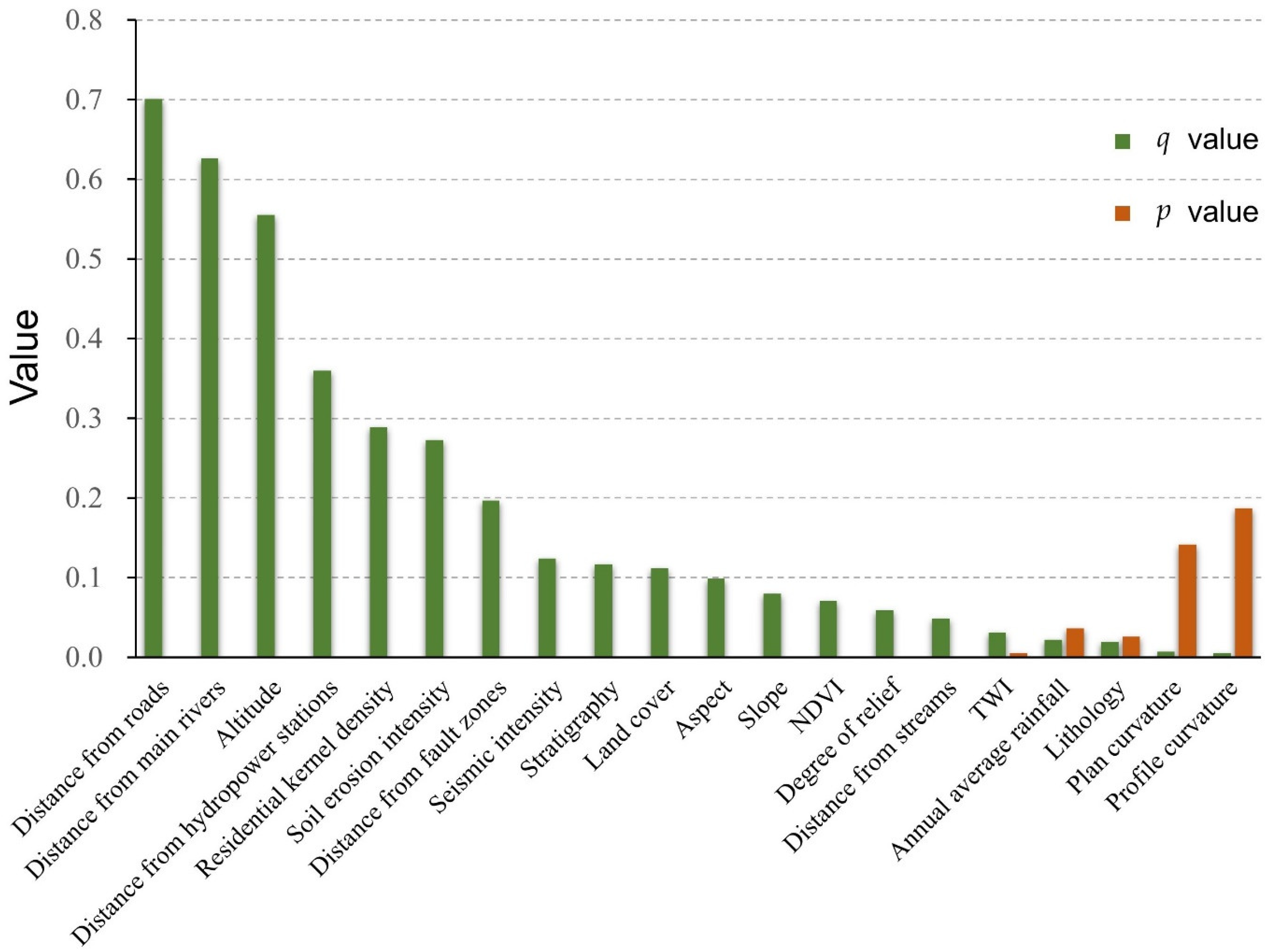
4.2.1. GeoDetector Result
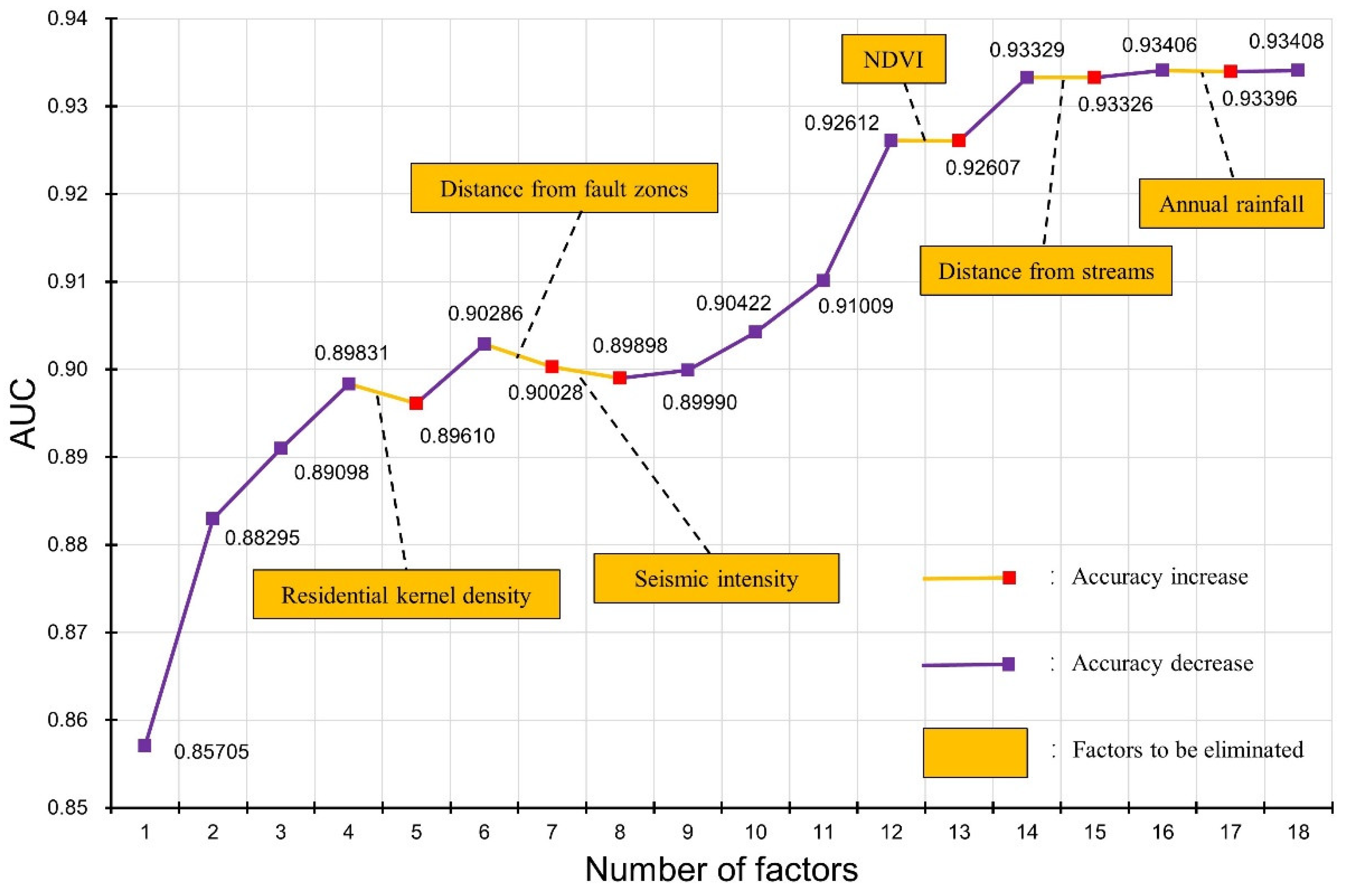
4.2.2. Factor Screening Based on GD and RFE
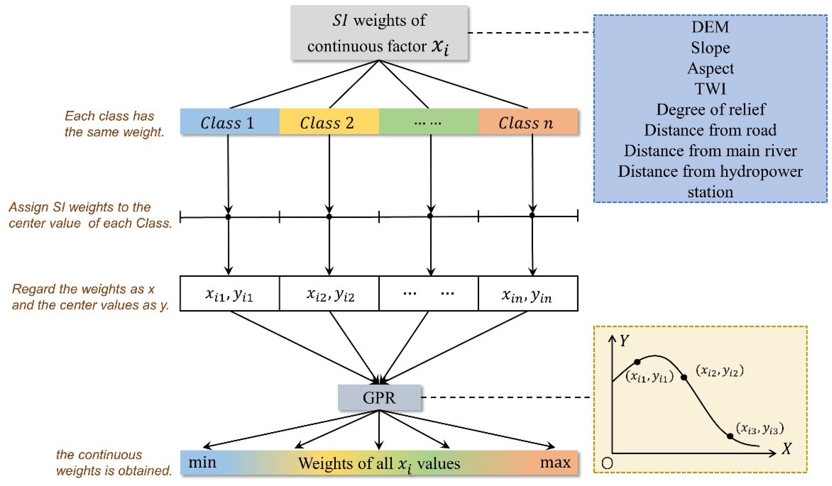
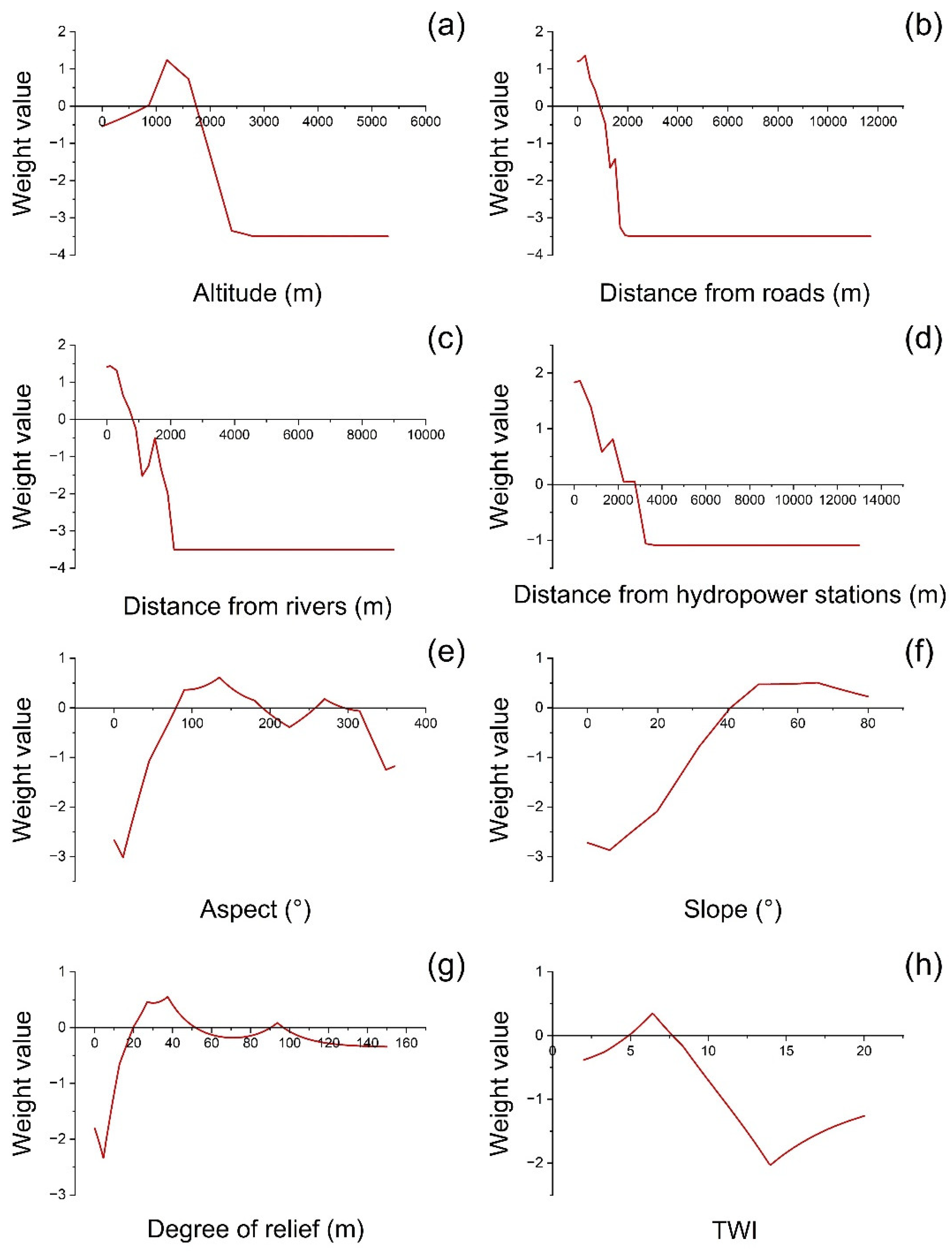
4.3. Construction of the GD-GPR-SI Model
4.4. Correlation between Selected Factors and Landslide
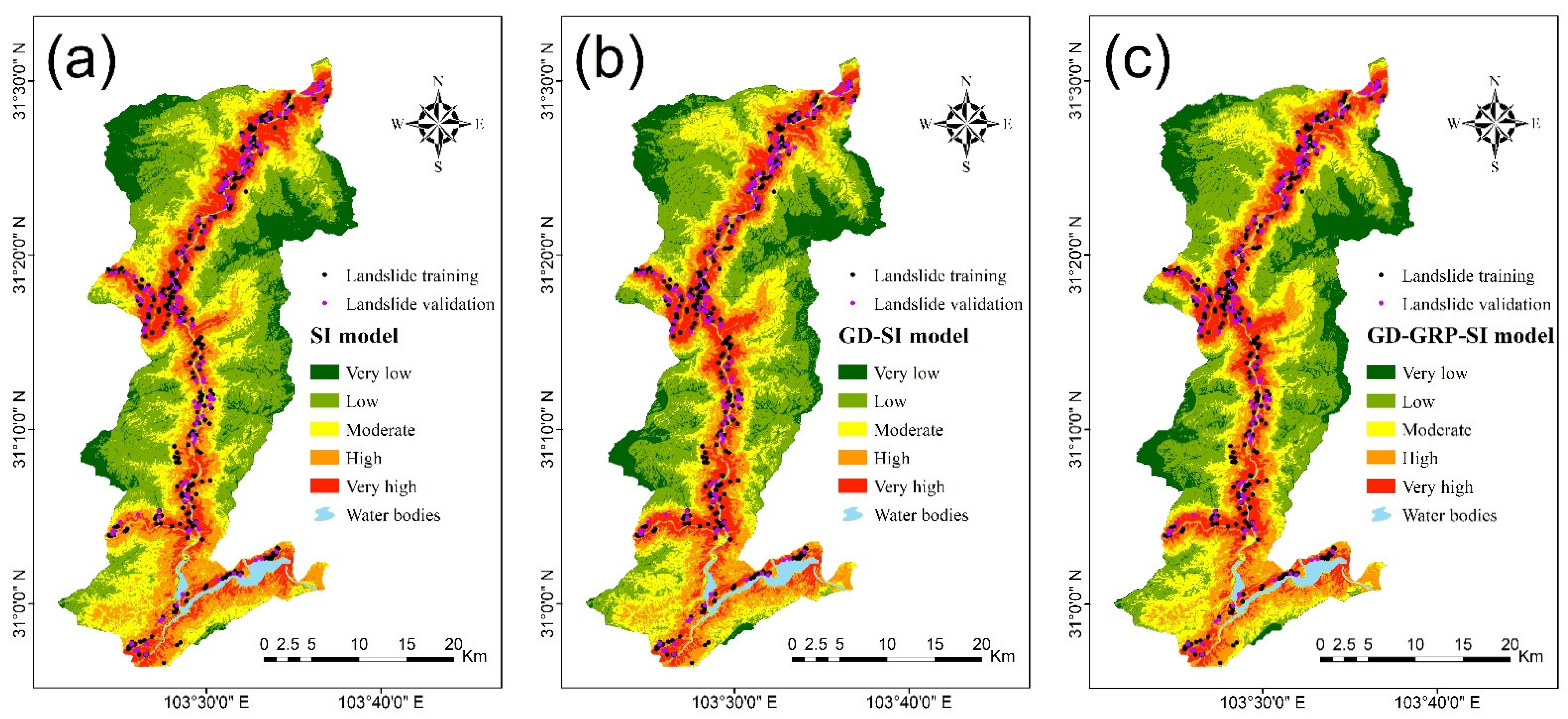
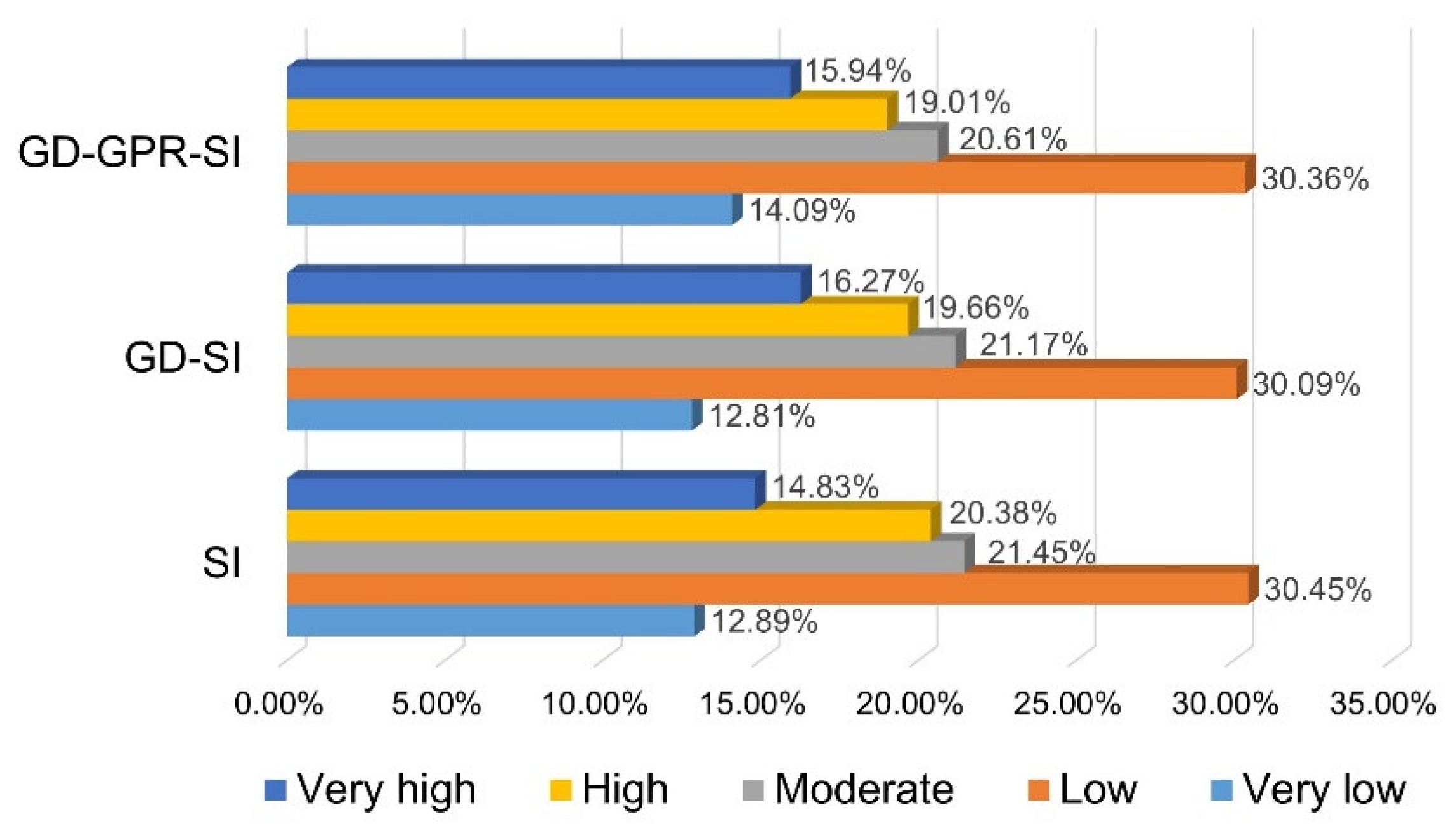
4.5. Landslide Susceptibility Mapping
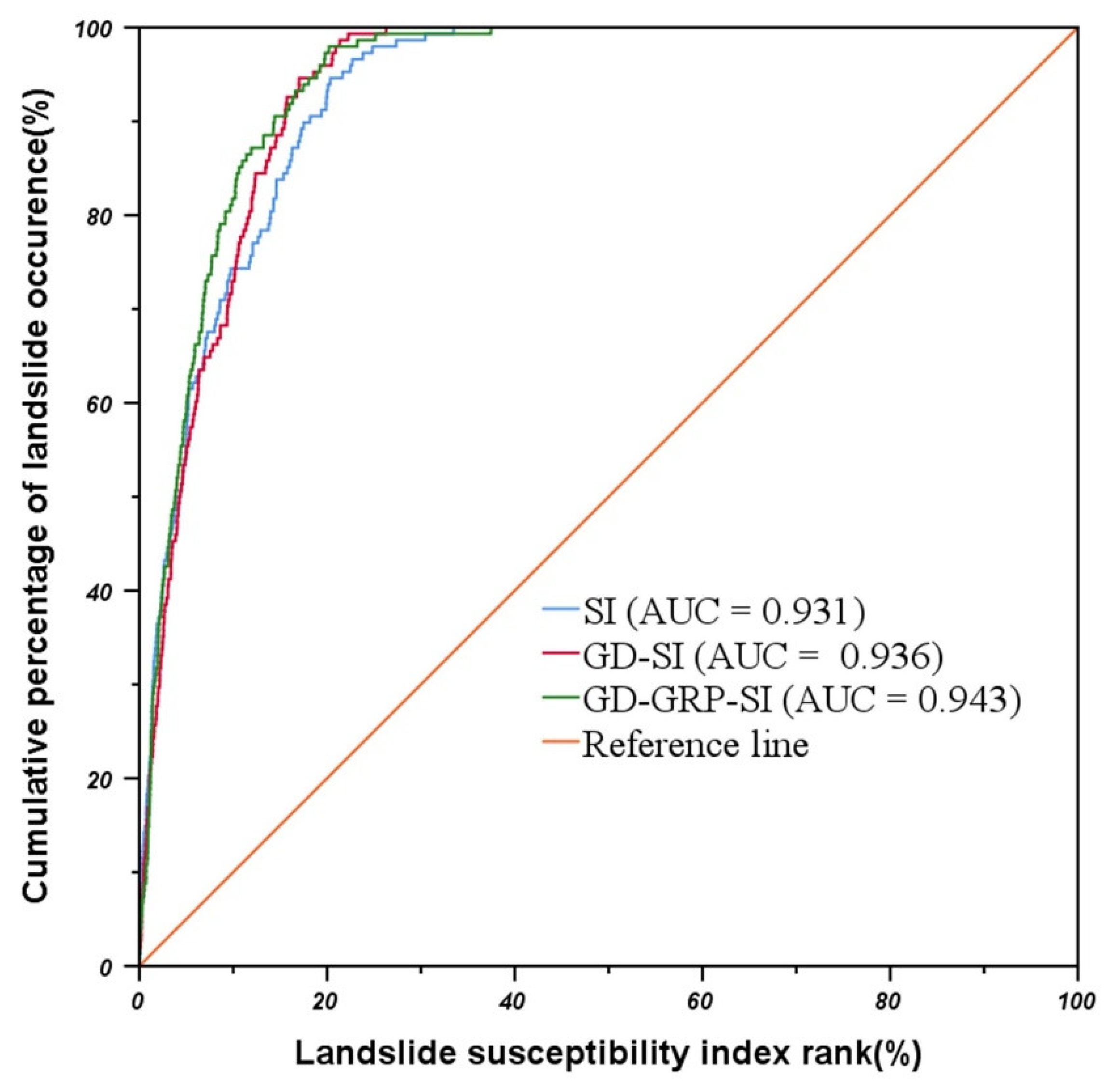
4.6. Validation of Models
5. Discussion
5.1. The Dominant Factors of Landslides in the Study Area
5.2. Advantages of the Hybrid Model
5.3. Limitations of This Study and Prospects of Future Research
6. Conclusions
Author Contributions
Funding
Institutional Review Board Statement
Informed Consent Statement
Data Availability Statement
Acknowledgments
Conflicts of Interest
References
- Cruden, D.M. A simple definition of a landslide. Bull. Int. Assoc. Eng. Geol. 1991, 43, 27–29. [Google Scholar] [CrossRef]
- Petley, D. Global patterns of loss of life from landslides. Geology 2012, 40, 927–930. [Google Scholar] [CrossRef]
- Froude, M.J.; Petley, D.N. Global fatal landslide occurrence from 2004 to 2016. Nat. Hazard Earth Syst. 2018, 18, 2161–2181. [Google Scholar] [CrossRef]
- Reichenbach, P.; Rossi, M.; Malamud, B.D.; Mihir, M.; Guzzetti, F. A review of statistically-based landslide susceptibility models. Earth-Sci. Rev. 2018, 180, 60–91. [Google Scholar] [CrossRef]
- Merghadi, A.; Yunus, A.P.; Dou, J.; Whiteley, J.; ThaiPham, B.; Bui, D.T.; Avtar, R.; Abderrahmane, B. Machine learning methods for landslide susceptibility studies: A comparative overview of algorithm performance. Earth-Sci. Rev. 2020, 207, 103225. [Google Scholar] [CrossRef]
- Piciullo, L.; Calvello, M.; Cepeda, J.M. Territorial early warning systems for rainfall-induced landslides. Earth-Sci. Rev. 2018, 179, 228–247. [Google Scholar] [CrossRef]
- Shinoda, M.; Miyata, Y.; Kurokawa, U.; Kondo, K. Regional landslide susceptibility following the 2016 Kumamoto earthquake using back-calculated geomaterial strength parameters. Landslides 2019, 16, 1497–1516. [Google Scholar] [CrossRef]
- Panchal, S.; Shrivastava, A.K. A Comparative Study of Frequency Ratio, Shannon’s Entropy and Analytic Hierarchy Process (AHP) Models for Landslide Susceptibility Assessment. ISPRS Int. J. Geo-Inf. 2021, 10, 603. [Google Scholar] [CrossRef]
- Dehnavi, A.; Aghdam, I.N.; Pradhan, B.; Varzandeh, M.H.M. A new hybrid model using step-wise weight assessment ratio analysis (SWAM) technique and adaptive neuro-fuzzy inference system (ANFIS) for regional landslide hazard assessment in Iran. Catena 2015, 135, 122–148. [Google Scholar] [CrossRef]
- Gheshlaghi, H.A.; Feizizadeh, B. An integrated approach of analytical network process and fuzzy based spatial decision making systems applied to landslide risk mapping. J. Afr. Earth Sci. 2017, 133, 15–24. [Google Scholar] [CrossRef]
- Zare, N.; Hosseini, S.A.O.; Hafizi, M.K.; Najafi, A.; Majnounian, B.; Geertsema, M. A Comparison of an Adaptive Neuro-Fuzzy and Frequency Ratio Model to Landslide-Susceptibility Mapping along Forest Road Networks. Forests 2021, 12, 1087. [Google Scholar] [CrossRef]
- Luo, W.; Liu, C.C. Innovative landslide susceptibility mapping supported by geomorphon and geographical detector methods. Landslides 2018, 15, 465–474. [Google Scholar] [CrossRef]
- Wang, Q.; Li, W.; Wu, Y.; Pei, Y.; Xie, P. Application of statistical index and index of entropy methods to landslide susceptibility assessment in Gongliu (Xinjiang, China). Environ. Earth Sci. 2016, 75, 599. [Google Scholar] [CrossRef]
- Zhao, X.; Chen, W. GIS-Based Evaluation of Landslide Susceptibility Models Using Certainty Factors and Functional Trees-Based Ensemble Techniques. Appl. Sci. 2020, 10, 16. [Google Scholar] [CrossRef]
- Batar, A.K.; Watanabe, T. Landslide Susceptibility Mapping and Assessment Using Geospatial Platforms and Weights of Evidence (WoE) Method in the Indian Himalayan Region: Recent Developments, Gaps, and Future Directions. ISPRS Int. J. Geo-Inf. 2021, 10, 114. [Google Scholar] [CrossRef]
- Viet-Ha, N.; Mohammadi, A.; Shahabi, H.; Bin Ahmad, B.; Al-Ansari, N.; Shirzadi, A.; Geertsema, M.; Kress, V.R.; Karimzadeh, S.; Kamran, K.V.; et al. Landslide Detection and Susceptibility Modeling on Cameron Highlands (Malaysia): A Comparison between Random Forest, Logistic Regression and Logistic Model Tree Algorithms. Forests 2020, 11, 830. [Google Scholar] [CrossRef]
- Kalantar, B.; Pradhan, B.; Naghibi, S.A.; Motevalli, A.; Mansor, S. Assessment of the effects of training data selection on the landslide susceptibility mapping: A comparison between support vector machine (SVM), logistic regression (LR) and artificial neural networks (ANN). Geomat. Nat. Hazards Risk 2018, 9, 49–69. [Google Scholar] [CrossRef]
- Viet-Ha, N.; Shirzadi, A.; Shahabi, H.; Chen, W.; Clague, J.J.; Geertsema, M.; Jaafari, A.; Avand, M.; Miraki, S.; Asl, D.T.; et al. Shallow Landslide Susceptibility Mapping by Random Forest Base Classifier and Its Ensembles in a Semi-Arid Region of Iran. Forests 2020, 11, 421. [Google Scholar] [CrossRef]
- Viet-Hung, D.; Nhat-Duc, H.; Le-Mai-Duyen, N.; Dieu Tien, B.; Samui, P. A Novel GIS-Based Random Forest Machine Algorithm for the Spatial Prediction of Shallow Landslide Susceptibility. Forests 2020, 11, 118. [Google Scholar] [CrossRef]
- Zhang, W.; Liu, S.; Wang, L.; Samui, P.; Chwala, M.; He, Y. Landslide Susceptibility Research Combining Qualitative Analysis and Quantitative Evaluation: A Case Study of Yunyang County in Chongqing, China. Forests 2022, 13, 1055. [Google Scholar] [CrossRef]
- Dieu Tien, B.; Shirzadi, A.; Shahabi, H.; Geertsema, M.; Omidvar, E.; Clague, J.J.; Binh Thai, P.; Dou, J.; Asl, D.T.; Bin Ahmad, B.; et al. New Ensemble Models for Shallow Landslide Susceptibility Modeling in a Semi-Arid Watershed. Forests 2019, 10, 743. [Google Scholar] [CrossRef]
- Xie, W.; Nie, W.; Saffari, P.; Robledo, L.F.; Descote, P.-Y.; Jian, W. Landslide hazard assessment based on Bayesian optimization-support vector machine in Nanping City, China. Nat. Hazards 2021, 109, 931–948. [Google Scholar] [CrossRef]
- Vu Viet, N.; Binh Thai, P.; Ba Thao, V.; Prakash, I.; Jha, S.; Shahabi, H.; Shirzadi, A.; Dong Nguyen, B.; Kumar, R.; Chatterjee, J.M.; et al. Hybrid Machine Learning Approaches for Landslide Susceptibility Modeling. Forests 2019, 10, 157. [Google Scholar] [CrossRef]
- Kawabata, D.; Bandibas, J. Landslide susceptibility mapping using geological data, a DEM from ASTER images and an Artificial Neural Network (ANN). Geomorphology 2009, 113, 97–109. [Google Scholar] [CrossRef]
- Chen, W.; Xie, X.S.; Peng, J.B.; Shahabi, H.; Hong, H.Y.; Bui, D.T.; Duan, Z.; Li, S.J.; Zhu, A.X. GIS-based landslide susceptibility evaluation using a novel hybrid integration approach of bivariate statistical based random forest method. Catena 2018, 164, 135–149. [Google Scholar] [CrossRef]
- Chen, W.; Sun, Z.H.; Han, J.C. Landslide Susceptibility Modeling Using Integrated Ensemble Weights of Evidence with Logistic Regression and Random Forest Models. Appl. Sci. 2019, 9, 171. [Google Scholar] [CrossRef]
- Chen, L.; Guo, H.; Gong, P.; Yang, Y.; Zuo, Z.; Gu, M. Landslide susceptibility assessment using weights-of-evidence model and cluster analysis along the highways in the Hubei section of the Three Gorges Reservoir Area. Comput. Geosci. 2021, 156, 104899. [Google Scholar] [CrossRef]
- Jaafari, A.; Najafi, A.; Pourghasemi, H.R.; Rezaeian, J.; Sattarian, A. GIS-based frequency ratio and index of entropy models for landslide susceptibility assessment in the Caspian forest, northern Iran. Int. J. Environ. Sci. 2014, 11, 909–926. [Google Scholar] [CrossRef]
- Yong, C.; Dong, J.; Fei, G.; Bin, T.; Tao, Z.; Hao, F.; Li, W.; Qinghua, Z. Review of landslide susceptibility assessment based on knowledge mapping. Stoch. Environ. Res. Risk Assess. 2022, 36, 2399–2417. [Google Scholar] [CrossRef]
- Chen, W.; Chen, X.; Peng, J.B.; Panahi, M.; Lee, S. Landslide susceptibility modeling based on ANFIS with teaching-learning-based optimization and Satin bowerbird optimizer. Geosci. Front. 2021, 12, 93–107. [Google Scholar] [CrossRef]
- Tobler, W.R. A Computer Movie Simulating Urban Growth in the Detroit Region. Econ. Geogr. 1970, 46, 234–240. [Google Scholar] [CrossRef]
- Aghdam, I.N.; Pradhan, B.; Panahi, M. Landslide susceptibility assessment using a novel hybrid model of statistical bivariate methods (FR and WOE) and adaptive neuro-fuzzy inference system (ANFIS) at southern Zagros Mountains in Iran. Environ. Earth Sci. 2017, 76, 237. [Google Scholar] [CrossRef]
- Aghdam, I.N.; Varzandeh, M.H.M.; Pradhan, B. Landslide susceptibility mapping using an ensemble statistical index (Wi) and adaptive neuro-fuzzy inference system (ANFIS) model at Alborz Mountains (Iran). Environ. Earth Sci. 2016, 75, 553. [Google Scholar] [CrossRef]
- Jebur, M.N.; Pradhan, B.; Tehrany, M.S. Optimization of landslide conditioning factors using very high-resolution airborne laser scanning (LiDAR) data at catchment scale. Remote Sens. Environ. 2014, 152, 150–165. [Google Scholar] [CrossRef]
- Zhou, C.; Yin, K.L.; Cao, Y.; Ahmed, B.; Li, Y.Y.; Catani, F.; Pourghasemi, H.R. Landslide susceptibility modeling applying machine learning methods: A case study from Longju in the Three Gorges Reservoir area, China. Comput. Geosci. 2018, 112, 23–37. [Google Scholar] [CrossRef]
- Chen, X.; Chen, W. GIS-based landslide susceptibility assessment using optimized hybrid machine learning methods. Catena 2021, 196, 104833. [Google Scholar] [CrossRef]
- Sun, D.L.; Wen, H.J.; Wang, D.Z.; Xu, J.H. A random forest model of landslide susceptibility mapping based on hyperparameter optimization using Bayes algorithm. Geomorphology 2020, 362, 107201. [Google Scholar] [CrossRef]
- Liu, J.P.; Zeng, Z.P.; Liu, H.Q.; Wang, H.B. A rough set approach to analyze factors affecting landslide incidence. Comput. Geosci. 2011, 37, 1311–1317. [Google Scholar] [CrossRef]
- Li, L.M.; Cheng, S.K.; Wen, Z.Z. Landslide prediction based on improved principal component analysis and mixed kernel function least squares support vector regression model. J. Mt. Sci. 2021, 18, 2130–2142. [Google Scholar] [CrossRef]
- Zhang, T.Y.; Han, L.; Chen, W.; Shahabi, H. Hybrid Integration Approach of Entropy with Logistic Regression and Support Vector Machine for Landslide Susceptibility Modeling. Entropy 2018, 20, 884. [Google Scholar] [CrossRef]
- Wu, Y.L.; Ke, Y.T.; Chen, Z.; Liang, S.Y.; Zhao, H.L.; Hong, H.Y. Application of alternating decision tree with AdaBoost and bagging ensembles for landslide susceptibility mapping. Catena 2020, 187, 104396. [Google Scholar] [CrossRef]
- Wang, J.F.; Li, X.H.; Christakos, G.; Liao, Y.L.; Zhang, T.; Gu, X.; Zheng, X.Y. Geographical Detectors-Based Health Risk Assessment and its Application in the Neural Tube Defects Study of the Heshun Region, China. Int. J. Geogr. Inf. Sci. 2010, 24, 107–127. [Google Scholar] [CrossRef]
- Wang, J.F.; Zhang, T.L.; Fu, B.J. A measure of spatial stratified heterogeneity. Ecol. Indic. 2016, 67, 250–256. [Google Scholar] [CrossRef]
- Xie, W.; Li, X.S.; Jian, W.B.; Yang, Y.; Liu, H.W.; Robledo, L.F.; Nie, W. A Novel Hybrid Method for Landslide Susceptibility Mapping-Based GeoDetector and Machine Learning Cluster: A Case of Xiaojin County, China. ISPRS Int. J. Geo-Inf. 2021, 10, 93. [Google Scholar] [CrossRef]
- Yang, J.T.; Song, C.; Yang, Y.; Xu, C.D.; Guo, F.; Xie, L. New method for landslide susceptibility mapping supported by spatial logistic regression and GeoDetector: A case study of Duwen Highway Basin, Sichuan Province, China. Geomorphology 2019, 324, 62–71. [Google Scholar] [CrossRef]
- Yin, Y.P.; Wang, F.W.; Sun, P. Landslide hazards triggered by the 2008 Wenchuan earthquake, Sichuan, China. Landslides 2009, 6, 139–152. [Google Scholar] [CrossRef]
- Yang, Y.; Yang, J.T.; Xu, C.D.; Xu, C.; Song, C. Local-scale landslide susceptibility mapping using the B-GeoSVC model. Landslides 2019, 16, 1301–1312. [Google Scholar] [CrossRef]
- Zhang, H.Z.; Chi, T.H.; Fan, J.R.; Hu, K.H.; Peng, L. Spatial Analysis of Wenchuan Earthquake-Damaged Vegetation in the Mountainous Basins and Its Applications. Remote Sens. 2015, 7, 5785–5804. [Google Scholar] [CrossRef]
- Hungr, O.; Leroueil, S.; Picarelli, L. The Varnes classification of landslide types, an update. Landslides 2014, 11, 167–194. [Google Scholar] [CrossRef]
- Hong, H.Y.; Pourghasemi, H.R.; Pourtaghi, Z.S. Landslide susceptibility assessment in Lianhua County (China): A comparison between a random forest data mining technique and bivariate and multivariate statistical models. Geomorphology 2016, 259, 105–118. [Google Scholar] [CrossRef]
- Wang, Y.; Sun, D.L.; Wen, H.J.; Zhang, H.; Zhang, F.T. Comparison of Random Forest Model and Frequency Ratio Model for Landslide Susceptibility Mapping (LSM) in Yunyang County (Chongqing, China). Int. J. Environ. Res. Public Health 2020, 17, 4206. [Google Scholar] [CrossRef] [PubMed]
- Zhou, X.Z.; Wen, H.J.; Zhang, Y.L.; Xu, J.H.; Zhang, W.G. Landslide susceptibility mapping using hybrid random forest with GeoDetector and RFE for factor optimization. Geosci. Front. 2021, 12, 101211. [Google Scholar] [CrossRef]
- Chen, W.; Pourghasemi, H.R.; Panahi, M.; Kornejady, A.; Wang, J.L.; Xie, X.S.; Cao, S.B. Spatial prediction of landslide susceptibility using an adaptive neuro-fuzzy inference system combined with frequency ratio, generalized additive model, and support vector machine techniques. Geomorphology 2017, 297, 69–85. [Google Scholar] [CrossRef]
- Sun, D.L.; Shi, S.X.; Wen, H.J.; Xu, J.H.; Zhou, X.Z.; Wu, J.P. A hybrid optimization method of factor screening predicated on GeoDetector and Random Forest for Landslide Susceptibility Mapping. Geomorphology 2021, 379, 107623. [Google Scholar] [CrossRef]
- Bui, D.T.; Lofman, O.; Revhaug, I.; Dick, O. Landslide susceptibility analysis in the Hoa Binh province of Vietnam using statistical index and logistic regression. Nat Hazards 2011, 59, 1413–1444. [Google Scholar] [CrossRef]
- Zhao, Y.; Wang, R.; Jiang, Y.J.; Liu, H.J.; Wei, Z.L. GIS-based logistic regression for rainfall-induced landslide susceptibility mapping under different grid sizes in Yueqing, Southeastern China. Eng. Geol. 2019, 259, 105147. [Google Scholar] [CrossRef]
- Xu, C.; Xu, X.W.; Yao, X.; Dai, F.C. Three (nearly) complete inventories of landslides triggered by the May 12, 2008 Wenchuan Mw 7.9 earthquake of China and their spatial distribution statistical analysis. Landslides 2014, 11, 441–461. [Google Scholar] [CrossRef]
- Balogun, A.L.; Rezaie, F.; Pham, Q.B.; Gigovic, L.; Drobnjak, S.; Aina, Y.A.; Panahi, M.; Yekeen, S.T.; Lee, S. Spatial prediction of landslide susceptibility in western Serbia using hybrid support vector regression (SVR) with GWO, BAT and COA algorithms. Geosci. Front. 2021, 12, 101104. [Google Scholar] [CrossRef]
- Dou, J.; Yunus, A.P.; Dieu Tien, B.; Sahana, M.; Chen, C.-W.; Zhu, Z.; Wang, W.; Binh Thai, P. Evaluating GIS-Based Multiple Statistical Models and Data Mining for Earthquake and Rainfall-Induced Landslide Susceptibility Using the LiDAR DEM. Remote Sens. 2019, 11, 638. [Google Scholar] [CrossRef]
- Liu, L.; Xu, C.; Xu, X.; Tian, Y.; Ran, Y.; Chen, J. Interactive statistical analysis of predisposing factors for earthquake-triggered landslides: A case study of the 2013 Lushan, China Ms7.0 earthquake. Environ. Earth Sci. 2015, 73, 4729–4738. [Google Scholar] [CrossRef]
- Merghadi, A.; Abderrahmane, B.; Dieu Tien, B. Landslide Susceptibility Assessment at Mila Basin (Algeria): A Comparative Assessment of Prediction Capability of Advanced Machine Learning Methods. ISPRS Int. J. Geo-Inf. 2018, 7, 268. [Google Scholar] [CrossRef]
- Deng, H.; Wu, L.Z.; Huang, R.Q.; Guo, X.G.; He, Q. Formation of the Siwanli ancient landslide in the Dadu River, China. Landslides 2017, 14, 385–394. [Google Scholar] [CrossRef]
- Juliev, M.; Mergili, M.; Mondal, I.; Nurtaev, B.; Pulatov, A.; Hubl, J. Comparative analysis of statistical methods for landslide susceptibility mapping in the Bostanlik District, Uzbekistan. Sci. Total Environ. 2019, 653, 801–814. [Google Scholar] [CrossRef]
- Wang, X.; Huang, Z.; Hong, M.M.M.; Zhao, Y.F.; Ou, Y.S.; Zhang, J. A comparison of the effects of natural vegetation regrowth with a plantation scheme on soil structure in a geological hazard-prone region. Eur. J. Soil Sci. 2019, 70, 674–685. [Google Scholar] [CrossRef]
- Huang, F.M.; Chen, J.W.; Du, Z.; Yao, C.; Huang, J.S.; Jiang, Q.H.; Chang, Z.L.; Li, S. Landslide Susceptibility Prediction Considering Regional Soil Erosion Based on Machine-Learning Models. ISPRS Int. J. Geo-Inf. 2020, 9, 377. [Google Scholar] [CrossRef]
- Pradhan, B.; Chaudhari, A.; Adinarayana, J.; Buchroithner, M.F. Soil erosion assessment and its correlation with landslide events using remote sensing data and GIS: A case study at Penang Island, Malaysia. Environ. Monit. Assess. 2012, 184, 715–727. [Google Scholar] [CrossRef] [PubMed]
- Duan, X.W.; Liu, B.; Gu, Z.J.; Rong, L.; Feng, D.T. Quantifying soil erosion effects on soil productivity in the dry-hot valley, southwestern China. Environ. Earth Sci. 2016, 75, 1164. [Google Scholar] [CrossRef]
- Zhang, G.F.; Cai, Y.X.; Zheng, Z.; Zhen, J.W.; Liu, Y.L.; Huang, K.Y. Integration of the Statistical Index Method and the Analytic Hierarchy Process technique for the assessment of landslide susceptibility in Huizhou, China. Catena 2016, 142, 233–244. [Google Scholar] [CrossRef]
- Yalcin, A.; Reis, S.; Aydinoglu, A.C.; Yomralioglu, T. A GIS-based comparative study of frequency ratio, analytical hierarchy process, bivariate statistics and logistics regression methods for landslide susceptibility mapping in Trabzon, NE Turkey. Catena 2011, 85, 274–287. [Google Scholar] [CrossRef]
- Arabameri, A.; Pradhan, B.; Rezaei, K.; Lee, C.W. Assessment of Landslide Susceptibility Using Statistical- and Artificial Intelligence-Based FR-RF Integrated Model and Multiresolution DEMs. Remote Sens. 2019, 11, 999. [Google Scholar] [CrossRef]
- Zhou, J.W.; Lu, P.Y.; Yang, Y.C. Reservoir Landslides and Its Hazard Effects for the Hydropower Station: A Case Study. In Advancing Culture of Living with Landslides, Vol 2: Advances in Landslide Science; Springer: Cham, Switzerland, 2017; pp. 699–706. [Google Scholar] [CrossRef]
- Xia, M.; Ren, G.M.; Zhu, S.S.; Ma, X.L. Relationship between landslide stability and reservoir water level variation. Bull. Eng. Geol. Environ. 2015, 74, 909–917. [Google Scholar] [CrossRef]
- Regmi, A.D.; Devkota, K.C.; Yoshida, K.; Pradhan, B.; Pourghasemi, H.R.; Kumamoto, T.; Akgun, A. Application of frequency ratio, statistical index, and weights-of-evidence models and their comparison in landslide susceptibility mapping in Central Nepal Himalaya. Arab. J. Geosci. 2014, 7, 725–742. [Google Scholar] [CrossRef]
- Chen, W.; Shahabi, H.; Shirzadi, A.; Hong, H.Y.; Akgun, A.; Tian, Y.Y.; Liu, J.Z.; Zhu, A.X.; Li, S.J. Novel hybrid artificial intelligence approach of bivariate statistical-methods-based kernel logistic regression classifier for landslide susceptibility modeling. Bull. Eng. Geol. Environ. 2019, 78, 4397–4419. [Google Scholar] [CrossRef]
- Guyon, I.; Weston, J.; Barnhill, S.; Vapnik, V. Gene Selection for Cancer Classification using Support Vector Machines. Mach. Learn. 2002, 46, 389–422. [Google Scholar] [CrossRef]
- Sheng, H.M.; Xiao, J.; Cheng, Y.H.; Ni, Q.; Wang, S. Short-Term Solar Power Forecasting Based on Weighted Gaussian Process Regression. IEEE Trans. Ind. Electron. 2018, 65, 300–308. [Google Scholar] [CrossRef]
- Liu, K.L.; Hu, X.S.; Wei, Z.B.; Li, Y.; Jiang, Y. Modified Gaussian Process Regression Models for Cyclic Capacity Prediction of Lithium-Ion Batteries. IEEE Trans. Transp. Electr. 2019, 5, 1225–1236. [Google Scholar] [CrossRef]
- Zhou, Y.; Liu, Y.F.; Wang, D.J.; De, G.; Li, Y.; Liu, X.J.; Wang, Y.Y. A novel combined multi-task learning and Gaussian process regression model for the prediction of multi-timescale and multi-component of solar radiation. J. Clean. Prod. 2021, 284, 124710. [Google Scholar] [CrossRef]
- Li, X.Y.; Yuan, C.G.; Li, X.H.; Wang, Z.P. State of health estimation for Li-Ion battery using incremental capacity analysis and Gaussian process regression. Energy 2020, 190, 116467. [Google Scholar] [CrossRef]
- Bui, D.T.; Pradhan, B.; Lofman, O.; Revhaug, I.; Dick, O.B. Landslide susceptibility mapping at Hoa Binh province (Vietnam) using an adaptive neuro-fuzzy inference system and GIS. Comput. Geosci. 2012, 45, 199–211. [Google Scholar] [CrossRef]
- Pourghasemi, H.R.; Moradi, H.R.; Aghda, S.M.F. Landslide susceptibility mapping by binary logistic regression, analytical hierarchy process, and statistical index models and assessment of their performances. Nat. Hazards 2013, 69, 749–779. [Google Scholar] [CrossRef]
- Wu, R.; Zhang, Y.; Guo, C.; Yang, Z.; Tang, J.; Su, F. Landslide susceptibility assessment in mountainous area: A case study of Sichuan-Tibet railway, China. Environ. Earth Sci. 2020, 79, 157. [Google Scholar] [CrossRef]
- Lee, S.; Talib, J.A. Probabilistic landslide susceptibility and factor effect analysis. Environ. Geol. 2005, 47, 982–990. [Google Scholar] [CrossRef]
- Devkota, K.C.; Regmi, A.D.; Pourghasemi, H.R.; Yoshida, K.; Pradhan, B.; Ryu, I.C.; Dhital, M.R.; Althuwaynee, O.F. Landslide susceptibility mapping using certainty factor, index of entropy and logistic regression models in GIS and their comparison at Mugling-Narayanghat road section in Nepal Himalaya. Nat. Hazards 2013, 65, 135–165. [Google Scholar] [CrossRef]
- Achour, Y.; Pourghasemi, H.R. How do machine learning techniques help in increasing accuracy of landslide susceptibility maps? Geosci. Front. 2020, 11, 871–883. [Google Scholar] [CrossRef]
- Zhao, B.; Ge, Y.; Chen, H. Landslide susceptibility assessment for a transmission line in Gansu Province, China by using a hybrid approach of fractal theory, information value, and random forest models. Environ. Earth Sci. 2021, 80, 441. [Google Scholar] [CrossRef]
- Chiessi, V.; Toti, S.; Vitale, V. Landslide Susceptibility Assessment Using Conditional Analysis and Rare Events Logistics Regression: A Case-Study in the Antrodoco Area (Rieti, Italy). J. Geosci. Environ. Prot. 2016, 4, 72394. [Google Scholar] [CrossRef]
- Baeza, C.; Lantada, N.; Moya, J. Influence of sample and terrain unit on landslide susceptibility assessment at La Pobla de Lillet, Eastern Pyrenees, Spain. Environ. Earth Sci. 2010, 60, 155–167. [Google Scholar] [CrossRef]
- De Sy, V.; Schoorl, J.M.; Keesstra, S.D.; Jones, K.E.; Claessens, L. Landslide model performance in a high resolution small-scale landscape. Geomorphology 2013, 190, 73–81. [Google Scholar] [CrossRef]
- Wan, Q.; Tang, Z.; Pan, J.; Xie, M.; Wang, S.; Yin, H.; Li, J.; Liu, X.; Yang, Y.; Song, C. Spatiotemporal heterogeneity in associations of national population ageing with socioeconomic and environmental factors at the global scale. J. Clean. Prod. 2022, 373, 133781. [Google Scholar] [CrossRef]
- Song, C.; Yin, H.; Shi, X.; Xie, M.; Yang, S.; Zhou, J.; Wang, X.; Tang, Z.; Yang, Y.; Pan, J. Spatiotemporal disparities in regional public risk perception of COVID-19 using Bayesian Spatiotemporally Varying Coefficients (STVC) series models across Chinese cities. Int. J. Disaster Risk Reduct. 2022, 77, 103078. [Google Scholar] [CrossRef]


| Category Attribution | Factor | Data Type | Reclassification Method | Class |
|---|---|---|---|---|
| Topographic | Altitude (m) | Continuous | Equal interval | 1. 734–1000; 2. 1000–1400; 3. 1400–1800; 4. 1800–2200; 5. 2200–2600; 6. >2600 |
| Slope (°) | Continuous | Jenks natural breaks | 1. 0–12.58; 2. 12.58–27.06; 3. 27.06–36.79; 4. 36.79–44.57; 5. 44.57–52.98; 6. >52.98 | |
| Aspect | Continuous | Expert knowledge | 1. Flat; 2. North; 3. Northeast; 4. East; 5. Southeast; 6. South; 7. Southwest; 8. West; 9. Northwest | |
| Plan curvature | Continuous | Expert knowledge | 1. <−0.001(Concave); 2. −0.001–0.001(Plan); 3. >0.001(Convex); | |
| Profile curvature | Continuous | Expert knowledge | 1. <−0.001(Convex); 2. −0.001–0.001(Plan); 3. >0.001(Concave); | |
| Degree of relief (m) | Continuous | Jenks natural breaks | 1. 0–8.92; 2. 8.92–16.52; 3. 16.52–22.97; 4. 22.97–30.94; 5. 30.94–43.98; 6. >43.98 | |
| Topographic Wetness Index (TWI) | Continuous | Jenks natural breaks | 1. 2.16–4.51; 2. 4.51–5.67; 3. 5.67–7.18; 4. 7.18–9.54; 5. >9.54 | |
| Geological | Lithology | Categorical | —— | 1. Loose deposits 2. Very soft rock; 3. Soft rock; 4. Hard rock; 5. Very hard rock |
| Seismic intensity | Categorical | —— | 1. Ⅷ; 2. Ⅸ; 3. Ⅹ; 4. Ⅺ | |
| Distance from fault zones (m) | Continuous | Equal interval | 1. 0–500; 2. 500–1000; 3. 1000–1500; 4. 1500–2000; 5. 2000–2500; 6. 2500–3000; 7. >3000 | |
| Stratigraphy | Categorical | —— | 1. Quaternary; 2. Neogene; 3. Jurassic; 4. Triassic; 5. Permian; 6. Carboniferous; 7. Devonian; 8. Silurian; 9. Sinian; 10. Archean | |
| Ecological | Distance from main rivers (m) | Continuous | Equal interval | 1. 0–200; 2. 200–400; 3. 400–600; 4. 600–800; 5. 800–1000; 6. 1000–1200; 7. 1200–1400; 8. 1400–1600; 9. 1600–1800; 10. 1800–2000; 11. >2000 |
| Distance from streams (m) | Continuous | Equal interval | 1. 0–100; 2. 100–200; 3. 200–300; 4. 300–400; 5. 400–500; 6. >500 | |
| Annual rainfall (mm) | Continuous | Equal interval | 1. <800; 2. 800–900; 3. 900–1000; 4. 1000–1100; 5. >1100 | |
| Land cover | Categorical | —— | 1. Farmland; 2. Forestland; 3. Grassland; 4. Water bodies; 5. Artificial surface | |
| Normalized Difference Vegetation Index (NDVI) | Continuous | Jenks natural breaks | 1. <0.25; 2. 0.25–0.49; 3. 0.49–0.66; 4. 0.66–0.79; 5. >0.79 | |
| Soil erosion intensity | Categorical | —— | 1. 11; 2. 12; 3. 13; 4. 14; 5. 15; 6. 16; 7. 31; 8. 32; 9. 33; 10. 34; 11. 35 (Levels 11–16 are hydraulic erosion and levels 31–35 are freeze-thaw erosion) | |
| Human engineering activities | Distance from roads (m) | Continuous | Equal interval | 1. 0–200; 2. 200–400; 3. 400–600; 4. 600–800; 5. 800–1000; 6. 1000–1200; 7. 1200–1400; 8. 1400–1600; 9. >1600 |
| Residential kernel density | Continuous | Jenks natural breaks | 1. 0–1.07; 2. 1.07–3.07; 3. 3.07–5.37; 4. 5.37–8.10; 5. 8.10–12.34; 6. >12.34; | |
| Distance from hydropower stations (m) | Continuous | Equal interval | 1. 0–500; 2. 500–1000; 3. 1000–1500; 4. 1500–2000; 5. 2000–2500; 6. 2500–3000; 7. >3000 |
| Factor | Class | No. of Pixels in Domain | Percentage of Pixels in Domain (%) | No. of Landslides in Domain | Percentage of Landslides in Domain (%) | SI Weight |
|---|---|---|---|---|---|---|
| Altitude (m) | 734–1000 | 54,761 | 5.35% | 19 | 5.51% | 0.03 |
| 1000–1400 | 153,709 | 15.00% | 180 | 52.17% | 1.246 | |
| 1400–1800 | 182,586 | 17.82% | 128 | 37.10% | 0.733 | |
| 1800–2200 | 175,340 | 17.12% | 16 | 4.64% | −1.306 | |
| 2200–2600 | 169,561 | 16.55% | 2 | 0.58% | −3.352 | |
| >2600 | 288,498 | 28.16% | 0 | 0.00% | −3.500 | |
| Slope (°) | 0–12.58 | 52,441 | 5.12% | 1 | 0.29% | −2.871 |
| 12.58–27.06 | 95,938 | 9.36% | 4 | 1.16% | −2.089 | |
| 27.06–36.79 | 192,817 | 18.82% | 30 | 8.70% | −0.772 | |
| 36.79–44.57 | 303,340 | 29.61% | 102 | 29.57% | −0.002 | |
| 44.57–52.98 | 265,684 | 25.93% | 144 | 41.74% | 0.476 | |
| >52.98 | 114,235 | 11.15% | 64 | 18.55% | 0.509 | |
| Aspect | Flat | 8592 | 0.84% | 0 | 0.00% | −3.500 |
| North | 123,018 | 12.01% | 7 | 2.03% | −1.778 | |
| Northeast | 111,941 | 10.93% | 13 | 3.77% | −1.065 | |
| East | 138,007 | 13.47% | 67 | 19.42% | 0.366 | |
| Southeast | 142,757 | 13.93% | 89 | 25.80% | 0.616 | |
| South | 122,625 | 11.97% | 48 | 13.91% | 0.15 | |
| Southwest | 109,604 | 10.70% | 25 | 7.25% | −0.390 | |
| West | 128,926 | 12.58% | 52 | 15.07% | 0.18 | |
| Northwest | 138,985 | 13.57% | 44 | 12.75% | −0.062 | |
| Plan curvature | <−0.001 (concave) | 462,405 | 45.14% | 186 | 53.91% | 0.178 |
| −0.001–0.001 (plan) | 16,518 | 1.61% | 0 | 0.00% | −3.500 | |
| >0.001 (convex) | 545,532 | 53.25% | 159 | 46.09% | −0.144 | |
| Profile curvature | <−0.001 (convex) | 500,096 | 48.82% | 154 | 44.64% | −0.089 |
| −0.001–0.001 (plan) | 13,696 | 1.34% | 0 | 0.00% | −3.500 | |
| >0.001 (concave) | 510,663 | 49.85% | 191 | 55.36% | 0.105 | |
| Degree of relief (m) | 0–8.92 | 92,811 | 9.06% | 3 | 0.87% | −2.344 |
| 8.92–16.52 | 256,435 | 25.03% | 45 | 13.04% | −0.652 | |
| 16.52–22.97 | 332,950 | 32.50% | 113 | 32.75% | 0.008 | |
| 22.97–30.94 | 228,321 | 22.29% | 122 | 35.36% | 0.462 | |
| 30.94–43.98 | 92,147 | 8.99% | 54 | 15.65% | 0.554 | |
| >43.98 | 21,791 | 2.13% | 8 | 2.32% | 0.086 | |
| TWI | 2.16–4.51 | 287,750 | 28.09% | 75 | 21.74% | −0.256 |
| 4.51–5.67 | 359,830 | 35.12% | 126 | 36.52% | 0.039 | |
| 5.67–7.18 | 244,013 | 23.82% | 117 | 33.91% | 0.353 | |
| 7.18–9.54 | 87,380 | 8.53% | 25 | 7.25% | −0.163 | |
| >9.54 | 45,482 | 4.44% | 2 | 0.58% | −2.036 | |
| Lithology | Loose deposits | 1360 | 0.13% | 0 | 0.00% | −3.500 |
| Very soft rock | 2182 | 0.21% | 0 | 0.00% | −3.500 | |
| Soft rock | 207,368 | 20.24% | 80 | 23.19% | 0.136 | |
| Hard rock | 138,648 | 13.53% | 64 | 18.55% | 0.315 | |
| Very hard rock | 674,897 | 65.88% | 201 | 58.26% | −0.123 | |
| Seismic intensity | Ⅷ | 118,077 | 11.53% | 6 | 1.74% | −1.891 |
| Ⅸ | 275,212 | 26.86% | 169 | 48.99% | 0.601 | |
| Ⅹ | 244,590 | 23.88% | 76 | 22.03% | −0.080 | |
| Ⅺ | 386,576 | 37.73% | 94 | 27.25% | −0.326 | |
| Distance from fault zones (m) | 0–500 | 184,628 | 18.02% | 153 | 44.35% | 0.9 |
| 500–1000 | 148,152 | 14.46% | 72 | 20.87% | 0.367 | |
| 1000–1500 | 114,805 | 11.21% | 25 | 7.25% | −0.436 | |
| 1500–2000 | 91,087 | 8.89% | 23 | 6.67% | −0.288 | |
| 2000–2500 | 78,608 | 7.67% | 15 | 4.35% | −0.568 | |
| 2500–3000 | 63,375 | 6.19% | 19 | 5.51% | −0.116 | |
| >3000 | 343,800 | 33.56% | 38 | 11.01% | −1.114 | |
| Stratigraphy | Quaternary | 1356 | 0.13% | 0 | 0.00% | −3.500 |
| Neogene | 65,904 | 6.43% | 5 | 1.45% | −1.490 | |
| Jurassic | 2650 | 0.26% | 0 | 0.00% | −3.500 | |
| Triassic | 123,997 | 12.10% | 38 | 11.01% | −0.094 | |
| Permian | 560,698 | 54.73% | 224 | 64.93% | 0.171 | |
| Carboniferous | 20,863 | 2.04% | 10 | 2.90% | 0.353 | |
| Devonian | 19,213 | 1.88% | 16 | 4.64% | 0.905 | |
| Silurian | 29,235 | 2.85% | 8 | 2.32% | −0.208 | |
| Sinian | 13,305 | 1.30% | 23 | 6.67% | 1.636 | |
| Archean | 187,234 | 18.28% | 21 | 6.09% | −1.099 | |
| Distance from main rivers (m) | 0–200 | 100,243 | 9.79% | 142 | 41.16% | 1.437 |
| 200–400 | 73,927 | 7.22% | 93 | 26.96% | 1.318 | |
| 400–600 | 67,217 | 6.56% | 43 | 12.46% | 0.642 | |
| 600–800 | 61,451 | 6.00% | 27 | 7.83% | 0.266 | |
| 800–1000 | 57,068 | 5.57% | 15 | 4.35% | −0.248 | |
| 1000–1200 | 54,450 | 5.32% | 4 | 1.16% | −1.523 | |
| 1200–1400 | 51,788 | 5.06% | 5 | 1.45% | −1.249 | |
| 1400–1600 | 48,893 | 4.77% | 10 | 2.90% | −0.499 | |
| 1600–1800 | 46,201 | 4.51% | 4 | 1.16% | −1.358 | |
| 1800–2000 | 43,205 | 4.22% | 2 | 0.58% | −1.984 | |
| >2000 | 420,012 | 41.00% | 0 | 0.00% | −3.500 | |
| Distance from streams (m) | 0–100 | 186,318 | 18.19% | 40 | 11.59% | −0.450 |
| 100–200 | 146,304 | 14.28% | 84 | 24.35% | 0.534 | |
| 200–300 | 132,049 | 12.89% | 68 | 19.71% | 0.425 | |
| 300–400 | 116,847 | 11.41% | 45 | 13.04% | 0.134 | |
| 400–500 | 100,868 | 9.85% | 36 | 10.43% | 0.058 | |
| >500 | 342,069 | 33.39% | 72 | 20.87% | −0.470 | |
| Annual rainfall (mm) | <800 | 125,428 | 12.24% | 60 | 17.39% | 0.351 |
| 800–900 | 293,355 | 28.64% | 79 | 22.90% | −0.224 | |
| 900–1000 | 232,367 | 22.68% | 83 | 24.06% | 0.059 | |
| 1000–1100 | 281,346 | 27.46% | 81 | 23.48% | −0.157 | |
| >1100 | 91,959 | 8.98% | 42 | 12.17% | 0.305 | |
| Land cover | Farmland | 63,219 | 6.17% | 74 | 21.45% | 1.246 |
| Forestland | 891,639 | 87.04% | 271 | 78.55% | −0.103 | |
| Grassland | 43,812 | 4.28% | 0 | 0.00% | −3.500 | |
| Water bodies | 23,847 | 2.33% | 0 | 0.00% | −3.500 | |
| Artificial surface | 1938 | 0.19% | 0 | 0.00% | −3.500 | |
| NDVI | <0.25 | 60,448 | 5.90% | 4 | 1.16% | −1.627 |
| 0.25–0.49 | 72,494 | 7.08% | 40 | 11.59% | 0.494 | |
| 0.49–0.66 | 176,990 | 17.28% | 85 | 24.64% | 0.355 | |
| 0.66–0.79 | 340,106 | 33.20% | 145 | 42.03% | 0.236 | |
| >0.79 | 374,417 | 36.55% | 71 | 20.58% | −0.574 | |
| Soil erosion intensity | 11 | 726,211 | 70.89% | 173 | 50.14% | −0.346 |
| 12 | 70,452 | 6.88% | 77 | 22.32% | 1.177 | |
| 13 | 27,335 | 2.67% | 31 | 8.99% | 1.214 | |
| 14 | 20,886 | 2.04% | 33 | 9.57% | 1.546 | |
| 15 | 17,127 | 1.67% | 7 | 2.03% | 0.194 | |
| 16 | 19,169 | 1.87% | 24 | 6.96% | 1.313 | |
| 31 | 113,698 | 11.10% | 0 | 0.00% | −3.500 | |
| 32 | 1829 | 0.18% | 0 | 0.00% | −3.500 | |
| 33 | 5632 | 0.55% | 0 | 0.00% | −3.500 | |
| 34 | 19,795 | 1.93% | 0 | 0.00% | −3.500 | |
| 35 | 2321 | 0.23% | 0 | 0.00% | −3.500 | |
| Distance from roads (m) | 0–200 | 120,310 | 11.74% | 136 | 39.42% | 1.211 |
| 200–400 | 74,508 | 7.27% | 110 | 31.88% | 1.478 | |
| 400–600 | 60,263 | 5.88% | 40 | 11.59% | 0.679 | |
| 600–800 | 52,768 | 5.15% | 28 | 8.12% | 0.455 | |
| 800–1000 | 46,377 | 4.53% | 15 | 4.35% | −0.040 | |
| 1000–1200 | 41,758 | 4.08% | 10 | 2.90% | −0.341 | |
| 1200–1400 | 38,641 | 3.77% | 2 | 0.58% | −1.873 | |
| 1400–1600 | 35,999 | 3.51% | 4 | 1.16% | −1.109 | |
| >1600 | 553,831 | 54.06% | 0 | 0.00% | −3.500 | |
| Residential kernel density | 0–1.07 | 586,432 | 57.24% | 69 | 20.00% | −1.052 |
| 1.07–3.07 | 132,263 | 12.91% | 60 | 17.39% | 0.298 | |
| 3.07–5.37 | 125,950 | 12.29% | 59 | 17.10% | 0.33 | |
| 5.37–8.10 | 106,213 | 10.37% | 111 | 32.17% | 1.132 | |
| 8.10–12.34 | 50,935 | 4.97% | 37 | 10.72% | 0.769 | |
| >12.34 | 22,662 | 2.21% | 9 | 2.61% | 0.165 | |
| Distance from hydropower stations (m) | 0–500 | 21,405 | 2.09% | 47 | 13.62% | 1.875 |
| 500–1000 | 49,830 | 4.86% | 68 | 19.71% | 1.399 | |
| 1000–1500 | 64,863 | 6.33% | 38 | 11.01% | 0.554 | |
| 1500–2000 | 78,032 | 7.62% | 61 | 17.68% | 0.842 | |
| 2000–2500 | 84,266 | 8.23% | 29 | 8.41% | 0.022 | |
| 2500–3000 | 78,937 | 7.71% | 29 | 8.41% | 0.087 | |
| >3000 | 647,122 | 63.17% | 73 | 21.16% | −1.094 |
| Factors | RMSE |
|---|---|
| Altitude | 3.463 × 10⁻⁴ |
| Degree of relief | 1.296 × 10⁻⁴ |
| Slope | 1.606 × 10⁻⁴ |
| Aspect | 1.356 × 10⁻⁴ |
| Distance from main rivers | 6.249 × 10⁻⁴ |
| Distance from roads | 6.225 × 10⁻² |
| Distance from hydropower stations | 1.361 × 10⁻² |
| TWI | 1.158 × 10⁻⁴ |
Publisher’s Note: MDPI stays neutral with regard to jurisdictional claims in published maps and institutional affiliations. |
© 2022 by the authors. Licensee MDPI, Basel, Switzerland. This article is an open access article distributed under the terms and conditions of the Creative Commons Attribution (CC BY) license (https://creativecommons.org/licenses/by/4.0/).
Share and Cite
Cheng, C.; Yang, Y.; Zhong, F.; Song, C.; Zhen, Y. An Optimization of Statistical Index Method Based on Gaussian Process Regression and GeoDetector, for Higher Accurate Landslide Susceptibility Modeling. Appl. Sci. 2022, 12, 10196. https://doi.org/10.3390/app122010196
Cheng C, Yang Y, Zhong F, Song C, Zhen Y. An Optimization of Statistical Index Method Based on Gaussian Process Regression and GeoDetector, for Higher Accurate Landslide Susceptibility Modeling. Applied Sciences. 2022; 12(20):10196. https://doi.org/10.3390/app122010196
Chicago/Turabian StyleCheng, Cen, Yang Yang, Fengcheng Zhong, Chao Song, and Yan Zhen. 2022. "An Optimization of Statistical Index Method Based on Gaussian Process Regression and GeoDetector, for Higher Accurate Landslide Susceptibility Modeling" Applied Sciences 12, no. 20: 10196. https://doi.org/10.3390/app122010196
APA StyleCheng, C., Yang, Y., Zhong, F., Song, C., & Zhen, Y. (2022). An Optimization of Statistical Index Method Based on Gaussian Process Regression and GeoDetector, for Higher Accurate Landslide Susceptibility Modeling. Applied Sciences, 12(20), 10196. https://doi.org/10.3390/app122010196