Article

Using Artificial Intelligence Techniques to Predict Intrinsic Compressibility Characteristic of Clay

Faculty of Environment and Technology, University of the West of England, Bristol BS16 1QY, UK
*
Author to whom correspondence should be addressed.
Appl. Sci. 2022, 12(19), 9940; https://doi.org/10.3390/app12199940
Submission received: 7 September 2022 / Revised: 22 September 2022 / Accepted: 29 September 2022 / Published: 2 October 2022
(This article belongs to the Special Issue Big Data and Machine Learning in Earth Sciences)

Abstract

:
Reconstituted clays have often provided the basis for the interpretation and modelling of the properties of natural clays. The term “intrinsic” was introduced to describe a clay remoulded or reconstituted at moisture content up to 1.5 times its liquid limit and consolidated one-dimensionally. In order to circumvent the difficulties of measuring an intrinsic constant called “intrinsic compressibility index” (C*c), a machine learning (ML) approach using traditional non-parametric tree-based and meta-heuristic ensembles was adopted in this study. Results indicated that tree-ensembles namely random decision forest (RDF) and boosted decision tree (BDT) performed better in C*c prediction (average R2 of 0.84 and root mean square error, RMSE of 0.51) compared to stand-alone models. However, models’ hyper parameters combined meta-heuristically, produced the highest accuracy (average R2 of 0.90 and root mean square error, RMSE of 0.34). The greatest capacity to distinguish between positive and negative soil classes (average accuracy of 0.95, precision and recall of 0.86) were demonstrated by meta-ensembles in multinomial classification.

1. Introduction

Reconstituted clays can provide a frame of reference for an assessment of the influence of soil structure on the mechanical behaviour of intact clays. Hence, geotechnical engineers, and researchers have often relied on the mechanical properties (such as compressibility, expansion, and strength, etc.) of reconstituted or remoulded clays to interpret, extrapolate and establish the corresponding characteristics of clay subgrade materials. Based on this, several efforts have been made over the past 80 decades to formulate various constitutive models and theories to study the behaviour of reconstituted soils. One of the most popularly known reconstituted soil framework is the “critical state” soil mechanics which was developed between early and mid-20th century. Critical state soil mechanics has become so widely embraced as one of the logical concepts that can be applied to solve many engineering problems given its capacity to incorporate theories of plasticity, yielding, flow, etc for the modelling of soil behaviour [1,2,3,4,5,6].
A reconstituted clay could be defined as a clay that has been rigorously mixed at a moisture content that is equal to or greater than its liquid limit (LL). Burland [7] introduced the “intrinsic properties” concept of reconstituted clays to serve as a basis for the interpretation of the natural soil. The name “intrinsic” describes the properties of a clay that has been remoulded at a moisture content of between its liquid limit (LL) and 1.25 to 1.5 times its LL (without the need for air or oven drying) and then consolidated one-dimensionally. Figure 1 depicts the intrinsic or inherent compression curve for a given remoulded clay. The values e 100 * and e 1000 * are the intrinsic void ratios that correspond to effective state pressures (σv) 100 kPa and 1000 kPa respectively. It is important to note that the asterisk is used to signify an intrinsic property. Figure 1 also indicates the normalisation of the values of intrinsic compressibility by the assignment of fixed values to e 100 * and e 1000 * through a parameter referred to as the void index, Iv (measure of the compactness of a given soil). Void index is mathematically expressed as in Equation (1), and could be seen in Figure 1, that a unique slope called the intrinsic compression line (ICL) has been achieved, and this slope represents the remoulded clay subgrade material itself rather than one that has undergone some post-depositional modifications through weathering, desiccation, unloading, etc.
In order to obtain an accurate measurement and assessment of intrinsic compressibility index of clays, very expensive and time-consuming experiments are often performed using a conventional oedometer or in some cases a modified form of the consolidometer. Moreover, when undertaken on clays with very high initial moisture contents, the procedure may even become inevitably cumbersome. The associated difficulties of measuring intrinsic compressibility index prompted a growing body of research in the use of statistically based estimates or correlation equations. Burland [7] demonstrated that soil’s intrinsic constants can be empirically correlated with its Atterberg limits. Following this, several modifications to Burland’s relationships has been made in the most recent past by various researchers [8,9,10,11,12,13]. Some of these studies have also attempted to extend these empirical correlations to cover the influence of factors such as initial moisture content, mineralogy, etc on the intrinsic compressibility of clays [14,15,16,17]. For instance, Xu and Yin [14] investigated the influence of different initial water contents on the compression behavior of three clays. They concluded that intrinsic compression indices tend to increase nonlinearly with increasing initial water contents. On the other hand, research carried out by Habibbeygi et al. [16], indicated that an inherent property such as clay mineralogy can have a considerable impact on the values of intrinsic constants of reconstituted clays.
Most of the presently used correlation models of predicting the intrinsic compressibility index of clays are composed essentially of relationships developed from linear regression techniques. Thus, the resulting analytical correlation equations only tend to determine unknown coefficients that affect the relationship of an intrinsic constant such as the compressibility index. Although these models may be effective in some instances however, they are mostly fraught with a lot of shortcomings that relate to the inherent non-linearities and complexities of the interrelationships between soil variables. Hence, an application of artificial intelligence (AI) techniques through machine learning (ML) paradigms are proposed herein to solve the challenges of forecasting C c * .
This study uses a ML approach to intelligently model the intrinsic compressibility index of clays by adopting non-parametric tree-based ensemble learners (decision forest and boosted decision trees) and meta-heuristic ensembles or combinations of hyperparameters such as the voting and stacking ensembles. Predictions using stand-alone algorithms (multilinear regressors, Bayesian linear regressors, logistic regressors and artificial neural networks) are also performed and compared with those of the ensemble learners. Furthermore, since various types of soils of different classes (classified according to the USCS) are utilised for the prediction, ML multiclass or multinomial classification is applied for the first time as a diagnostic test to determine the ability of the classifiers to adequately learn between the soil types and by so doing discriminate between positive and negative classes.
I v = e e 100 * e 100 * e 1000 * = e e 100 * C c *

2. Methodology

2.1. Database Generation and Pre-Processing

Very high-quality dataset of intrinsic compressibility index and basic soil’s index parameters compiled from rigorous literature search are utilised for this study. Standardised methods of oedometer testing were adopted by the authors for data collection from the reconstituted soils [11,18,19,20,21,22,23,24,25,26,27,28,29,30,31,32,33]. Given the diverse nature and sets of data of intrinsic compressibility index (herein considered as the independent feature), it was necessary to transform and normalise these data into usable continuous variables to enable an improvement of the significance of findings, greater size effects, lesser threats to any causal inferences (i.e., the validity of statistical conclusion), and more reliable results. A two-step approach of data transformation was followed [34]. Step one involved a transformation of the intrinsic compressibility variables into a percentile rank resulting in uniformly distributed probabilities. Step two then applied the inverse-normal transformation to the results of step one into a variable comprising normally distributed z-scores. Figure 2 indicates the normally distributed dataset of the method with very low values of skewness (0.123457) and kurtosis (−0.09139) (Table 1) meaning therefore that the dataset is very reliable for use in the ML modelling.
On the other hand, a total of six explanatory features are used in this research namely, reconstituted soil intrinsic constants (eL, eP and e100), Atterberg limits (Liquid limit (LL) and plasticity index (PI)) and a soil texture parameter, specific gravity (G). Table 2 depicts important statistical components of these features. It is observed that the range of values for the liquid limits (minimum and maximum of 22% and 560% respectively) and plasticity indices (minimum value of 5% and 508% respectively) suggest wide coverage of the soils of different plasticity properties. Frequency distribution of the independent features of the dataset as depicted in Figure 3 generally indicates non-uniform distribution for all the variables except for the specific gravity of the soils. The pattern of distribution which is noticed to be mostly right skewed indicates a very strong relationship among the features. Three classes of soils defined according to the USCS were captured in this study. This will be very useful for the multinomial classification prediction considered subsequently in this research to determine the ability of the models to learn between the different categories of soils used.

2.2. ML Cross-Validation

Using the cross-validation technique enables an assessment of both the variability of the dataset used and the reliability of the models utilised to train and test through the data. In this research, the dataset was first used to train and test the models by first splitting the data in the ratio 80:20. This means that 80 percent of the dataset were used for model training while the remaining 20 percent were utilised for testing. This method shall be referred simply as the train-(validation)-split (TVS) method. For the application of cross-validation, both the k-fold cross-validation (kFCV) and Monte Carlo cross-validation (MCCV) techniques were applied. Cross-validation employed in this way, enabled the sensitivity of the ML prediction to be tested especially when using the TVS method in order to ensure that overfitting of the dataset was avoided in the modelling process.

k-Fold and Monte Carlo Cross-Validation Techniques (kFCV)

In the k-fold cross-validation (kFCV) techniques, the training, testing, and validation are performed by splitting the N-dataset into k (k is typically set to 3, 5, or 10) mutually exclusive subset depending on the size of the data. The model is then trained on a collection of k–1 subset and the testing done on the remainder of the kth subset. This process is then iterated k-number of times and each time, a different subset would sequentially take up the role of the so-called “test set”. The resulting k-test statistical predictions are then averaged to obtain a more realistic and representative output of the generalised performance of the model used. In this study, the values of k utilised are both 5-and 10 (i.e., five- and 10-fold CV) for the sake of comparison.
The Monte Carlo cross-validation (MCCV) is also an iterative technique and could be regarded loosely as a combination of the TVS and the kFCV methods but with some slight variations. The MCCV technique involves splitting of the N dataset into nt and nv subsets by random sampling and without replacing the nt subset data points. The nt subset is then applied to train the model and validation performed on the nv subset. It should be noted that unlike kFCV, there exist an ( n t N ) unique training set, however, MCCV circumvents the need to run these many repetitions. It is very necessary to bear in mind that the choice of the number required for dataset splits (k and/or nt) can influence the trade-offs between bias and variance. The larger the values of k and/or nt, the higher the variance and the lower the biases. Moreover, overfitting could be the end result because larger training datasets tend to be more similar between iterations. An assessment of this phenomena shall be carried out subsequently during an analysis of the ML models.

3. Supervised ML Models

3.1. Tree-Based Ensembles and Decision Forest Classifier Models

Decision tree prediction models do resemble a natural tree plant with leaf nodes and decision branches functioning mostly by the aggregation of its separate parts into an ensemble as shown in Figure 4. A series of simple tests are performed for each instance by traversing a binary tree-data structure up until a decision node (or leaf node) is reached. There are different kinds of tree-based models however, in this study, the random decision forest and the boosted decision tree are considered.

3.1.1. Random Decision Forest (RDF) and Boosted Decision Trees (BDT)

The random decision forest regressor or classifier model is composed of an ensemble of various non-parametric decision trees. An individual tree in an RDF would output a Gaussian distribution as a prediction. The aggregation of trees is performed over the tree combination to search for the closest Gaussian distribution to the combined total distribution of all the trees in the decision model. The boosted decision tree model combines individual trees to reach a decision by using the technique of “boosting” in order to increase the accuracy of prediction. Boosting simply means that each succeeding tree is dependent on the preceding on. Hence, the algorithm or model learns by fitting each tree’s residual that precedes it.

3.1.2. Meta-Heuristic Ensembles and Voting Ensemble (VE)

In order to further improve ML predictions, meta-ensembles are used. These are constructed by an aggregation of several models or hyperparameters and thus are also referred to as model of models. Some of the hyperparameters of the forgoing models were combined through averaging by the voting and stacking systems. The voting ensemble estimates the average predictive output of the sum of aggregated models through a majority voting exhibited by the model with the highest prediction confidence or the model that has the most popular output. A typical structure of VE is shown in Figure 5.
While the stacking ensemble (SE) is an adjunct of the averaging system where the hyperparameters learn and choose when to depend on themselves to enable a more generalised multistage prediction. Hence, the output of preceding models would become or serve as inputs for the subsequent models and predictions are being made as shown in Figure 6.

3.2. Stand-Alone Algorithms

3.2.1. Linear Regression (REG)

Multiple linear regression is normally applied to enable estimates of certain unknowns (variables, parameters, or coefficients) by demonstrating how a change in one or more independent set of variables can affect a corresponding predictor variable. Mathematically, the general form of REG can be expressed as:
Y n = μ + n = 1 m α n   ·   x n
where Y = predictor variables and X1, X2, X3,…, Xm represent the independent variables plus the error term that accounts for certain other unknown factors in the prediction.

3.2.2. Logistic Regression (LR)

Logistic regression normally arises from a conditional probability modelling that suggests that the outcome or predicted variable say Y = 1, given a set of input or predictor variables say X. Mathematically, the conditional probability (or the hypothesis function) is modelled by LR as:
P ω ( y = ± 1 | x ) = 1 1 + e x p y ω T x
where x represents the dataset, y represents class label and ω ϵ ℜn is the weight vector. For a binary classification problem with two-class training dataset (xi,yi)i=1, xi ϵ n, yi ϵ (1, −1), then LR tends to maximise the following regularised negative likelihood:
p   ( ω ) = C i = 1 l log ( 1 + e x p y ω T x i ) + 1 2 ω T ω
where C > 0 is regarded as a penalty parameter. It is important to mention that several optimisation techniques have been applied on a LR problem and some of which are documented in the literature [35,36].
For a multinomial classification problem, the conditional probability could be modelled using a maximum entropy as:
P ω ( y | x ) = exp ( ω T f ( x , y ) y exp ( ω T f ( x , y ) )
Here, the function vector is expressed f(x, y) ϵ n.

3.2.3. Bayesian Linear Regressor (BLR)

Just like the LR, Bayesian linear regressor represents a special case of REG that allows modelling to be performed within the “Bayes” theorem statistical inference.
Hence, for a given dataset say D = (x1, y1),…, (xn,yn) where x ϵ ℜd, and y ϵ ℜ, then a BLR model can be expressed as:
Prior:
ω   ~   N ( 0 , σ ω 2 I d )
Ω is the vector (ω1,…, ωd)T, making the previous distribution a multivariate Gaussian; and Id is a d x d identity matrix.
Likelihood
Y i   ~   N ( ω T x i ,   σ 2 )
With the assumption that YiYj|ω, i ≠ j
If we use the variance, a = 12, and b = 12ω then we assume that a and b are unknown.
We state the prior as:
p ( ω ) e x p   { b 2 ω t ω }
Furthermore, the likelihood stated as:
p ( D | ω ) e x p { a 2 ( y A ω ) T ( y A ω ) }
where y = (y1,…,yN)T and A is a n x d matrix
Then, the posterior is:
p ( ω | D ) p ( D | ω ) p ( ω )
Which ultimately produces the expression:
p ( ω | D ) ~ N ( ω | μ , Λ 1 )
where the precision matrix Λ is:
Λ = a A T A + b I d
μ = a Λ 1 A T y
For the predictive posterior:
p ( y | x , D ) =   p ( y | x , D , ω ) p ( ω | x , D ) d ω =   p ( y | x , ω ) p ( ω | D ) d ω
It is then possible to then get the following:
y | x , D   ~   N ( μ T x ,   1 a + x T Λ 1 x )

3.2.4. Artificial Neural Networks (ANN)

The structure and architecture of neural networks are inspired by the network of input—processes (decisions)—output system such as that of the human nervous system. More technically, the information or data processing capability of ANN is represented as a network of input, hidden, and an output layers as depicted in Figure 7.
Where x = inputs, wij = neurons’ weight, b = bias and f = activation function that enables the inputs to be transformed into the output by inputs’ (processing neuron) multiplied by the corresponding weights.

3.3. ML Model Implementation and Multiclass-Class Evaluation Metrics

The implementation and execution of dataset (training, testing, and evaluation) by the models was conducted on a cloud-based platform that supports Python programming including its associated libraries. The properties of ML algorithms adopted for optimal performance are presented in Table 3. The ML methodology followed in this study is summarised in Figure 8.
In terms of the multiclass evaluation metrics, the indicators of performance considered in this study for ML regression are the coefficient of determination (R2), Root Mean Squared Error (RMSE) and Mean Absolute Error (MAE) metrics. Detailed discussions for these frequently used regression metrics are given in the literature [37,38]. However, for ML multinomial classification, the following performance metrics shall be elucidated:
Accuracy—is simply an estimate of the average number of correct predictions in a ML classification problem. It can be expressed as:
A c c u r a c y = T P + T N T P + F P + T N + F N
where: TP = True Positive of prediction; TN = True Negative; FP = False Positive; FN = False Negative
Precision—is defined as the TP divided by the sum of the positively predicted outcomes. In order words, precision expresses the model’s unit proportion that are positive as being actually positive. Precision is given as:
P r e c i s i o n = T P T P + F P
Recall—is defined as the TP divided by the sum of the positively predicted outcomes in which case, unlike precision, FN are the labels that have been classified as negative even though they are actually positive. Recall can be expressed as:
R e c a l l = T P T P + F N

4. Results and Discussion

4.1. ML Regression

Table 4 indicates the statistical measures of performance of the ML regression algorithms used for prediction of intrinsic compressibility index of the soils. The TVS method was used for training, testing, and subsequent validation of the datasets. An indication of good performance is usually depicted by high values of coefficient of determination (R2) with corresponding low mean error values given as the mean absolute error (MAE) and the root mean square error (RMSE). Among the traditional regression models, the tree ensembles (RDF and BDT) seem to outperform the stand-alone models (REG, ANN and BLR) as could be observed in Table 4. With regards the stand-alone algorithms, BLR does clearly produce the least accuracy when compared to REG and ANN. The outcome of REG and BLR on a non-linear problem such as that presented by this study may not be entirely surprising given the models’ underlying assumptions of linearity thus, being unable to implicitly detect all the possible combinations or interactions between explanatory and predictor variables. Notwithstanding, the relatively less accuracy of prediction given by ANN is quite remarkable. Though, depending on a given regression problem, opinions are quite divided as to the behaviour of ANN as a result of its inherent structure comprising of ‘black boxes’ which may tend to either cause an over-estimation or not being able to explicitly learn several unobserved causal relationships during data training. ANN has a criterion that is not well-established to enable an interpretation of the weights and biases that exist in a connection matrix. In ANN’s backpropagation method of instinctive search and optimisation of its weight matrix, successive upgrades or updates tend to all converge to local minimum error spaces rather than one that is more global.
Among the tree-based algorithms, RDF does appear to outperform (R2 of 0.86 and RMSE of 0.48) though slightly, the BDT with an R2 of approximately 0.82 and RMSE of about 0.53 both of which have incorporated the technique of ‘bagging’ or ‘bootstrapping’ in order to improve their performances. This method of boosting in addition to their innate architecture does improve the tree-ensembles’ capacity to learn and predict the complexities of non-linear interactions between the input features especially when compared to the afore-mentioned stand-alone models. Nonetheless, tree-ensembles are also known to be ridden with some setbacks of their own. Since the tree-ensembles function through a progressive learning with subsequent ‘tree construction’ based on a previously fed training dataset, there may be an intuitively ‘greedy’ construction phase where a perceived best entity is most preferred and therefore selected without consideration of a successive aggregation of another entity which might give even more accuracy than the previous one. This phenomenon does result in a loss of information during training or testing because of the continuous splitting and partitioning process. Overall, as could be observed from Table 4, when all the above-mentioned models’ hyperparameters are meta-heuristically combined into meta-ensembles (model of models) through the techniques of voting (VE) and stacking (SE), the accuracy of prediction appears to increase remarkably. Although, a closer examination would indicate that the method relying on voting does slightly produce better prediction (RMSE of 0.33 and MAE of 0.26) than model hybridisation through stacking (RMSE or 0.34 and MAE of 0.29). Further analyses and discussions regarding the sensitivity of the best performing meta-ensemble models are given in sections following.

4.2. Sensitivity Analysis of the Meta-Ensembles

4.2.1. Comparing between Cross-Validation Techniques

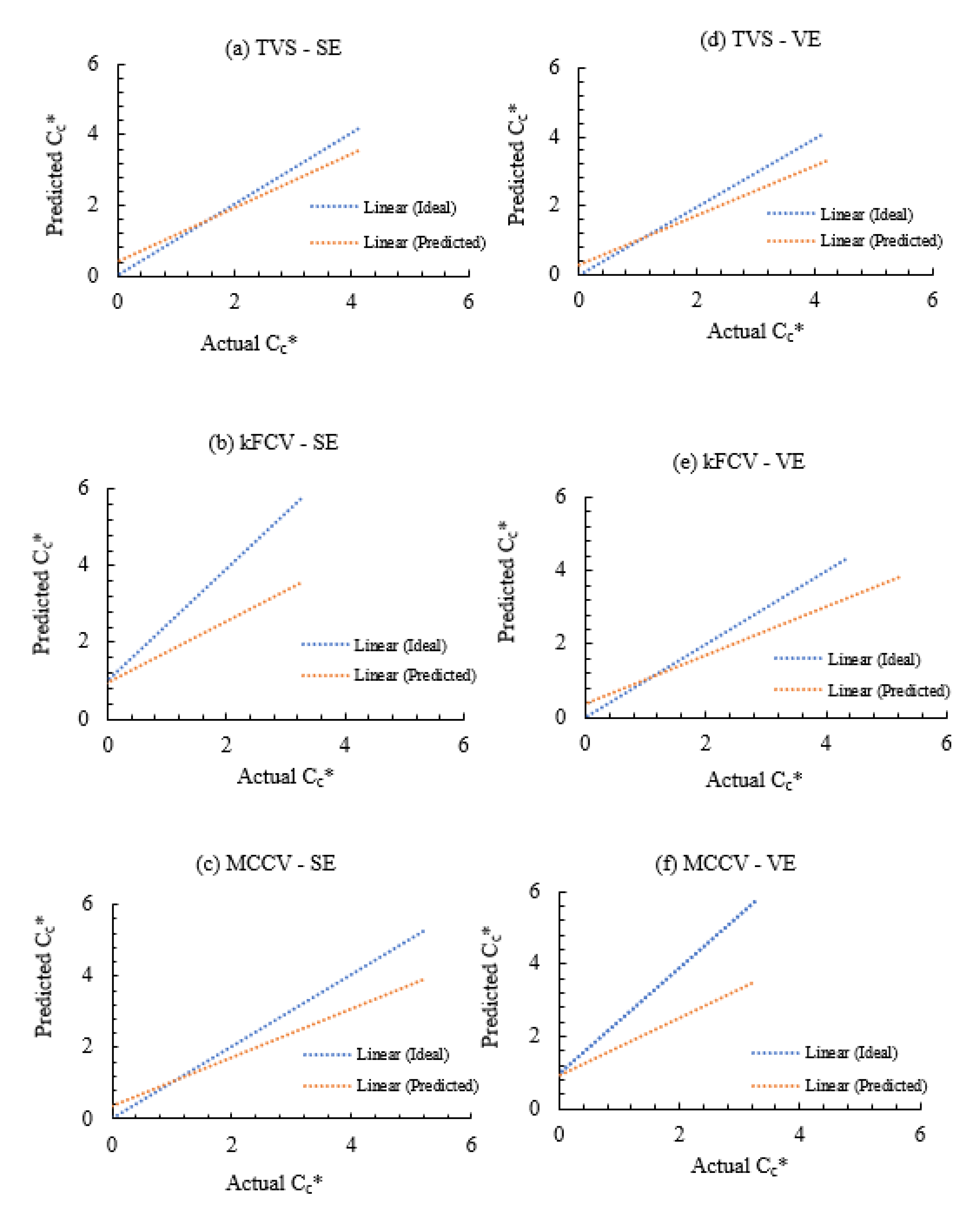
Table 5 and Figure 9 compare the performance of the hybrid meta-heuristic ensemble models across 3 cross validation methods. At first glance, it is observed that the method relying on the TVS seems to generally produce the highest values of R2 (with corresponding lower RMSE and MAE scores) from Table 5. This phenomenon is also demonstrated by the less degree of deviation of the predicted curve from the ideal line in Figure 9. On the other hand, the iterative method of training, testing, and validation for which kFCV and MCCV depend, tend to produce slightly lowers values of R2 compared to the TVS method. As mentioned previously, both kFCV and MCCV are used to improve the prediction of ML regression analyses while also serving as fine-tuning mechanisms to the TVS technique. Hence, the modelling with training and testing carried out using TVS when compared to kFCV and MCCV techniques seems to now indicate slight overfitting. Nonetheless, from Table 5 it is observed that the MCCV method does generally provide slightly much better accuracy than its kFCV counterpart. When also comparing between models, the prediction offered by the meta-ensembles using MCCV as a technique of cross validation, can be said to be more accurate than those of the stand-alone and tree ensembles which rely on the TVS method (Table 4). Although, when considered in terms of their Bias-Variance trade-offs, the MCCV is mostly deemed as having greater biases than the kFCV but with the former seeming to provide slightly more confidence in ML predictions given that it is more repeatable than the later due to its capacity to provide results with lower degrees of variance. Besides being characteristically prone to giving results with high variance, one other reason for KFCV’s poor performance is attributable to the number of its partitioning being limited by the number of folds used. However, a much closer examination of Table 5 indicates that ML testing and validation relying on a smaller number of folds (for both MCCV and kFCV) does marginally produce more accuracy.
It is important to bear in mind that depending on the situation, or the regression problem faced with, both MCCV and kFCV have been reported in the past as being able to provide better predictions than TVS. Nevertheless, within the context of this study, it is seen that the reverse seems to be the case. Again, judging from the method of cross validation used, model combination through voting does outperforms that done by stacking as Figure 9 indicates.

4.2.2. Model Residuals

Plot of the residuals of prediction does provide a means of validating ML models. By using residual plots, the observed errors of the best performing meta-heuristic models are assessed to ensure they are consistent with their corresponding stochastic errors (i.e., their randomness and unpredictability). Adopting this procedure is very necessary in this study given that none of the models used herein was able to produce 100% accuracy hence, these models could be regarded as inherently possessing some slight degree of errors. Another reason for using the residual plot is to assess the claims made of supposed overfitting in using the TVS validation methods and to evaluate the closeness of prediction when utilising both iterative cross validation methods—kFCV and MCCV.
A good model must always show independence of the residuals by having random errors left when learning the dataset. Figure 10 compares the independence of the errors of the meta-heuristic models across the validation methods. It is very interesting to observe that the TVS method does show a less independence of the stochastic errors even though ML dataset training relying on it showed earlier that its performance in terms of the statistical measures was the highest. However, as indicated in Figure 10, the data points are less symmetric about the origin while there is a corresponding high density of points and some measures of trending around the zero line. Moreover, there appears to be a pattern of distribution that is linear along the horizontal axis. This is indeed a confirmation of the less accuracy of the models’ prediction due to overfitting, when using the TVS method for training and testing of the dataset in this research. This also means that the models could not capture completely, the predictive information presented by the data hence, the reason there is a seepage of the data into the residuals.
Figure 10 also shows that the residuals of ML prediction given by the models with cross validation performed using both kFCV and MCCV techniques are quite independent. As could be observed, there are no forms of trending of the data points around the origin rather, there is much scatter and disordered patterns. Nevertheless, Figure 10 shows that that ML prediction of intrinsic compressibility with the cross validation carried out by using MCCV, provides the most accuracy given the symmetric and random distribution of residuals (no observable trends) about the origin for both voting and stacking models. Again, this diagnostic test has further validated the training, testing and validation of the meta-heuristic models performed using the MCCV as the best technique at least within the confines of this study.

4.2.3. Distribution of Residuals

Normal frequency distribution of the residuals does provide another ground for which a ML model effectiveness and authenticity can be assessed. Figure 11 indicates the normal distribution and histogram of the meta-heuristic models under three validation methods. Notice how both the models trained and validated by TVS and kFCV tend to be biased towards predicting values that are higher and lower, respectively, than the actual values of intrinsic compression index thus confirming their behaviour as demonstrated previously by their residual plots. On the other hand, ML prediction carried out with the models trained and validated using MCCV shows a much-balanced distribution as shown by the curve and indicating much better prediction. The corresponding histograms are also used to validate the accuracy of ML prediction. In this case, a very good model will tend to have its residuals peaking at zero but with few of the stochastic errors at its extremes while a low performing model will have its residual distribution spreading out but with fewer errors around zero. Using this theory, it could be observed that the best performing meta-ensemble models do have their training and validation done by adopting the MCCV method. It should also be mentioned that the voting technique across the three cross validations tend to slightly perform better than the technique of voting in general.

4.3. ML Classification

Different types of soils have been used for ML prediction from the forgoing. Hence, machine learning classification shall be applied as another form of diagnostic test in the forecast to ensure that the algorithms used properly learnt the different soil types and as such able to discriminate between each of the soil categories. By relying on their plasticity properties, this study utilises three different classes of soils defined according to the unified soil classification system (USCS) in the ML prediction. Hence, for the type of ML classification problem considered herein, the multiclass elements of the meta-models are used to predict the soil categories. The distribution of the soil classes in the dataset was given previously in Figure 3.

4.3.1. Receiver Operating Characteristic Curve (ROC) and Area under Curve (AUC)

To depict how well the meta-models are able to predict the probability of intrinsic compression index belonging to the different soil classes across some decision thresholds, the AUC-ROC are used. ROC plots the true positive rate (TPR) or sensitivity against false positive rate (FPR) or one less specificity given under various thresholds therefore separating “noise” from “signals” (Figure 12). Higher values on the horizontal axis, indicates higher number of the false positives compared to the true negatives. On the other hand, higher values on the vertical axis, indicate a higher number of true positives compared to false negatives. Hence, balancing between false positive and false negatives remains the choice of a chosen threshold. Meanwhile, AUC measures the actual capability of a model to differentiate between class labels. Hence, the higher the larger of AUC, the better the classifier at being able to distinguish between the positive and negative classes. When AUC equals 1, it therefore means that the model has been able to perfectly distinguish between the classes. However, a zero value would mean that the model has predicted all the positives as negatives and all the negatives as positives. When AUC is between 0.5 and 1, it means there is a higher chance that the model is capable of detecting more numbers of true positives and negatives than false negatives and positives. If AUC is exactly 0.5, then it means that the classifier is not able to differentiate between classes, in which case, it is just predicting constant or random class.
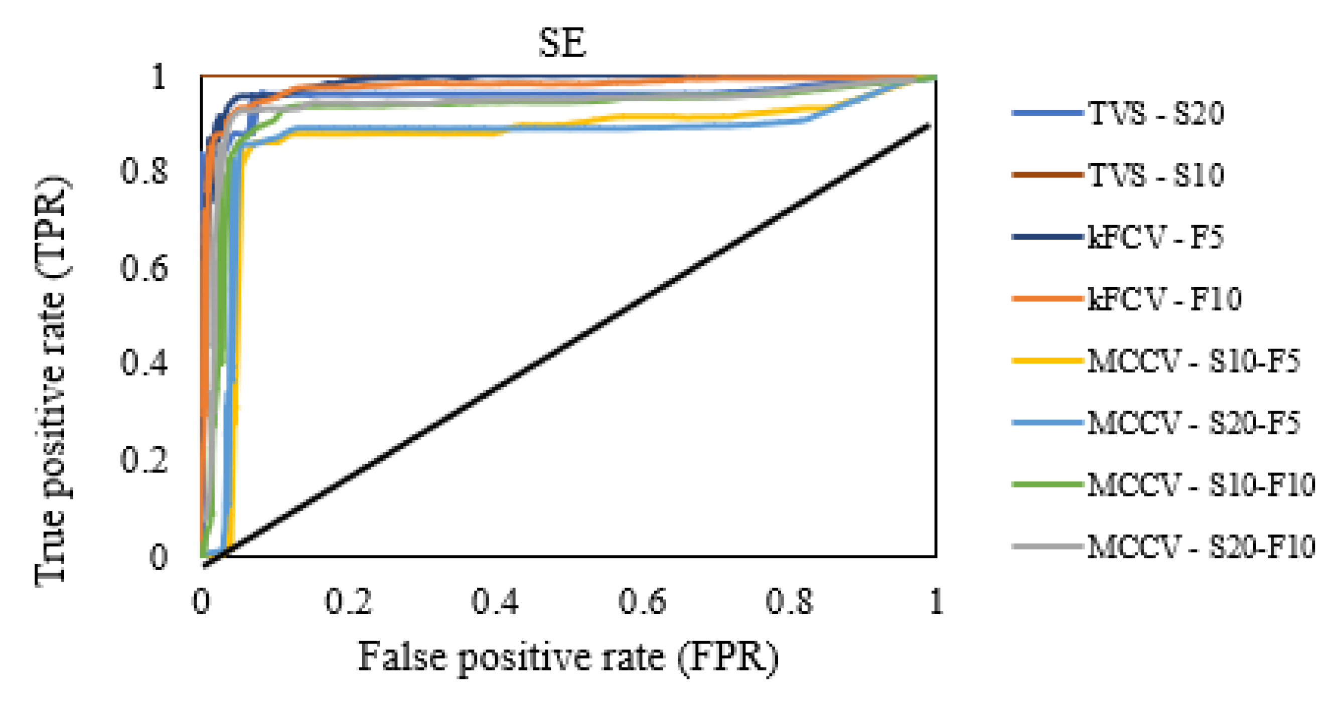
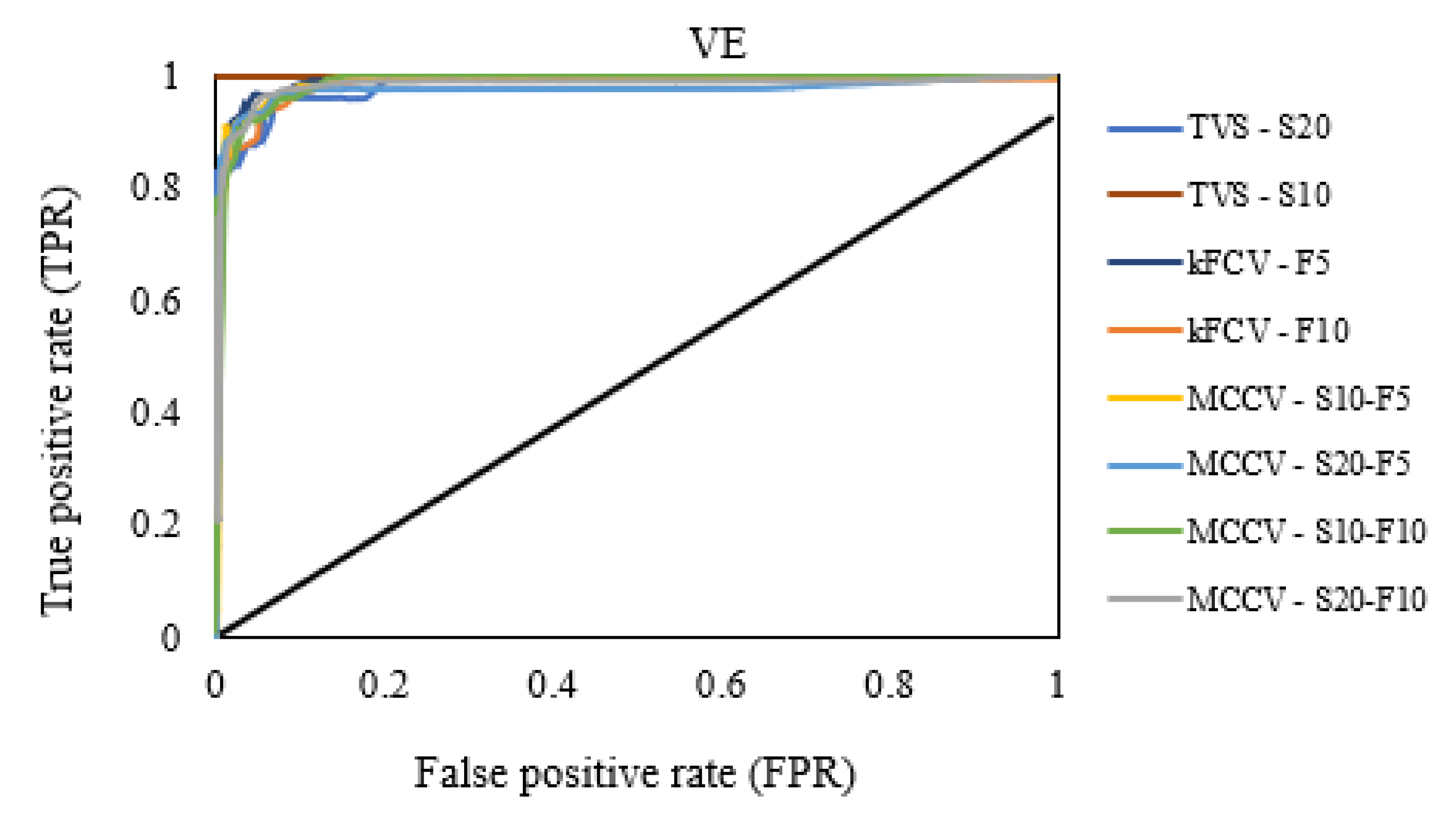
It could be observed from the ROC (Figure 13 and Figure 14) that the meta-ensembles all demonstrate the ability to discriminate between positive and negative classes. This also means that using the meta-ensembles in the multinomial class prediction has enabled a reduction in both type 1 and 2 prediction errors.
The dataset training and testing performed using the TVS appears to show perfect classification with an alignment of ROC with the top horizontal and left vertical axes. This again indicates an overfitting of the dataset given that the application of iterative cross validation techniques (kFCV and MCCV) results in slightly lower sensitivity compared to the TVS method. A closer examination of the corresponding Table 6 and Table 7 for both voting and stacking methods of model aggregation indicates that ML training and validation done by utilising the kFCV has the most sensitivity in distinguishing between the soil categories but with the 5-fold validation case having the highest overall AUC.
Further analysis of sensitivity as given by Table 8 indicates that the kFCV method has the best accuracy, recall rate and precision. When compared with the TVS method (with 20% of the dataset) originally used for testing of the algorithm, it could be observed that when using 5-fold cross validation multiclass predictions are higher by approximately 10–25% in terms of accuracy, rate of recall and precision. It is also interesting to observe that the kFCV method does also performs slightly better than MCCV on a multiclass problem such as that considered in this research. In this case, the disadvantage of using MCCV seems to weigh more heavily on multiclass prediction than on non-linear regression.
Table 8 also indicate that the assignment of uniform weights to cater for any under-represented class instances does clearly improves the individual multiclass accuracy compared to the overall accuracy metric. Further, it is also worth noting that the averaging of each class instances (i.e., micro-averaging), presents higher scores compared to the averaging that considers all equal class instances (i.e., macro-averaging) with respect to the most frequently occurring labels. Overall, by comparing the precision scores and recall rates, using micro-averaging does provide a higher sensitivity and thus better performance. However, it is needful to state that the application of the micro-averaging technique should be approached with care because unlike macro-averaging, it may not be suitable when dealing with an imbalanced class distribution given it does not average over larger group or class instances.
Generally, within the method of model aggregation used, it could also be observed that the voting method (VE) seems to generally perform better than its stacking counterpart across the validation methods used.

4.3.2. Comparing between Meta-Heuristic Ensembles and Traditional Classifiers

The superior performance of the meta-ensemble models (VE and SE) on the multiclass prediction of intrinsic compressibility of soils can be further validated by comparing them to other traditional ML multinomial classifiers namely, artificial neural networks (ANN), logistic regressor (LR), boosted decision trees BDT) and random decision forest (RDF). The sensitivity scores of the multiclass classification given in Table 9 indicates that both the stand-alone and tree-ensemble traditional ML classifiers do have the capability of distinguishing between soil plasticity categories just like the meta-heuristic ensemble models. Notwithstanding, among the traditional classifiers, the tree ensembles have clearly outperformed the stand-alone algorithms. ML prediction given by ANN is generally the least accurate as could be observed from Table 9. Some of the elements of the structure and architectural make-up of neural networks that do sometimes contribute to its poor performance, especially when applied in ML prediction problems such as those considered in this study, were stated previously in the regression prediction. Nevertheless, it is quite apt to add that the stand-alone models (ANN and LR) are in many respects quite similar given their common roots in statistics. However, the functional form of expression used as indicated in their mathematical equations stated above is what differentiates these classifiers. That which is used in LR is parametric whereas the ANN operates semi- or non-parametric functions. This is a very important distinction because most of the contributions given by parameters of an LR can be sufficiently interpreted whereas, as stated previously in the discussion of ML regression, those of ANN whose contributions are from the weights and biases may not be easily interpreted. On the other hand, the relatively high prediction accuracy of the tree-based classifiers is partly because their behaviour in learning is often suggested by a prior set of rules and hence, they are referred to as ‘white-boxes’ as compared to the neural networks. Hence, they tend to predict outcomes of classifications by continually splitting their inputs based on a set of criteria which then leads to a maximisation of the separation between the dataset and a decrease in entropy. The tree-based classifiers do have their setbacks hence, an aggregation of models into multiple classifiers carried out by stacking or by voting does further increase the accuracy of prediction as seen in Table 9 with the dataset trained, tested, and validated by the kFCV method.

4.3.3. Feature Importance

Indicators of the importance of independent features in ML prediction can also give an insight into the data used in the modelling as well as allow for an improvement of the efficacies of the models adopted. The relative significance and usefulness of the input variables used in the predictions of target features are depicted in Figure 15 for both the regression and multiclass classification ML predictions. The effect of each individual independent variables is herein assessed using the best prediction models. In terms of ML modelling and prediction of the intrinsic compressibility index of soils, it is clearly observed from Figure 15a that the feature of importance in this regard is the ratio of voids at 100 kPa of applied pressure. This is hardly surprising given the direct bearing of this measure quantity on C*c as previously demonstrated in the void index relationship. Among the other variables of indirect importance, the liquid limit including its corresponding void ratio prove to be the next most useful features in the forecast of C*c. It is very imperative to bear in mind that several strong linear relationships exist between the Atterberg limits and C*c as suggested by previously mentioned studies. On the other hand, when used for the first time in the prediction of C*c, the specific gravity or the texture element seems to bear the least influence at least within the remit of this research.
In terms of multiclass classification and when the average of the absolute class weights of the variables are considered, Figure 15b indicates that the Atterberg limits of the soils are the most significant factors in the determination of soil classes with the plasticity index wielding or having the highest numerical importance. This is a confirmation of the established research and theory that uses mostly the soil plasticity index for the direct and indirect determination of soil classes especially if the classification is carried out based on a standard provided by the unified soil classification system (USCS). By virtue of individual class vectors, the Atterberg limits features of the soils do generally seem to carry the most influence on the multiclass prediction of the soil categories as observed in Figure 15c. It is also interesting to note the individual importance of the ratio of voids at PI on the prediction of the relatively least plastic soils when compared to the actual Atterberg limits (both PI and LL). Again, as could be observed, the soil textural characteristics does not seem to be a lot useful in the prediction of the soil classes not to mention the derived features C*c.

5. Study Significance and Implementation

The significance of machine learning to geotechnical engineering design cannot be over- emphasized. The concept of artificial intelligence as applied in this study to predict the intrinsic compressibility of soils can save time and cost during the initial planning and design stages of soil investigation. For example, various tedious laboratory experimentation and time consuming trials that also involve the determination of influencial factors on soil instrinsic compressibility can be circumvented by adopting the methods carrried out in this reserach. However, in order to practically apply the best performing algorithms from this study, it is recommended that the background coding and scripting be persisted and deployed on any organisation’s computing resource and training or testing performed on new datasets of intrinsic compressibility of soils.

6. Conclusions

This study has used the machine learning (ML) approach to intelligently model the intrinsic compressibility index of soils by adopting non-parametric tree-based ensemble learners and meta-heuristic ensembles. Predictions using traditional stand-alone algorithms were also performed and compared with those of the ensemble learners. ML multiclass or multinomial classification was also applied to examine the ability of the classifiers to adequately learn between the soil types and by so doing distinguish between positive and negative classes. The following are the main conclusions from this study:
  • Among the traditional stand-alone ML regression models, BLR did produce the least accuracy of prediction of intrinsic compressibility index of soil when compared to REG and ANN. Although, a general consideration of the stand-alone ensembles such as REG and BLR would suggest their inability to implicitly detect the complexities of variable combinations due to their basic underlying assumption of linearity.
  • The tree ensembles (RDF and BDT) did generally outperform the stand-alone models with the RDF model having an R2 of 0.86 and RMSE of 0.48 and the BDT model producing and an R2 of 0.822 and RMSE of 0.53. The techniques of ‘bagging’ or ‘bootstrapping’ inherent in these tree-ensembles certainly enhanced their accuracy in that respect.
  • The technique of ensemble averaging with a meta-heuristic combination of models’ hyperparameters through voting and stacking gave the best overall performance in the prediction of the intrinsic compressibility index of soils with an average R2 of 0.9 and RMSE of 0.34.
  • Sensitive analysis and diagnostic tests used to examine the procedure and outcome of dataset training, testing and validation showed the Monte Carlo method of cross validation as giving the best results for ML prediction.
  • An analysis of the features with direct influence on the ML prediction revealed that the void ratio determined at effective stress of 100 kPa had the most significance followed by soil’s Atterberg limits while specific gravity was the variable of least importance in the forecast of intrinsic compressibility index of soils C*c.

Author Contributions

Conceptualisation, E.U.E. and S.J.A.; methodology, E.U.E. and S.J.A.; validation, E.U.E. and S.J.A.; formal analysis, E.U.E. and S.J.A.; investigation, E.U.E. and S.J.A.; resources, S.J.A. and C.A.B.; data curation, E.U.E. and S.J.A.; writing—original draft preparation, E.U.E. and S.J.A.; writing—review and editing, E.U.E., S.J.A. and C.A.B.; visualisation, S.J.A. and C.A.B.; supervision, C.A.B.; project administration, C.A.B. All authors have read and agreed to the published version of the manuscript.

Funding

This research received no external funding.

Institutional Review Board Statement

Not applicable.

Informed Consent Statement

Not applicable.

Conflicts of Interest

The authors declare no conflict of interest.

References

  1. Gu, X.; Zhang, J.; Huang, X. DEM analysis of monotonic and cyclic behaviors of sand based on critical state soil mechanics framework. Comput. Geotech. 2020, 128, 103787. [Google Scholar] [CrossRef]
  2. Roscoe, K.H.; Schofield, A.N.; Wroth, C.P. On the Yielding of Soils. Geotechnique 1958, 8, 22–53. [Google Scholar] [CrossRef]
  3. Yang, J.; Li, X.S. State-Dependent Strength of Sands from the Perspective of Unified Modeling. J. Geotech. Geoenviron. Eng. 2004, 130, 186–198. [Google Scholar] [CrossRef] [Green Version]
  4. Feng, L.; Zhang, S.; Jin, Z.; Zhang, M.; Sun, P.; Jia, J.; Chu, G.; Hu, W. The critical mechanics of the initiation of loess flow failure and implications for landslides. Eng. Geol. 2021, 288, 106165. [Google Scholar] [CrossRef]
  5. Nguyen, H.B.K.; Rahman, M.; Fourie, A. The critical state behaviour of granular material in triaxial and direct simple shear condition: A DEM approach. Comput. Geotech. 2021, 138, 104325. [Google Scholar] [CrossRef]
  6. de Bono, J.P.; McDowell, G.R. Micro mechanics of the critical state line at high stresses. Comput. Geotech. 2018, 98, 181–188. [Google Scholar] [CrossRef]
  7. Burland, J.B. On the compressibility and shear strength of natural clays. Géotechnique 1990, 40, 329–378. [Google Scholar] [CrossRef]
  8. Cerato, A.; Lutenegger, A.J. Determining Intrinsic Compressibility of Fine-Grained Soils. J. Geotech. Geoenvironmental Eng. 2004, 130, 872–877. [Google Scholar] [CrossRef]
  9. Lee, C.; Hong, S.-J.; Kim, D.; Lee, W. Assessment of Compression Index of Busan and Incheon Clays with Sedimentation State. Mar. Georesources Geotechnol. 2015, 33, 23–32. [Google Scholar] [CrossRef]
  10. Tsuchida, T. e–logσv′ relationship for marine clays considering initial water content to evaluate soil structure. Mar. Georesources Geotechnol. 2017, 35, 104–119. [Google Scholar] [CrossRef]
  11. Zeng, L.-L.; Hong, Z.-S.; Cui, Y.-J. Determining the virgin compression lines of reconstituted clays at different initial water contents. Can. Geotech. J. 2015, 52, 1408–1415. [Google Scholar] [CrossRef]
  12. Al Haj, K.; Standing, J. Mechanical properties of two expansive clay soils from Sudan. Geotechnique 2015, 65, 258–273. [Google Scholar] [CrossRef]
  13. Hong, Z.S.; Zeng, L.L.; Cui, Y.J.; Cai, Y.Q.; Lin, C. Compression Behaviour of Natural and Reconstituted Clays. Geotechnique 2012, 62, 291–301. [Google Scholar] [CrossRef] [Green Version]
  14. Xu, G.-Z.; Yin, J. Compression Behavior of Secondary Clay Minerals at High Initial Water Contents. Mar. Georesources Geotechnol. 2016, 34, 721–728. [Google Scholar] [CrossRef]
  15. Habibbeygi, F. Intrinsic compression characteristics of an expansive clay from western australia. Int. J. Geomate 2017, 12, 140–147. [Google Scholar] [CrossRef]
  16. Habibbeygi, F.; Nikraz, H.; Koul, B.K. Regression models for intrinsic constants of reconstituted clays. Cogent Geosci. 2018, 4, 1546978. [Google Scholar] [CrossRef]
  17. Kootahi, K.; Moradi, G. Evaluation of compression index of marine fine-grained soils by the use of index tests. Mar. Georesources Geotechnol. 2017, 35, 548–570. [Google Scholar] [CrossRef]
  18. Cerato, A.B. Influence of Specific Surface Area on Geotechnical Characteristics of Fine-Grained Soils; University of Massachusetts: Amherst, MA, USA, 2001. [Google Scholar]
  19. Onofrio, A.; Santucci de Magistris, F.; Olivares, L. Influence of Soil Structure on the Behavior of Two Natural Stiff Clays in the Pre-Failure Range. In Proceedings of the 2nd International Symposium on the Geotechnics of Hard Soils-Soft Rocks, Naples, Italy, 12–14 October 1998; pp. 497–505. [Google Scholar]
  20. Yagi, N.; Yatabe, R.; Mukaitani, M. Compressive Characteristics of Cohesive Soils. In Proceedings of the International Symposium on Compression and Consolidation of Clayey Soils, IS-Hiroshima, Hiroshima, Japan, 10–12 May 1995; Hiroshi, Y., Osamu, K., Eds.; A.A. Balkema: Rotterdam, The Netherlands, 1995; pp. 221–226. [Google Scholar]
  21. Gori, U.; Polidori, E.; Tonelli, G. The One-Dimensional Consolidation Effect on the Slightly Sensitive Soils. In Proceedings of the International Symposium on Compression and Consolidation of Clayey Soils, IS-Hiroshima, Hiroshima, Japan, 10–12 May 1995; pp. 49–55. [Google Scholar]
  22. Yamadera, A.; Miura, N.; Hino, T. Microscopic Consideration on Compression and Rebound Behaviors of Ariake Clay. In Proceedings of the International Symposium, Bothkennar, Drammen, Quebec & Ariake Clays, Yokosuka, Japan, 26–28 February 1997; pp. 175–184. [Google Scholar]
  23. Nagaraj, T.S.; Srinivasa, B.R.; Murthy, S. A critical reappraisal of compression index equations. Geotechnique 1986, 36, 27–32. [Google Scholar] [CrossRef]
  24. Nagaraj, T.S.; Pandian, N.S.; Raju, N. Stress state-permeability fine-grained. Geotechnique 1993, 43, 333–336. [Google Scholar] [CrossRef]
  25. Sridharan, A.; Nagaraj, H.B. Compressibility behaviour of remoulded, fine-grained soils and correlation with index properties. Can. Geotech. J. 2000, 37, 712–722. [Google Scholar] [CrossRef]
  26. Meriggi, R.; Paronuzzi, P.; Simeoni, L. Engineering geology characterization of lacustrine overconsolidated clays in an alpine area of Italy. Can. Geotech. J. 2000, 37, 1241–1251. [Google Scholar] [CrossRef]
  27. Skempton, A.W.; Jones, O.T. Notes on the compressibility of clays. Q. J. Geol. Soc. 1944, 100, 119–135. [Google Scholar] [CrossRef]
  28. Youssef, M.S.; Ramli, A.H.; Demery, M.E. Relationships Between Shear Strength, Consolidation, Liquid Limit, and Plastic Limit for Remoulded Clays. In Proceedings of the Sixth International Conference on Soil Mechanics and Foundation Engineering, Montreal, QC, Canada, 8–15 September 1965; pp. 126–129. [Google Scholar]
  29. Quigley, R.M.; Thompson, C.D. The Fabric of Anisotropically Consolidated Sensitive Marine Clay. Can. Geotech. J. 1966, 3, 61–73. [Google Scholar] [CrossRef]
  30. Akagi, H.; Komiya, K. Constant Rate of Strain Consolidation Properties of Clayey Soil at High Temperature. Volume 1 of Compression and Consolidation of Clayey Soils. In Proceedings of the International Symposium on Compression and Con-solidation of Clayey Soils, IS-Hiroshima, Hiroshima, Japan, 10–12 May 1995; pp. 3–8. [Google Scholar]
  31. Raymond, G.P. Laboratory Consolidation of Some Normally Consolidated Soils. Can. Geotech. J. 1966, 3, 217–234. [Google Scholar] [CrossRef]
  32. Locat, J.; Lefebure, G. The Compressibility and Sensitivity of an Artificially Sedimented Clay Soil: The Grande-Baleine Marine Clay. In Proceedings of the 2nd Canadian Conference on Marine Geotechnical Engineering, Halifax, NS, Canada, 1–3 June 1982. [Google Scholar]
  33. Jardine, R.J. Investigations of Pile-Soil Behaviour, with Special Reference to the Foundations of Offshore Structures. PhD thesis, The University of London, London, UK, 1985. [Google Scholar]
  34. Templeton, G.F. A Two-Step Approach for Transforming Continuous Variables to Normal: Implications and Recommendations for IS Research. Commun. Assoc. Inf. Syst. 2011, 28, 41–58. [Google Scholar] [CrossRef] [Green Version]
  35. Yu, H.-F.; Huang, F.-L.; Lin, C.-J. Dual coordinate descent methods for logistic regression and maximum entropy models. Mach. Learn. 2011, 85, 41–75. [Google Scholar] [CrossRef] [Green Version]
  36. Huang, F.-L.; Hsieh, C.-J.; Chang, K.-W.; Lin, C.-J. Iterative scaling and coordinate descent methods for maximum entropy. J. Mach. Learn. Res. 2010, 11, 815–848. [Google Scholar] [CrossRef]
  37. Galwey, N. Introduction to Mixed Modelling: Beyond Regression and Analysis of Variance, 2nd ed.; Wiley: Chichester, UK, 2014. [Google Scholar]
  38. Chatterjee, S.; Hadi, A. Regression Analysis by Example, 5th ed.; Wiley: Hoboken, NJ, USA, 2012. [Google Scholar]
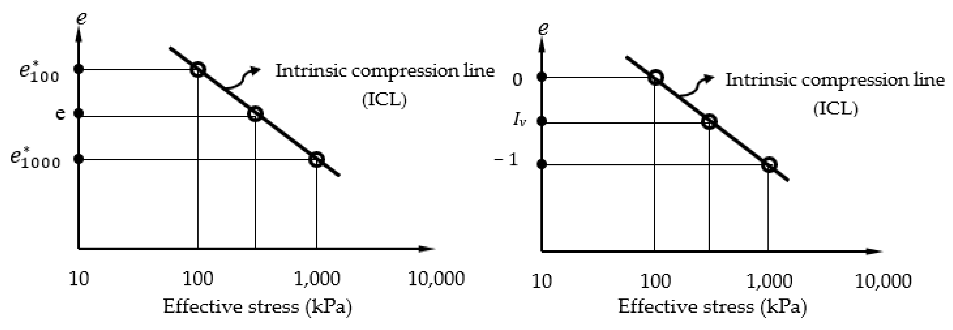
Figure 1. Plots of void ratio vs. effective stress showing intrinsic constants, ICL and void index.
Applsci 12 09940 g001
Figure 2. Distribution of intrinsic compressibility index.
Applsci 12 09940 g002
Figure 3. Distribution of ML features. (a) specific gravity; (b) Plastic limit; (c) Void ratio at LL; (d) Void ratio at 100 kPa stress; (e) Liquid limit; (f) Plasticity index; (g) Void ratio at PL; (h) Soil class.
Applsci 12 09940 g003
Figure 4. Typical decision trees.
Applsci 12 09940 g004
Figure 5. Typical structure of voting ensemble.
Applsci 12 09940 g005
Figure 6. Typical structure of stacking ensemble.
Applsci 12 09940 g006
Figure 7. Architecture of artificial neural network.
Applsci 12 09940 g007
Figure 8. Summary of ML methodology.
Applsci 12 09940 g008
Figure 9. Ideal v actual intrinsic compressibility index.
Applsci 12 09940 g009
Figure 10. Residual plots.
Applsci 12 09940 g010
Figure 11. Distribution of residuals.
Applsci 12 09940 g011
Figure 12. Typical ROC plots.
Applsci 12 09940 g012
Figure 13. ROC plot for SE model.
Applsci 12 09940 g013
Figure 14. ROC plot for VE model.
Applsci 12 09940 g014
Figure 15. ML Feature importance.
Applsci 12 09940 g015
Table 1. Statistics of intrinsic compressibility index ( C c * ).
MeanStandard ErrorStandard DeviationKurtosisSkewnessMin.Max.Range
0.7892440.1247821.36121−0.09140.1234570.088.58.42
Table 2. Statistics of explanatory features.
StatisticGLLPLPI e L e p e 100 *
Mean2.7187.6231.1156.502.370.841.51
Standard Error0.018.3751.1967.820.220.030.10
Standard Deviation0.1091.3613.0585.252.430.361.08
Kurtosis0.8613.939.1516.1112.9411.599.53
Skewness−0.53.602.053.943.492.362.78
Range0.565389650313.682.756.65
Min.2.37221250.590.310.45
Max.2.9356010850814.273.067.10
Table 3. Models’ optimised parameter settings.
Stand-Alone Algorithms
ParameterOption/value
REGRegularisation wt. (L2)0.001
MethodOrdinary least squares (OLS)
LROptimisation tolerance1 × 10−7
Regularisation wt. (L1 & L2)1.00
BLRRegularisation wt. (L2)1.00
ANNNormalisermin-max
No. of hidden nodes100.00
No. of iterative learning100.00
Hidden layer spec.Full connection
Tree-ensembles
ParameterOption/value
Boosted decision tree (BDT)Constructed trees100.00
Tree-forming training instances 10.00
Leaves/tree (max.)20.00
Random decision forest (RDF)Tree depth (max.)32.00
Constructed trees8.00
Method of resamplingBagging
Samples/leaf node (min.)1.00
Randomised splits/node128.00
Table 4. ML regression performance metrics.
ModelR2RMSEMAE
%%
REG0.670.730.54
ANN0.590.810.61
BLR0.191.141.02
BDT0.820.530.44
RDF0.860.480.38
SE0.930.340.29
VE0.930.330.26
Table 5. ML regression performance metrics by method of dataset testing and validation.
Model R2RMSEMAE
CV MethodSetNo. of Folds %%
TVS20-0.930.340.29
10-0.670.660.62
SEKFCV-50.880.440.33
-100.860.440.33
MCCV1050.890.400.31
2050.880.460.35
10100.880.430.34
20100.880.460.36
TVS10-0.910.340.29
20-0.930.330.26
VEKFCV-50.880.430.32
-100.860.430.32
MCCV1050.900.400.32
2050.880.450.35
10100.870.440.35
20100.880.460.36
Table 6. AUC metrics for SE model.
ModelCV MethodSetNo. of Folds AUC
MicroMacroWeighted
TVS20-0.9570.8690.975
TVS10-1.0001.0001.000
SEKFCV-50.9890.9820.992
KFCV -100.9820.9860.992
MCCV 1050.8610.8130.833
MCCV 2050.8900.8430.911
MCCV 10100.9230.8870.904
MCCV 20100.9460.9290.946
Table 7. AUC metrics for VE model.
ModelCV MethodSetNo. of Folds AUC
MicroMacroWeighted
TVS20-0.9860.9860.996
TVS10-1.0001.0001.000
VEKFCV-50.9920.9840.993
KFCV -100.9910.9960.998
MCCV 1050.9500.9640.973
MCCV 2050.9740.9690.984
MCCV 10100.9660.9760.979
MCCV 20100.9830.9820.990
Table 8. ML multinomial classification performance metrics.
ModelCV MethodSet (S)No. of Folds (F)AccuracyRecallPrecision
OverallWeightedMicroMacroWeightedMicroMacroWeighted
TVS20-0.8330.9380.8330.5630.8330.8330.5750.775
TVS10-1.0001.0001.0001.0001.0001.0001.0001.000
SEKFCV-50.9240.9720.9240.7580.9240.9240.7870.908
KFCV-100.9330.9640.9330.8560.9330.9330.8550.923
MCCV1050.8170.8560.8170.7560.8170.8170.7340.776
MCCV2050.8580.9110.8580.7460.8580.8580.7450.809
MCCV10100.8580.8930.8580.8050.8580.8580.7650.820
MCCV20100.9080.9460.9080.8060.9080.9080.8030.875
TVS20-0.8750.9570.8750.6250.8750.8750.6830.850
TVS10-1.0001.0001.0001.0001.0001.0001.0001.000
VEKFCV-50.9580.9820.9580.8560.9580.9580.8650.946
KFCV-100.9410.9750.9410.8610.9410.9410.8590.928
MCCV1050.9170.9360.9170.8650.9170.9170.8830.922
MCCV2050.9250.9690.9250.7960.9250.9250.8030.901
MCCV10100.9000.9350.9000.8240.9000.9000.8160.877
MCCV20100.9210.9640.9210.7810.9210.9210.7780.897
Table 9. Sensitivity metrics for traditional ML algorithms and meta-ensembles with dataset training and validation done under k-fold CV method.
ModelBDTRDFLRANNVESE
10 CV5 CV10 CV5 CV10 CV5 CV10 CV5 CV10 CV5 CV10 CV5 CV
Accuracy0.8980.9070.8980.8660.7470.7310.7210.6900.9410.9580.9330.924
Precision0.8690.8050.8360.7720.5310.5230.5230.4550.8590.8650.8560.787
Recall0.8780.8360.8420.7150.6340.5700.5850.5200.8610.8560.8560.758
Publisher’s Note: MDPI stays neutral with regard to jurisdictional claims in published maps and institutional affiliations.