Article

Enhancing Channelized Feature Interpretability Using Deep Learning Predictive Modeling

by
Salbiah Mad Sahad
1,2,*,
Nian Wei Tan
1,
Muhammad Sajid
1,
Ernest Austin Jones, Jr.
1 and
Abdul Halim Abdul Latiff
2
1
GeoImaging Technology, PETRONAS Research Sdn Bhd (PRSB), Lot 3288 & 3289, Off Jln Ayer Itam, Kawasan Institusi Bangi, Kajang 43000, Malaysia
2
Centre of Subsurface Imaging, Department of Geosciences, Universiti Teknologi PETRONAS, Seri Iskandar 32610, Malaysia
*
Author to whom correspondence should be addressed.
Appl. Sci. 2022, 12(18), 9032; https://doi.org/10.3390/app12189032
Submission received: 13 June 2022 / Revised: 12 August 2022 / Accepted: 15 August 2022 / Published: 8 September 2022
(This article belongs to the Special Issue Big Data and Machine Learning in Earth Sciences)

Abstract

:
Automating geobodies using insufficient labeled training data as input for structural prediction may result in missing important features and a possibility of overfitting, leading to low accuracy. We adopt a deep learning (DL) predictive modeling scheme to alleviate detection of channelized features based on classified seismic attributes (X) and different ground truth scenarios (y), to imitate actual human interpreters’ tasks. In this approach, diverse augmentation method was applied to increase the accuracy of the model after we were satisfied with the refined annotated ground truth dataset. We evaluated the effect of dropout as a training regularizer and facies’ spatial representation towards optimized prediction results, apart from conventional hyperparameter tuning. From our findings, increasing batch size helps speedup training speed and improve performance stability. Finally, we demonstrate that the designed Convolutional Neural Network (CNN) is capable of learning channelized variation from complex deepwater settings in a fluvial-dominated depositional environment while producing outstanding mean Intersection of Union (IoU) (95%) despite utilizing 6.4% from the overall dataset and avoiding overfitting possibilities.

1. Introduction

The essence of modern sedimentary basins highlights the elements of meandering channels and corresponding meandering belts. Identification of fluvial channels has been considered crucial and requires expert knowledge by looking into the factors controlling the sandstone body shape, dimensions, connectivity, and internal heterogeneity [1]. Conventional subsurface facies analysis for meandering fluvial channels was initially employed based on the characteristics of vertical profile (according to Walter’s law of facies succession) and morphology of the channels [2].
Since channels pose as an important hydrocarbon indicator for the clastic depositional environment, whether in exploration or development projects, the conventional method of detecting sand-filled geobodies, guided by multiple seismic attribute extraction, is considered exhaustive yet time-consuming, contrasting with the growing demand for higher-resolution yet higher-bandwidth seismic data. Although seismic attributes have the capability to enhance details leading to better geological and geophysical data, they also have the tendency to create new interpretational pitfalls. The growth of seismic attribute technology in accelerating the advancement of exploration and development started in the late 1960s, with identification of bright spots through seismic reflection traits [3]. Most positive curvatures were capable of illuminating crispier lineaments of meandering channels compared to coherence attributes [4]. Sweetness was proven as an important attribute for predicting net-to-gross ratio using semi-quantitative application for different superimposed channels [5]. In between the captured timeline, pattern recognition or neural network-based analysis on seismic attributes since the 1990s has gradually brought significant improvement in defining structures or depositional environments.
Conventional technology has emphasized the usage of seismic reflection patterns to predict depositional environment, structural deformation, and diagenetic alteration by constraining lithology and porosity information. Knowledge of and experience with seismic patterns or textures stored in the brain were applied by human interpreters to infer the possible geological setting using digital or analog data, combining geology, geophysics, and petrophysical disciplines [6]. Understanding the geomorphology of channels, specifically in clastic depositional environments, showcased the conventional application of multiple seismic attributes to extract information such as segments of channels, discontinuities, dip, and azimuth. With the advancement of neural network technology over the past twenty years, extracting continuous channel bodies based on the information of related seismic facies in the known settings, for instance, helps interpreters to accelerate their structural interpretation, and hence, mapping for challenging structures becomes easier for further analysis in reservoir characterization, inversion, geohazard avoidance, and many more applications.
We implement a deep learning (DL) predictive modeling scheme to improve channel interpretation by exploiting classified seismic attributes [7] as the input to infer quantitative property/structural information (Table 1) and 2D U-Net Network structure, due to its reliability and stable performance, with minimum time required for debugging. Different types of ground truth are attached to imitate the actual process used by human interpreters on synthetic and real field data. The term “Ground Truth” in deep learning has been defined as a conceptual term relative to the knowledge of truth concerning a specific question, with ideal expected results and statistical models or research hypotheses to be supported. By taking image segmentation challenges into seismic images perspectives, ground truth may specifically refer to pixel-based identification compared to the input data. In a supervised learning method, ground truth will be part of the training set to teach the neural network model to identify features and non-features. The algorithm measures its accuracy using an applied loss function and will be adjusted (between the input and the modeled) until errors have been minimized sufficiently.

1.1. SEG Advanced Modeling (SEAM) Dataset

To ensure the algorithms are robust and effective, we use the Society of Exploration Geophysicists (SEG) Advanced Modeling (SEAM) Phase 1 dataset [8] as the training data. Figure 1a shows a general overview of geological structures in the SEAM Reservoir Model, which consists of highly channelized complexes, sheet turbidites, and localized turbidite fans, with the red region marked as the training dataset. Three reservoir types representing local turbidite fans, widespread and superposed turbidite sheets with highly channelized complexes were developed, consist of various types of fluids (oil, gas, and brine). Seven localized turbidites were present in Pleistocene formation, while extensive sheet turbidites covered several stratigraphic horizons of Middle and Lower Miocene macro-layers. Full turbidite complexes with a pair of estimated 80 m-thick sub-sheets were parted by shale background layers with estimated channel width of 2 km in the same interval, with clear indication of en echelon structures, as depicted in Figure 1b. A section of volume of shale illustrates stratigraphic features from the Pleistocene to Cretaceous, highlighting the stacked channels in Upper Miocene. Superposed sixteen pairs of stacked channels with horizontal distance of 8 km are depicted in Figure 1c.

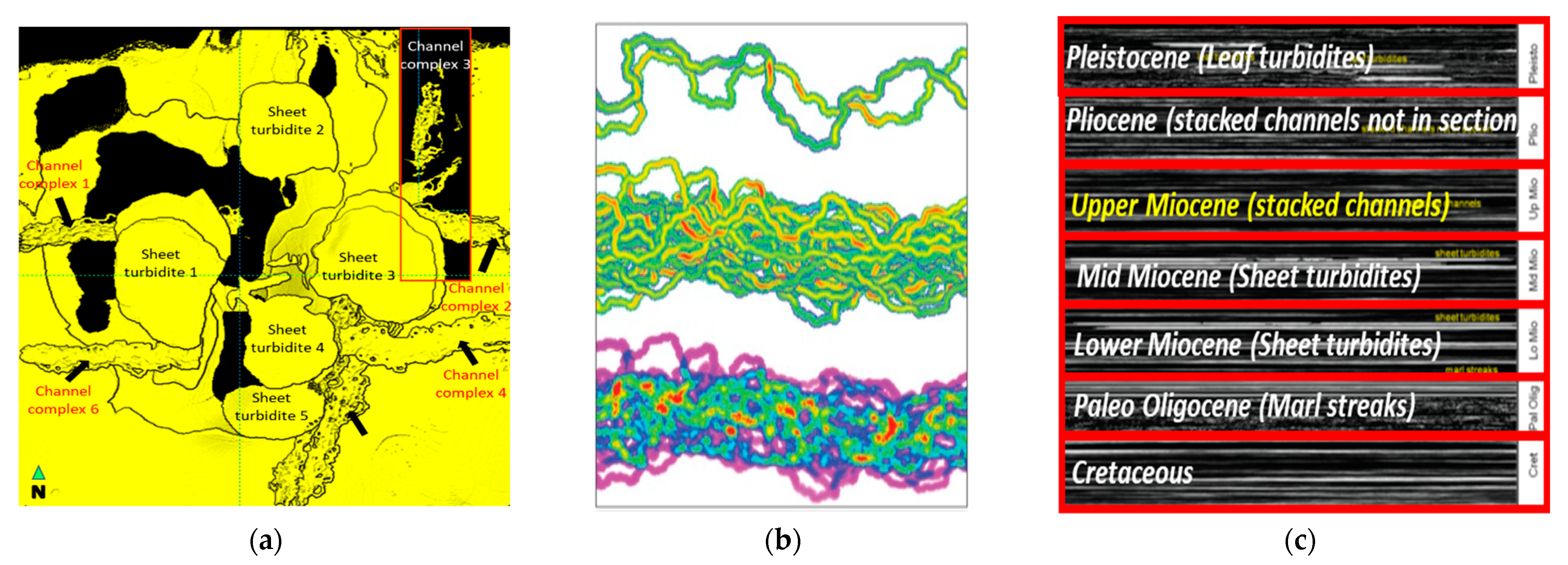
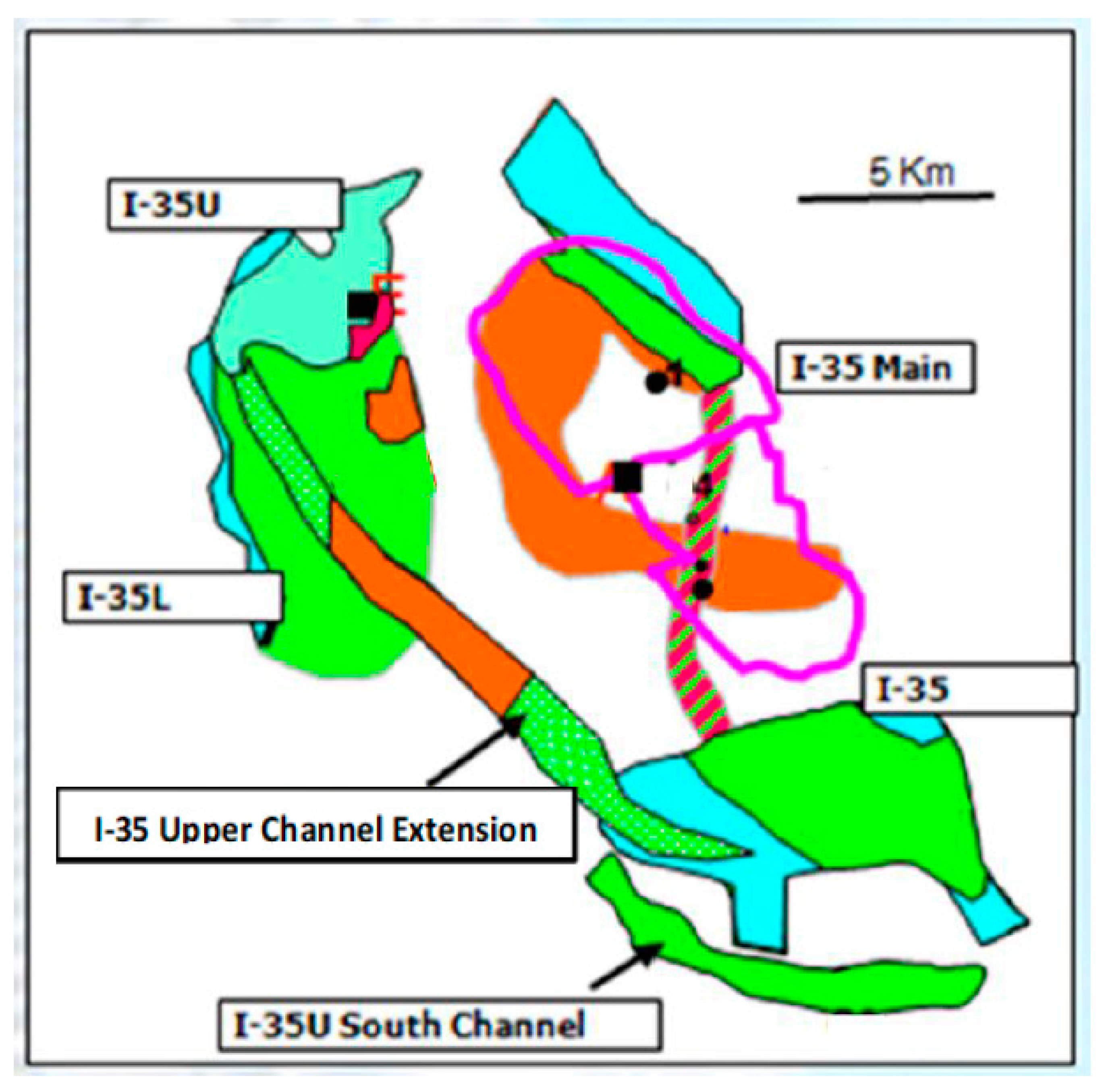
1.2. Geological Settings of A Field

The study was conducted in A Field, which can be described as anticline-elongated in the northwest–southeast direction with an average water depth of 69 m. The field measures 25,000 acres at the I and J Reservoir levels, with a column height of 100 m at the I-25 reservoir and nearly flat structure, with dip angle ranging from 1 to 3 degrees. The stratigraphy of the field is made up of interbedded sequences of sandstones, siltstone, and claystone with minor coal, which is deposited in fluvial, lacustrine, and marginal marine environments. It is divided into nine formation groups, namely, Groups M, L, K, J, I, H, F, A, and B (according to the lithostratigraphic scheme from Malay Basin Tertiary Sediments). Hydrocarbons are found in Groups M, L, K, J, and I of age Late Oligocene to Middle Miocene. However, the hydrocarbon only accumulates within Group I, J, and K Reservoirs. Group I Sandstone is 450 m thick. We elevate our scopes in I-35 Reservoir as it is the main oil-bearing reservoir in the A Field, which is well developed in the Main, West, and South areas (see Figure 2).

1.3. Overview of Neural Network-Based Technology

Early neural network approaches in seismic pattern recognition [9] suggested multiple blending of morphologic and curvature attributes to delineate the geomorphology of different features, and highlighted Sobel filter applications in enhancing discontinuity edges, resulting in focused images of specific geological interests. The concept of training features with multiple neural network architectures using gradient descent has been introduced by [10] to reduce the cost function. Under a deep learning platform, fewer hand-engineered data were required with a Convolutional Neural Network (ConvNet or CNN) for training and classifying images or patterns in multiple arrays [11]. End-to-end automated network architecture to predict salt bodies was developed by combining SegNet and a statistical approach [12]. The proposed method solely relied on interactive salt body labeling tools and a limited number of training data. Regardless, accurate prediction on salt bodies in slices, inlines, and crossline sections were observed in the blind dataset, proving faster and quantitatively adding value in the latest automated structural interpretation [13]. The concept of CNN has been shifted by [14] into classified seismic attributes to interpret salt boundaries and compared results with the conventional interpretation. Insufficient labeled geophysical data for supervised classification challenges has been addressed by [15] leading to the possibility of overtraining for small-scale labeled datasets and unstable predictions for unlabeled datasets. Convolutional Neural Network (CNN) and VGG-16 provided solid accuracies and fast transfer learning interpreting different seismic facies patterns to identify salt bodies in F3 Field, The Netherlands as demonstrated by [16].

1.4. Application of Neural Network in Geological Feature Identification

Subsurface modeling and seismic interpretation technology have rapidly evolved over the past twenty years in order to obtain the most accurate extraction of such features as unconformities, channels, faults, carbonate (specifically karst-related), and even to delineate salt bodies. The applicability of approximation theorem to mimic a non-linear operator for a deep neural network-based platform was introduced by [17]. Conventional Machine Learning (ML) method to build multi-layer perceptron (MLP) and K-means clustering to aid seismic feature classification [18]. A combination of extensive image processing and ML methods by emphasizing a structural tracking algorithm was introduced by [19] to enhance salt domes and faults, with detailed reservoir characterization. Reassuring approach inferring 3D labeled synthetics for channelized body prediction in 3D field datasets utilizing minimum training data being fed into the neural network was demonstrated by [20]. Salt boundary estimation for velocity model building and detailed understanding on salt tectonics has been successful in an experiment using U-Net whereby the proposed method replaced the encoder-decoder network architecture with 3D operators to automate salt probability volumes [21].

2. Methodology

Figure 3 encapsulates an integrated framework implementing an end-to-end supervised learning pipeline and comprises the following steps:
(a)
We extract sixteen types of seismic attributes (Figure 4) and normalize the dataset into Gaussian scale during Exploratory Data Analysis (EDA).
(b)
Preparing the label data. We use two ground truth scenarios to fit into the requirements of the data availability from an expert’s perspectives.

2.1. Blob-Based Method

Building a 3D geological model is the most common approach for defining ideal subsurface information as the ground truth. Detailed reference and understanding of the depositional system help to refine the quality of the label dataset. The SEAM Phase 1 dataset with a size of 1024 (inlines) × 256 (crosslines) and depth ranging from 6180 to 7180 m was chosen as the study area. Using the volume of a shale cube, we extract the amplitude values for three different facies, namely, channel, salt bodies, and background using calculator function in Petrel, to generate a new seismic volume and convert it into numerical Python format. Next, we re-classify the facies classes into class 0 (represents background data), class 1 (represents channel), and class 2, referring to salt bodies in Python. The next step is integrating the label with sixteen seismic attributes for binary classification, embedded in the same Python code.

2.2. Python-Based Labeling Tool

The essence of supervised learning methods highlights the capability of neural network algorithms to generalize training dataset in the unfamiliar scenarios and “trained” DL inferences to make accurate predictions [22]. In preparation for these, the 3D seismic data cube was 2 millisecond-sampled with a size of 1024 × 256 (inlines, crosslines) and 64 layers of data were annotated in the z-direction. Figure 5 shows how fluvial facies are labeled in I-35 Lower Reservoir, in A Field, and categorized according to specific classes, as indicated in Table 2. Reservoir field issues, reservoir geometry, and interpreted depositional environments were considered to further understand the regional geology of Malay Basin. To ensure the accuracy of the labeling process, we executed Log Pattern Analysis from twelve nearby wells including one cored well to the annotated data layers. Using commercial packages, interpreters need to validate the quality of the labeled features and certify that no empty spaces were found to avoid misleading in classification by the neural network later.
(c)
We define the network architectures using Pytorch, an open-source machine learning framework. The major process that needs to be highlighted in a deep learning-based project is the training stage; hence, we choose a varied selection of loss functions:
Dice   loss :   Dice = 2     T P 2 T P F N F P
Cross - entropy   loss   or   Logarithmic   loss :   C E = i = 1 n t i   log ( p i )
Lovasz Softmax   loss :   Loss   ( f ) = 1 C c C Δ J c   ( m ( c ) )
Focal   loss : 1 p t γ log p t
where TP is true positive, FP is False Positive, n is number of samples, ti is the truth label, pi represents the Softmax probability for the ith class, (fi (c))c∈C indicates the probability vector at each pixel, m is a vector of all pixel errors, γ is tunable focusing parameters, and 1 p t is the modulating factor. In the final steps, we automatically adjusted the hyperparameter, as it represents crucial properties of a deep learning model, such as degree of complexity and speed of learning the algorithm for all these metrics:
Accuracy :   Acc = T P + T N T P + T N + F P + F N
Precision :   Prec = T P T P + F P
Recall :   Rec = T P T P + F N
F 1   Score = 2   T 2 T P + T P + F N
Intersection of Union (IoU):
The term measured accuracy of a set of object detections from a model when compared to the ground truth, where a group of pixels belong to Class i known as A i and the set of classified pixels is known as Class i as B i . A higher IoU score means better consistencies between the predicted pixels and the ground truth. The intuition behind IoU is that if a geobody prediction is good and is similar to the ground truth, both the prediction and the ground truth label will share a large number of pixels.
IoU =   A i     B i     A i     B i  
Mean Intersection of Union (Mean IoU):
In order to measure the prediction accuracy of the trained model, mean Intersection of Union (mean IoU) originally from the Jaccard Index was applied. We applied a threshold value above 0.5, and hence the metrics validate parameters in semantic segmentation, which can be calculated by:
1 n c l n i i t i + n j i n i i
where ncl is the class number;
nii is the number of pixels of class i predicted to belong to class j; and
t i = n i j
is the total number of pixels of class i [23].
A range of learning rates were tested, from 5 × 10⁻⁶ to 1 × 10⁻⁴. We chose a learning rate of 5 × 10⁻⁵, which provides the fastest training time without adversely affect the training process by introducing unwanted instabilities. A weight decay multiplier was used to introduce regularization in mitigating the overfit issue. We used a batch size of 32 for 420 epochs because, beyond that, the benefit of increasing batch size is negligible and network performance is observed as reaching a plateau. In order to achieve highest mean IoU, selection of appropriate optimizer needs to be carefully considered during hyperparameter testing. An Adaptive Moment Optimizer (Adam) was selected as it is the improvised version of the conventional stochastic gradient descent procedures to update training weights iteratively through backpropagation. By observing the learning curve during training, we could identify any potential biases, convergence, and validate the performance of the neural network model. Then, we divided the dataset into three: training (70%), and the remaining extracted into validation (20%) and testing (10%). For the next step, multiple convolutional loss function was applied with an adaptive learning rate optimizer and one epoch estimated at 30 min using NVIDIA Compute Unified Device Architecture (CUDA).
(d)
The final outcome will be automated into binary or multi-facies geobodies and integrated with another dataset.

3. Results

3.1. Applied Network Architecture

Elegant Fully Convolutional Network (FCN) has been introduced [24] which requires minimal training data and yet results in precise pixel-based segmentation in bio-medical image processing, with U-shaped architecture consists of contracting path (encoder), middle of the network and expansive (decoder) path. The proposed architecture for the automated predictive modeling is generally similar to the established building blocks, which consist of eight convolutional layers, pooling layers, batch normalization, and dropout layers. Convolutional layers involve a multiplication process of a filter to an input, producing repeated feature maps. Hence, an enormous number of filters can be learnt automatically in parallel. Meanwhile, pooling layers can be applied to lessen dimensions of the feature maps by reducing various parameters that need to be learnt by the network. This layer improves the robustness of the model towards positional variation of the features for the input image. Batch normalization layers are proven to improve deep neural network performance by restoring inputs that may potentially be shifted or stretched while propagating towards stacked hidden layers, hence reducing the possibility of blockages during training. A range of dropout layers were tested for multiple facies classifications to serve as an adaptive training regularizer and to prevent possibilities of overfit during training. The overall U-Net pipeline is divided into three main components:
  • Contraction path (also known as encoder with four convolutional layers to extract important features from the input image.
  • Bottleneck (which acts as a bridge when propagating input from encoder), and
  • Expansion path (known as decoder).
The encoder is solely a process involving four convolutional and multiple stacks of pooling layers with 3 × 3 convolutional operators and 2 × 2 maximum pooling operators. The number of feature maps being produced are twice the number of the input block, so that the algorithm can learn complicated structures efficiently. The symmetrical second path enables accurate localization by using transposed convolutions and eliminates the function of pooling operators. The end results shall produce higher resolution of output images. The coarse outputs are convolved with learnable 3 × 3 × 3 filters to produce denser feature maps. The output from the last decoder layer is fed into a 1 × 1 × 1 convolutional layer to produce feature maps corresponding to two labels of channel or non-channel. The last layer is the softmax layer, which produces the probabilities of each label for each pixel in the seismic image.

3.2. Imbalanced Facies Classes during Training Stage

The geological background chosen for A Field imposes an imbalanced dataset, as illustrated in Table 2, leading to highly separated percentage between Class I and Class V. Since the Class V distribution was relatively small, we merged it with the dataset from Class IV. In order to capture and predict the channelized bodies from the input data, Class IV and Class V were treated as the background, following the pixel-based segmentation concept. Since Class III posed a similar challenge to Class V, pixel-based facies classification was dominated by Class I and Class II; hence, metric accuracy will be higher. To steadfast this problem, an augmentation method was applied on the labeled dataset. Apart from high quality of input data, the keys to improving metric accuracy are the consistency of facies labeling from one layer to another and avoiding any occlusion in the labeled data.

3.3. Data Augmentation

We maintained the dimension of the training dataset, added and trained multiple variations of the models by adopting data augmentation methods. The original data input format is inline-crossline slices converted to dense arrays. Each data slice is divided into smaller tiles for training, in order to fit within GPU memory limitations. Stride tiles were generated, overlapping within the chosen dimension. Next, we applied an adjustment of the degree of overlapping stride size, i.e., amount of pixel offset for the next sampled tile compared to the previous sampled tile. These tiles were sampled at size (128 × 128) with a stride of (32 × 32). This configuration allowed us to generate a total of 145 tiles from each inline–crossline slice of size (1024, 256). Without stride tiles generation, splitting the inline–crossline slice into tiles directly will result in only sixteen non-overlapping tiles. We applied random flipping, random rotations from 0° to 45° to all tiles, and corresponding labels to prevent possibilities of data overfit and to generalize potential aspects of features that DL algorithms have not seen before.

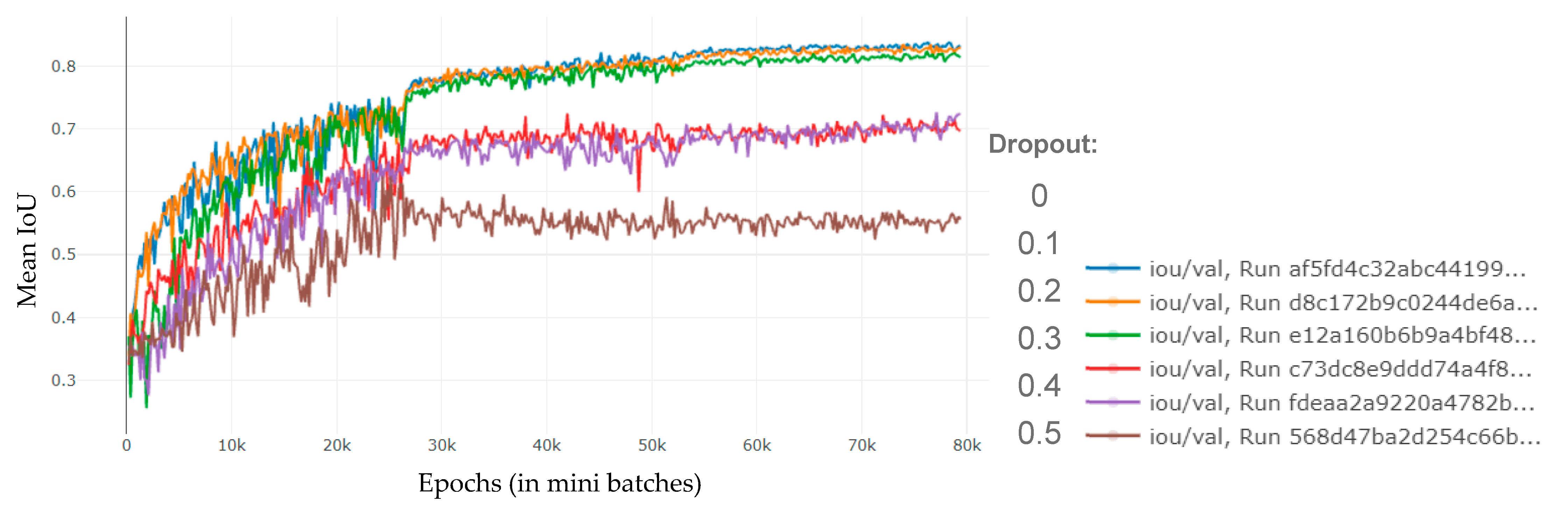
3.4. Dropout as Adaptive Training Regularization

The term “dropped-out” relates to the “filtering-out” of random neurons during the training stage. The process was initially introduced [25] to prevent overfitting by removing unnecessary sets of features for every iteration during the training stage, and it was partially proven to stabilize the prediction while being the regularizer. Table 3 lists the mean IU for respective facies and overall facies, representing sixteen seismic attributes as input and nine seismic attributes as input deployed in A Field, by using different dropout values. Bigger facies classes such as Class IV and Class V (combination of crevasse splays and crevasse channels) show convincing scores that exceed 87 percent. However, it was observed that the network faces difficulty in identifying and predicting small geological features such as Facies Class III (Mud-filled channel). We can conclude that dropout value 0 provides the highest mean IU in the test datasets, while dropout value 0.3 indicates the lowest mean IU in Facies Class IV and V, even using sixteen or nine attributes. These could be possibly due to consistencies in labeling data and accurate augmentation method applied to identify channel and non-channel features. Figure 6 signifies the performance plot using different dropout values during validation phases. Do note that early stopping appears to trigger pre-emptively when setting to monitor validation loss, as validation mean IU visually appears to have further improvement before plateauing possibly due to increased stochasticity in augmentations. Overall, we observed that the application of dropout slows down the learning rate but yields performance improvements on the test dataset when increased gradually from 0 to 0.5.

4. Discussion

4.1. Binary Classification Using Synthetic Model

Figure 7 illustrates small SEAM dataset overlaid by five random north–south and west–east line sections to validate the robustness of the approach. As shown in Figure 8, green arrows indicate structures missed by seismic attributes (inset shown the sweetness attributes). From our observation, even though the size of the trained model is challengingly small (6.4%) compared to the overall SEAM dataset, predicted deepwater channels (Prediction column) matched very well with the labeled data (Ground Truth column), where the validation and test accuracy (in Mean IoU) reached 95% and 85%, respectively. This implies that the 2D U-Net is capable of producing accurate segmented channelized 3D volumes.
We used two scenarios to predict channels in the real dataset:
  • Binary case.
  • Multi-facies case.
In order to produce consistent results, the same algorithms were applied. However, detailed analysis will be discussed in the multi-facies case study, as it deals with the current scenarios in any real data.

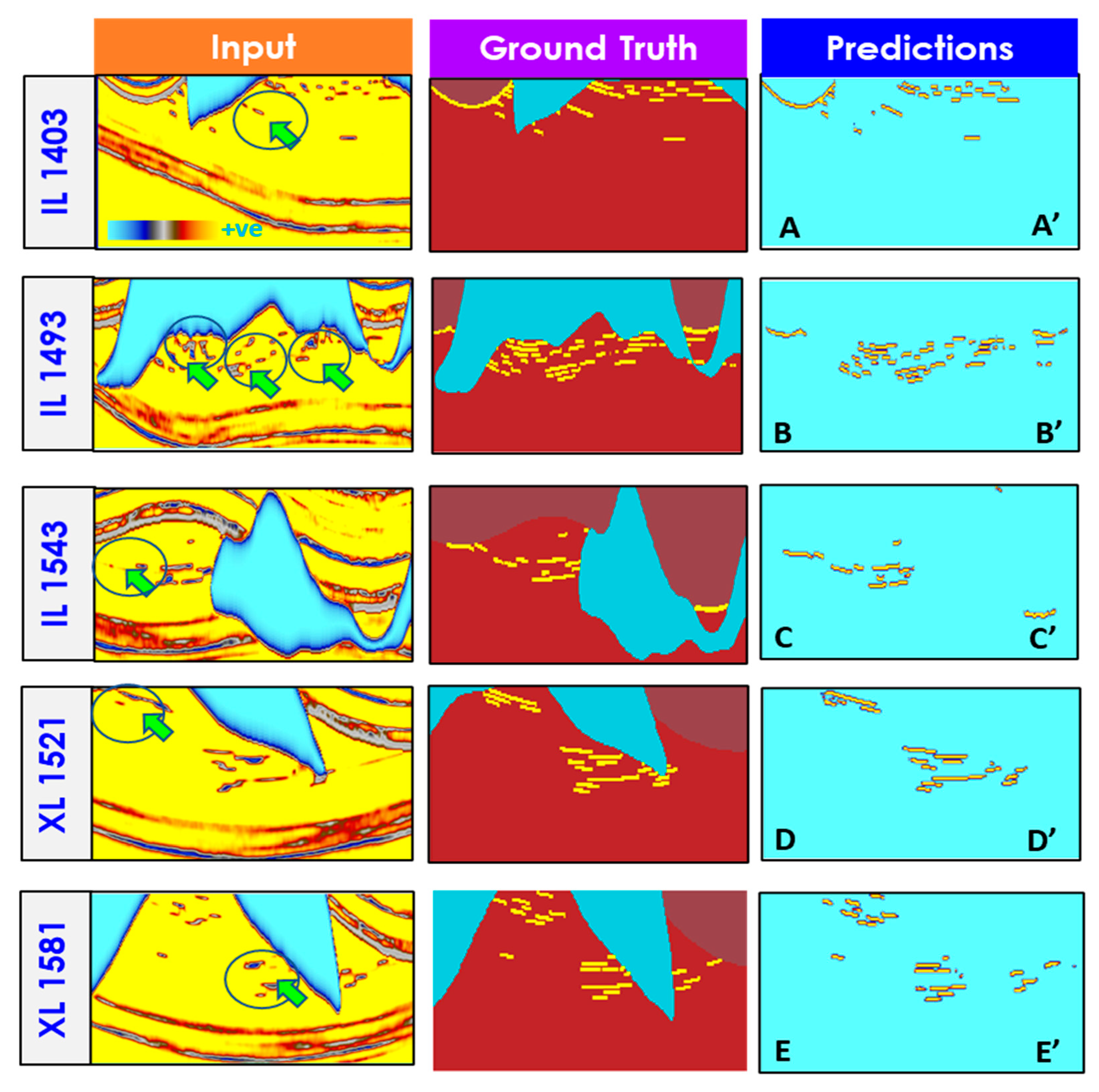
4.2. Channel Detection Using U-Net (Binary Case)

Figure 9a portrays two inline sections representing spectral decomposition volumes after validating the best frequency range to be blended between low, medium, and high volumes, highlighting I-27 to I-35 Lower Reservoir. Log pattern analysis from nearby key wells was observed in both inline 980 and 1070. We display the seismic attribute dataset (inset are shown the sweetness attributes in Figure 9b as part of the input data. Theoretically, sweetness attributes can be generated based on instantaneous amplitude divided by the square root of instantaneous frequency and defined as the trace envelope a(t) divided by the square root of the average frequency fa(t) [26].
In the lens of prospect identification and understanding the reservoir in fluvial settings, sweetness is capable of highlighting hydrocarbon-bearing reservoirs and lithofacies discrimination, given that seismic data quality is conditioned and pre-processed. We chose two different time slices penetrating the studied channelized reservoir interval to identify different fluvial structures, namely, meandering channel, point bars, distributary channels, and mud-filled channels (MFC). Figure 9c depicts the ground truth built using the labeling tool. In order to test the effectiveness for binary classification of fluvial channels, hold-out layers were applied to highlight only on channel and non-channel features during the test stage. It was observed that the network is capable of capturing distributary channels that were missed by sweetness attributes (Figure 9d). Meanwhile, penetrating toward deeper slices shows that MFC are able to be captured by the network even with a small training dataset in Class III.

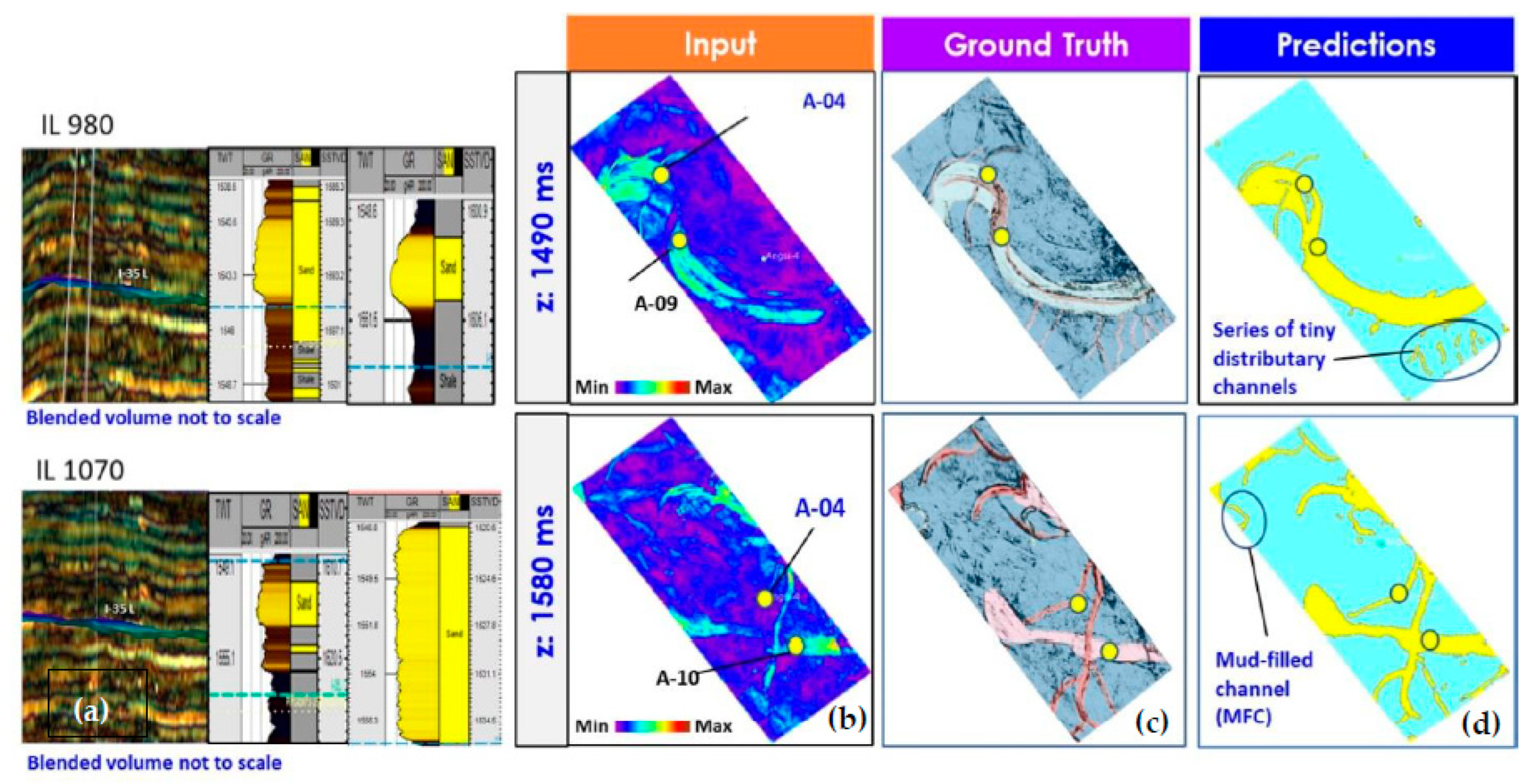
4.3. Channel Detection Using U-Net (Multi-Facies Case)

Figure 10a portrays similar spectral decomposition volumes with log pattern analysis (specifically, from I-27 to I-35 Lower Reservoir) from nearby wells observed in inline 980 and 1070. Figure 10b shows seismic attributes as previously used for binary classification) as part of the input data. Figure 10c depicts the ground truth built using the labeling tool. To test the effectiveness for the second analysis, ten holdout layers were applied for blind-test analysis and five different facies classes were defined in the Python code. It was observed that the neural network is capable of capturing Class I in the shallower section, as shown in Figure 10d. As indicated in the ellipse, MFC still can be detected by the network even when facing a small training dataset in Class III, as observed in the deeper slice.

5. Conclusions

We have discussed an integrated approach of predictive modeling for binary and multi-facies classification using a blob-based and labeling method. We conclude that U-Net is able to classify and automate geobodies with a smaller annotated dataset despite using different ground truth selection. The blob-based method shall minimize the laborious effort needed by the interpreters from manual labeling work. However, it provides flexibility for a field with less well information, low quality of seismic data, and limited interpreted horizons. U-Net remains versatile for different geological complexities without having the need to change the network architecture extensively.
SEAM successfully validated synthetic deepwater channel predictions with mean IoU of 85% using the blob-based method. Further validation was cascaded to a real dataset in binary and multi-facies prediction with high accuracy in multi-facies classes (87 to 90% accuracies) using the labeling tool, with lesser cost and further time saving in prediction and automating geobodies, compared to the conventional method. Key hyperparameters such as dropout slow down the learning rate but yield performance improvements during testing when increased gradually from 0 to 0.5. Selection of smaller learning rate and accurate batch size are also the main keys to improving network accuracy. In the future, imbalance facies distribution or data occlusions in a real field can be reduced by exposing more data representation in vertical or horizontal sections, orthogonal slices, stacked sections, or as a volume, together with a customized time warping approach.

Author Contributions

Conceptualization, S.M.S., N.W.T., M.S., E.A.J.J. and A.H.A.L.; methodology, S.M.S., N.W.T. and M.S.; software, S.M.S., N.W.T. and M.S.; validation, S.M.S. and N.W.T.; formal analysis, S.M.S. and N.W.T.; investigation, S.M.S. and N.W.T.; resources, S.M.S., N.W.T. and M.S.; data curation, S.M.S., N.W.T. and M.S.; writing—original draft preparation, S.M.S.; writing—review and editing, S.M.S., N.W.T. and M.S.; visualization, S.M.S.; supervision, E.A.J.J. and A.H.A.L.; project administration, S.M.S.; funding acquisition, E.A.J.J. All authors have read and agreed to the published version of the manuscript.

Funding

This research was funded by Petroleum Research Fund, PETRONAS.

Institutional Review Board Statement

Not applicable.

Informed Consent Statement

Not applicable.

Data Availability Statement

The data used in this study are confidential and cannot be released.

Acknowledgments

The authors are grateful to PETRONAS for providing the required data and funding for this research work. We would like to thank the ARCC Department, PETRONAS, and all colleagues from the Geoimaging Technology Department for their support and constructive input. We would also wish to thank M. Firdaus, A. Halim, and Junxiao Li as internal reviewers, whose valuable input improved this work.

Conflicts of Interest

The authors declare no conflict of interest.

References

  1. Bridge, J.S. Description and interpretation of fluvial deposits: A critical perspective. Sedimentology 1993, 40, 801–810. [Google Scholar] [CrossRef]
  2. Allen, G.P.; Posamentier, H.W. Transgressive facies and sequence architecture in mixed tide and wave-dominated incised valleys: Example from the Gironde estuary, France. Spec. Publ. 1994, 51, 225–240. [Google Scholar]
  3. Barnes, A. Seismic attributes in your facies. CSEG Rec. 2001, 26, 41–47. [Google Scholar]
  4. Marfurt, K.; Chopra, S. Emerging and future trends in seismic attributes. Lead. Edge 2008, 27, 298–318. [Google Scholar]
  5. Hart, B.S. Channel detection in 3-D seismic data using sweetness. AAPG Bull. 2008, 92, 733–742. [Google Scholar] [CrossRef]
  6. Chopra, S.; Marfurt, K. Seismic Attributes for Prospect Identification and Reservoir Characterization; Society of Exploration Geophysicists: Tulsa, OK, USA, 2007. [Google Scholar]
  7. Roden, R.; Smith, T.; Sacrey, D. Geologic pattern recognition from seismic attributes. Interp 2015, 3, 59–83. [Google Scholar]
  8. Fehler, M.; Keliher, P.J. SEAM Phase I: Challenges of Subsalt Imaging in Tertiary Basins, with Emphasis on Deepwater Gulf of Mexico; Society of Exploration Geophysicists: Tulsa, OK, USA, 2011. [Google Scholar]
  9. Marfurt, K.J.; Chopra, S. Seismic discontinuity attributes and Sobel filtering. CSEG Rec. 2014, 39, 4. [Google Scholar]
  10. LeCun, Y. Learning process in an asymmetric threshold network. In Ecole Superieure D’Lng (Mieurs en Electrotechnique ET Electronique); Springer: Berlin/Heidelberg, Germany, 1985; p. 20. [Google Scholar]
  11. LeCun, Y.; Bengio, Y.; Hinton, G. Deep learning. Nature 2015, 521, 436–444. [Google Scholar] [CrossRef]
  12. Badrinarayanan, V.; Kendall, A.; Cipolla, R. Segnet: A deep convolutional encoder-decoder architecture for image segmentation. IEEE Trans. Pattern. Anal. Mach. Intell. 2017, 39, 2481–2495. [Google Scholar] [CrossRef] [PubMed]
  13. Shi, Y.; Fomel, S.; Wu, X. SaltSeg: Automatic 3D salt segmentation using a deep convolutional neural network. Interpretation 2019, 7, SE113–SE122. [Google Scholar] [CrossRef]
  14. Waldeland, A.; Jensen, A.; Gelius, L.-J.; Solberg, A. Convolutional neural networks for automated seismic interpretation. Lead. Edge 2018, 37, 529–537. [Google Scholar] [CrossRef]
  15. Dunham, M.W.; Welford, K.; Malcolm, A.E. Improved well-log classification using semisupervised label propagation and self- training, with comparisons to popular supervised algorithms. Geophysics 2020, 85, O1–O15. [Google Scholar] [CrossRef]
  16. Dramsch, J.S.; Mikael, L. Deep-learning seismic facies on state-of-the-art CNN architectures. In SEG Technical Program Expanded Abstracts 2018; Society of Exploration Geophysicists: Tulsa, OK, USA, 2018; pp. 2036–2040. [Google Scholar]
  17. Csáji, B.C. Approximation with Artificial Neural Networks. Master’s Thesis, Eotvos Loránd University, Budapest, Hungary, 2001. [Google Scholar]
  18. Di, H.; Alregib, G.; Wang, Z. Why using CNN for seismic interpretation? An investigation. In SEG Technical Program Expanded Abstracts 2018; Society of Exploration Geophysicists: Tulsa, OK, USA, 2018; pp. 2216–2220. [Google Scholar]
  19. Wang, W.; Yang, F.; Ma, J. Automatic salt detection with machine learning. In 80th EAGE Conference and Exhibition Extended Abstracts 2018; European Association of Geoscientists & Engineers: Houten, The Netherlands, 2018; pp. 1–5. [Google Scholar]
  20. Pham, N.; Fomel, S.; Dunlap, D. Automatic channel detection using deep learning. Interpretation 2019, 7, 43–50. [Google Scholar] [CrossRef]
  21. Wu, X.; Guo, Z. Detecting faults and channels while enhancing seismic structural and stratigraphic features. Interpretation 2019, 7, T155–T166. [Google Scholar] [CrossRef]
  22. Malik, F. Understanding Neural Network Neurons. 2019. Available online: Medium.com (accessed on 14 August 2022).
  23. Schelhamer, E.; Long, J.; Darrell, T. Fully convolutional networks for semantic segmentation. IEEE Trans. Pattern. Anal. Mach. Intell. 2017, 39, 640–651. [Google Scholar] [CrossRef] [PubMed]
  24. Ronneberger, O.; Fischer, P.; Brox, T. U-Net:Convolutional networks for biomedical image segmentation. In International Conference on Medical Image Computing and Computer-Assisted Intervention; Springer: Berlin/Heidelberg, Germany, 2015; pp. 234–241. [Google Scholar]
  25. Hinton, G.E.; Srivastava, N.; Krizhevsky, A.; Sutskever, I.; Salakhutdinov, R. Improving neural networks by preventing co-adaptation of feature detectors. arXiv 2012, arXiv:1207.0580, arXiv:1207.0580. [Google Scholar]
  26. Radovich, B.J.; Oliveros, R.B. 3-D sequence interpretation of seismic instantaneous attributes from the Gorgon field. Lead. Edge 1998, 17, 1286–1293. [Google Scholar] [CrossRef]
Figure 1. The stratigraphy of the SEAM dataset. (a) The overall SEAM Reservoir Model shows three major reservoirs: sheet turbidites, localized turbidite fans, and channel complexes. The red rectangle shows the area of study selected for channelized predictions. (b) Examples of intersecting channel complexes colored by volume of shale (vshale), with estimated distance 33 km. Modified after [8]. (c) Volume of shale at east–west section at Y = 20 k, showing the interval of interest highlighted by the red rectangle.
Applsci 12 09032 g001
Figure 2. Schematic map of main reservoirs in A Field.
Applsci 12 09032 g002
Figure 3. Integrated methodology applied in this study consists of four main steps: 1. Exploratory Data Analysis (EDA) for input data; 2. Define the ground truth based on two scenarios; 3. Train the dataset and monitor the model’s performance; 4. Geobody extraction to be integrated with another relevant dataset.
Applsci 12 09032 g003
Figure 4. Sixteen types of seismic attributes extracted from A Field. Three different frequency volumes were blended to generate Spectral Decomposition volumes in the I-35 Lower Reservoir.
Applsci 12 09032 g004
Figure 5. Detailed description of fluvial facies elements, as observed in time slice 1564 milliseconds.
Applsci 12 09032 g005
Figure 6. Performance plot represents different dropout values ranging from 0 to 0.5 during validation stages. All experiments show a similar progress pattern before reaching plateau phase due to the stochasticity of data augmentations.
Applsci 12 09032 g006
Figure 7. Overview of training dataset from SEAM Phase I illustrating five (5) cross-sections (A–A’), (B–B’), (C–C’), (D–D’) and (E–E’) cutting across SEAM Reservoir Model. Blue lines represent inline sections, and the remaining lines represents the crosslines.
Applsci 12 09032 g007
Figure 8. Overall input dataset, label data and prediction results from the five (5) geological cross-sections. (Input Column): Green arrows indicate subtle distributary channel series unable to be captured by sweetness attributes. (Ground truth Column): The dataset was built using a blob-based method where facies have been re-classified into binary dataset. (Prediction Column): Good quality of ground truth dataset is capable of guiding the neural network in achieving higher prediction accuracy.
Applsci 12 09032 g008
Figure 9. The results for binary facies classification in A Field. (a) Two random sections of blended spectral decomposition cubes passing through three key wells showing log pattern analysis in the channelized reservoir interval. Two different time slices in (b) portray comparisons between multi-attributes as the input (inset are the sweetness attributes). (c) The labeled data prepared by a human interpreter. Results from binary classification (d) show that the trained neural network is still capable of capturing Class III facies and distributary channels, as indicated in the ellipse, despite dealing with the challenge of imbalanced facies.
Applsci 12 09032 g009
Figure 10. The results for multi- facies classification in A Field. (a) Two random sections of blended spectral decomposition cubes passing through three key wells showing log pattern analysis in the channelized reservoir interval. Two different time slices in (b) display comparisons between multi-attributes as the input (sweetness attributes shown as the example). (c) The labeled data prepared by a human interpreter. Results from multi-facies classification (d) show that the trained neural network is capable of capturing Class III facies, as indicated in the ellipse, despite dealing with the challenge of facies imbalance.
Applsci 12 09032 g010
Table 1. Seismic attribute classification used as guided by [7].
CategoryClassType
Instantaneous
Attributes
IReflection Strength, Instantaneous Phase, Instantaneous
Frequency, Quadrature, Instantaneous Q
Lithology Contrasts, Bedding Continuity, Porosity, DHIs, Stratigraphy, Thickness
Geometric
Attributes
IISemblance and Eigen-Based Coherency/Similarity, Curvature (Maximum, Minimum, Most Positive, Most Negative, Strike, Dip)Faults, Fractures, Folds
Anisotropy, Regional Stress Fields
Amplitude-Accentuating
Attributes
IIIRMS Amplitude, Relative Acoustic Impedance, Sweetness, Average EnergyPorosity, Stratigraphic and Lithologic
Variations, DHIs
AVO AttributesIVIntercept, Gradient, Intercept/Gradient Derivatives
Fluid Factor, Lambda–Mu-Rho, Far–Near, (Far–Near) Far
Pore Fluid, Lithology, DHIs
Seismic Inversion
Attributes
VColored Inversion, Sparse Spike, Elastic Impedance
Extended Elastic Impedance, Prestack Simultaneous
Inversion, Stochastic Inversion
Lithology, Porosity, Fluid
Effects
Spectral
Decomposition
VIContinuous Wavelet Transform, Matching Pursuit
Exponential Pursuit
Layer Thicknesses, Stratigraphic Variations
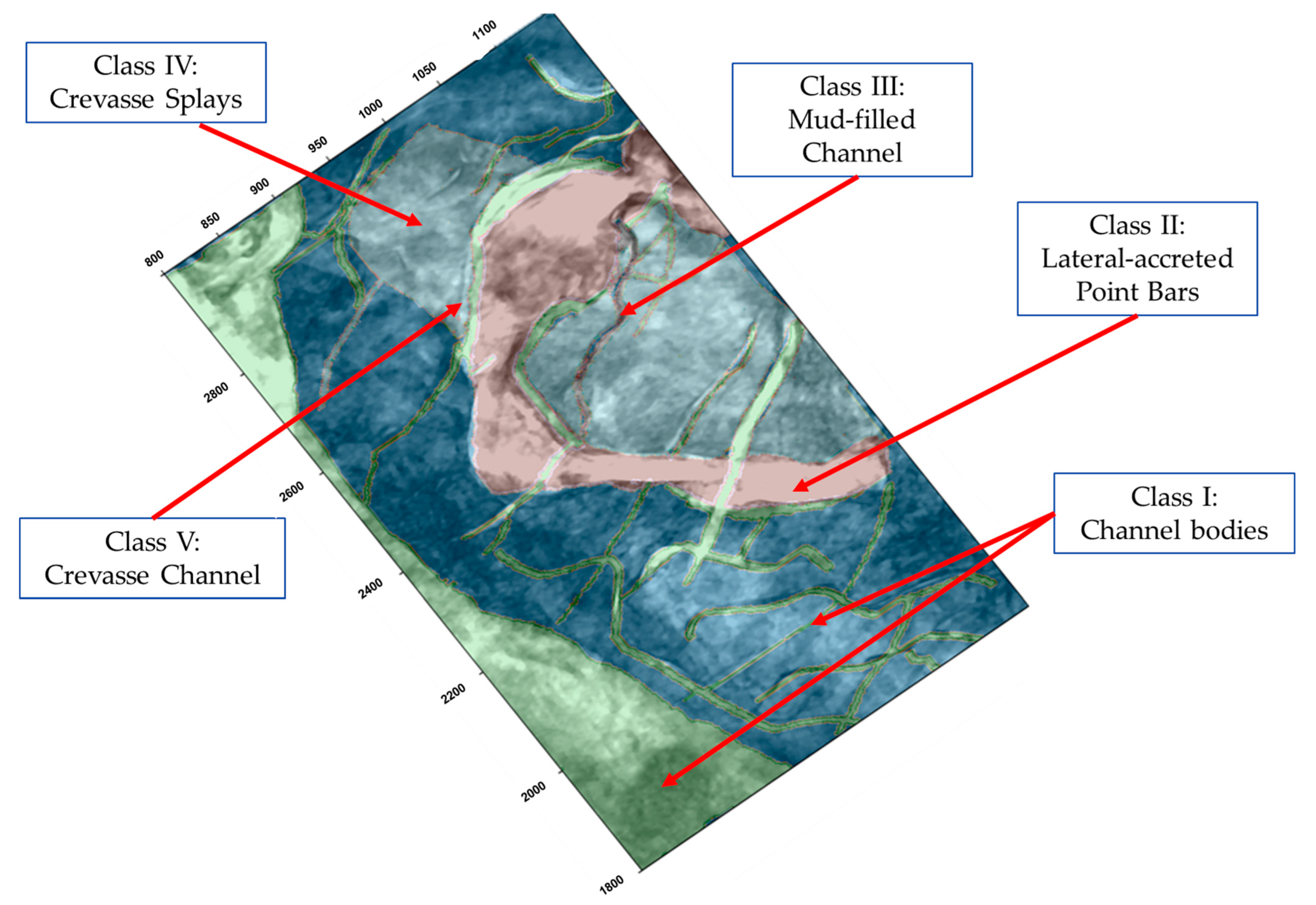
Table 2. The percentage of pixels for each facies class in the training dataset of A Field.
Class I
(Channel)
Class II
(Point Bar)
Class III
(Mud-Filled Channel)
Class IV and V
(Crevasse Splays and Crevasse Channel)
7.124.150.1688.57
Table 3. Results in the two categories, with dropout variations, in the test dataset. All metrics are in the range of 0 to 1, with larger values being better. The best-performing model for every metric is highlighted in bold.
InputAttributesDropoutFacies Accuracy:Overall Mean IoU
Class IClass IIClass IIIClass IV and V
16 Features0.00.6710.7620.3440.9040.670
0.10.6880.6520.2540.9070.650
0.20.6520.7850.3280.9050.667
0.30.6400.6820.3100.8930.631
9 Features0.00.6810.7660.3220.9050.668
0.10.7020.7570.3020.9070.651
0.20.6150.7000.2560.8720.611
0.30.6660.6680.2930.8820.631
Publisher’s Note: MDPI stays neutral with regard to jurisdictional claims in published maps and institutional affiliations.

