Fault Detection of Landing Gear Retraction/Extension Hydraulic System Based on Bond Graph-Linear Fractional Transformation Technique and Interval Analytic Redundancy Relations

Featured Application

In the research on fault detection of landing gear retraction/extension hydraulic system, bond graph linear fractional transformation technology and interval analysis theory are applied to consider uncertain negative factors in the system, improving the accuracy and sensitivity of fault detection.

Abstract

Fault detection in the landing gear retraction/extension hydraulic system is difficult due to uncertainties in component parameters and sensor measurement values. This work lies in the introduction of linear fractional transformation technology and uncertainty analysis theory for the construction of the diagnostic bond graph of the landing gear retraction/extension hydraulic system. Thus, interval analytical redundancy relations can be derived as well as fault signature matrices. By using the fault signature matrix, existing faults can be detected and isolated preliminary. Furthermore, interval analytical redundancy relations can be used to detect system faults in detail. The analysis results of the failure cases of the internal and external leakage of the actuator and landing gear selector valve reversing stuck show that compared to the traditional analytical redundancy relations, this method takes into account the negative factors of uncertainty, so it can effectively reduce missed diagnosis and misdiagnosis; compared to the traditional absolute diagnostic threshold, the interval diagnostic threshold is more accurate and sensitive.

1. Introduction

According to Boeing, Airbus, EASA (European Union Aviation Safety Agency), and ICAO (International Civil Aviation Organization) [1,2,3,4], more than 50% of fatal accidents occur during final approach and landing. Due to its irreplaceable nature, landing gear performance directly affects aircraft takeoffs and landings. A significant part of the landing gear retraction/extension process is the retraction/extension (R/E) hydraulic system. Hydraulic transmissions, in comparison with gear mechanical transmissions, are able to achieve a wide range of stepless speed regulation, which is essential to the smooth retraction/extension of landing gears within the specified timeframe [5,6]. Fault detection, on the other hand, is the first step in implementing fault diagnosis technology. Unless the detection is accurate and effective, it will be difficult to isolate faults in the future, and it will also affect subsequent health assessment and maintenance. It is therefore essential to detect faults accurately.

Research methods for fault diagnosis of complex nonlinear systems such as hydraulic systems fall into three categories: knowledge-based, data-driven, and model-based [7]. In knowledge-based methods, knowledge reasoning and long-term accumulated experience knowledge are mainly used [8,9,10]. In data-driven analysis, a large amount of online and offline data from the system is analyzed [11,12,13,14]. Sara Nasiri and others [15] have made a detailed review of fault failure analysis in the traditional mechanical field from the perspective of artificial intelligence, involving artificial neural networks, Bayesian networks, genetic algorithms, fuzzy logic, and case-based reasoning.

Based on a model-based approach, this work examines whether there is a consistency criterion between the system’s actual output and its expected output. State estimation methods, parameter estimation methods, and equivalent space methods are kinds of model-based methods.

Generally, state estimation methods compare the state output of the system model with the output of the actual system to generate system residuals that are used as consistency criteria. Observer and filter methods are used, with Kalman filter being the most commonly used. Most of the studied systems are nonlinear systems, which are inevitably affected by various factors such as the uncertainty of model parameters, the interaction between components and systems, the interaction between environment and systems, and noise. Therefore, most experts and scholars mainly focus on the robust state estimation of nonlinear systems. In the research of observer methods, Hu Zhenggao [16] proposed nonlinear adaptive unknown input observer, Liu Yingming [17] studied the sliding mode control of rolling mills using a disturbance observer, and Xu Guosheng [18] studied the sliding mode control of excavator based on a high-gain observer. In the research of the Kalman filter, various improved Kalman filters or their variants have been produced, such as the extended Kalman filter [19], multiple outlier robust Kalman filter [20], federated Kalman filter [21], unscented Kalman filter [22], distributed Kalman filter [23], etc.

In the parameter estimation method, the estimated physical parameters are compared with the nominal values in order to generate the system residual. This serves as a consistency criterion for the core idea. There are two common estimation methods: joint estimation and minimum error estimation. In the joint estimation method [24,25], the estimated parameters are used as the extension of the state, and the state estimation method is used to estimate the state and parameter. Despite its simplicity and speed, this method may result in dimension disaster if the space dimension is too high after expansion. Compared to the extended state space method, the method based on multi structure observer and filter [26] has stronger robustness and lower computational difficulty. Further, the minimum error method [27] is mostly used for off-line fault diagnosis, and its accuracy depends on the completeness of data samples.

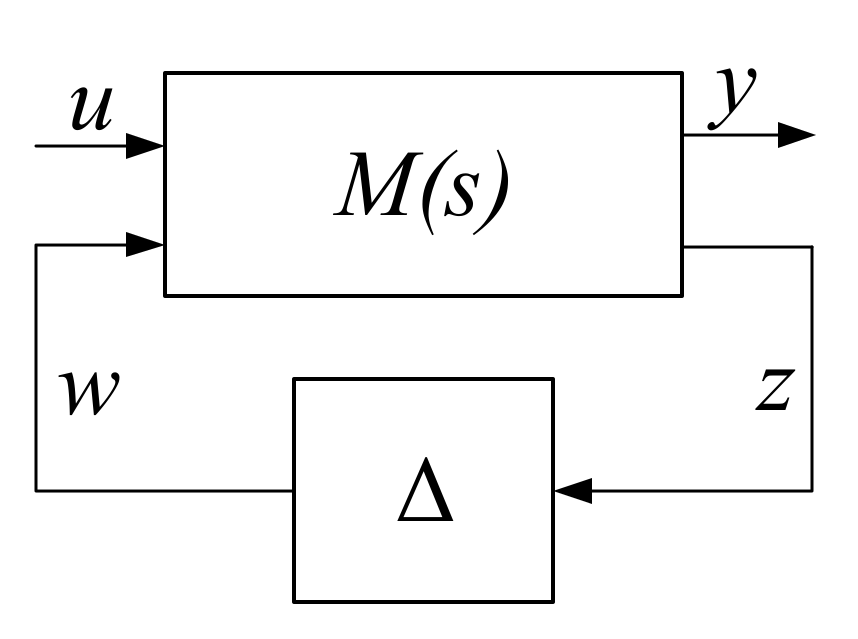
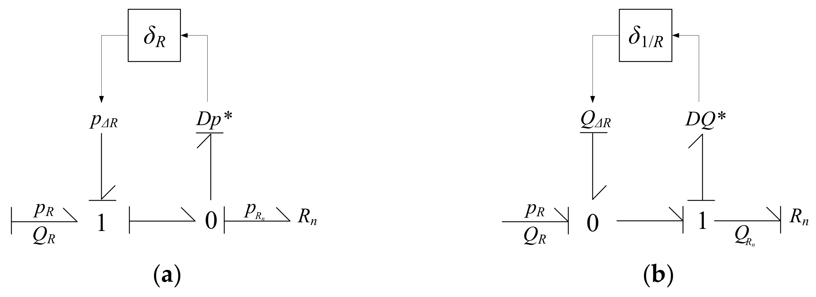
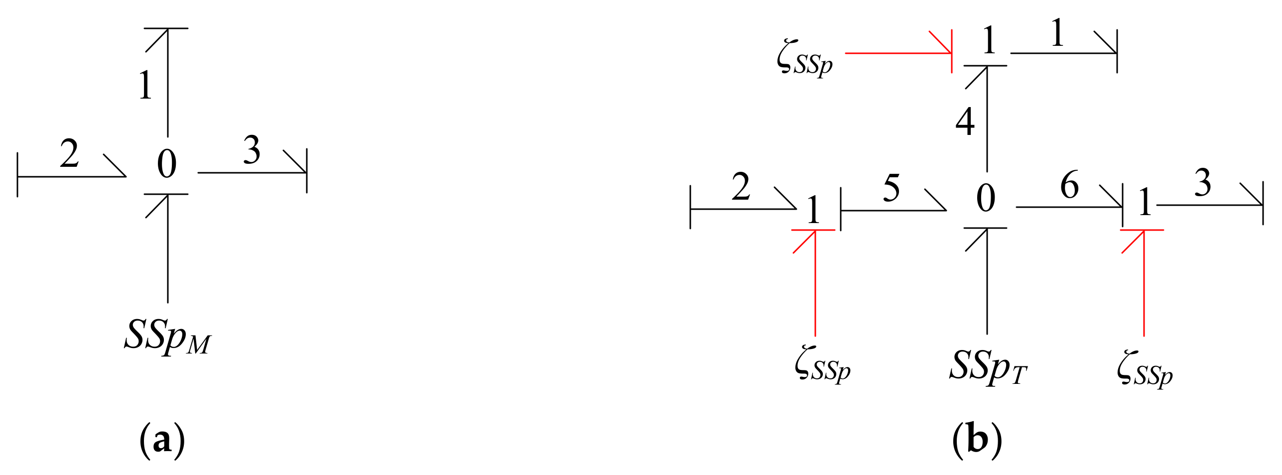
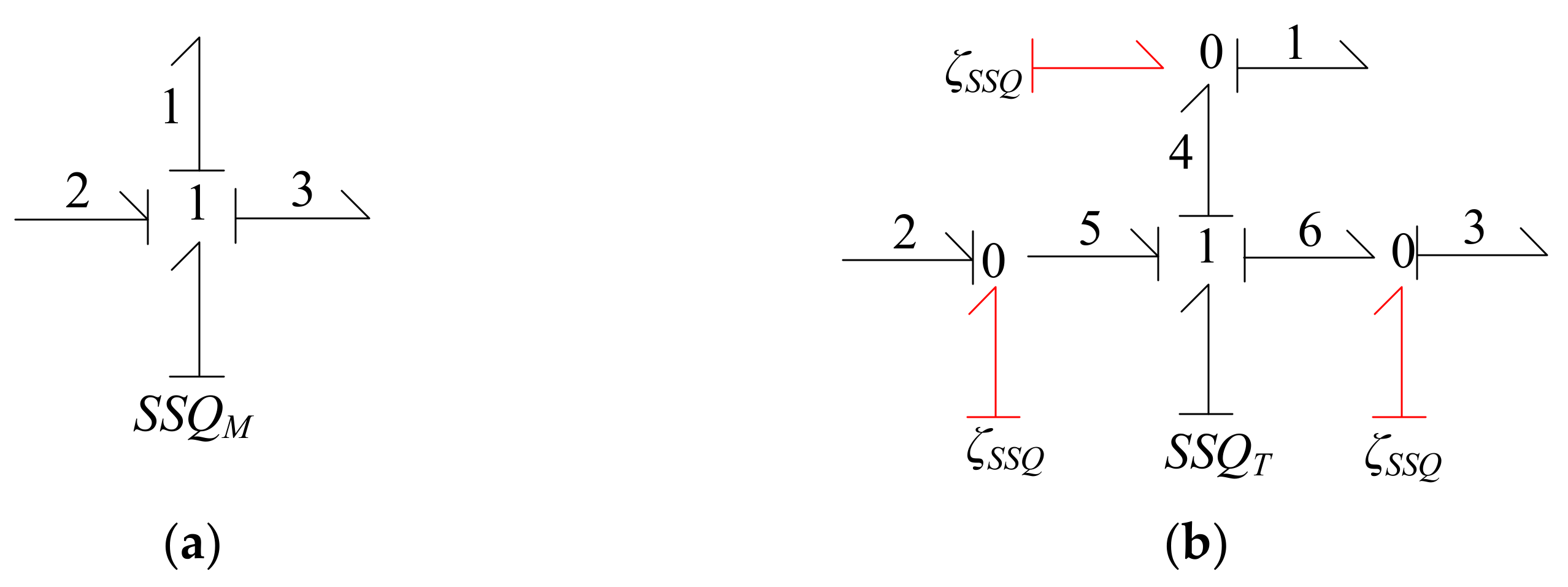
A core principle of equivalent space method is to use the residual between the input and output of the analytical model of the system as a consistency criterion. Using hardware redundancy, multiple redundant sensors are set up and residuals are derived from the measurement model for analysis. Although this method is simple and easy, it also requires multiple redundant sensors, so its cost is high. As a consistency criterion of the core diagnosis idea, an analytical redundancy relations (ARRs) method builds the residual indirectly through an analytical mathematical model. Using a power bond graph and relying on the energy conservation law, this method has some drawbacks, including parameter uncertainty, sensor measurement uncertainty, environmental impact, and noise. As a result, the residual generated by the system will fluctuate, leading to misdiagnosis and missed diagnoses. It is necessary to incorporate system uncertainty robustness into the bond graph model to improve this problem. Bond graph-linear fractional transformation (BG-LFT) is the most effective solution to this problem. On the basis of this technology, Mo Haobin [28] proposed a fault diagnosis method based on interval analytical redundancy relationships in order to avoid the interference of system uncertainty on diagnosis results. Wang Fang [29] designed a robust diagnosis observer for hybrid systems, and combined BG-LFT and proportional integrator to realize robust fault diagnosis and estimation, which improved the detection effect. M.A. Djeziri [30] believes that all uncertainties are cumulative in the diagnosis threshold of node residual. In this way, uncertainty interaction will be ignored, which may lead to overestimation of the diagnosis threshold.

The previous literature [31] mainly focuses on evaluating the system’s health after fault detection. This paper is an application-oriented innovation that focuses on detecting faults accurately, so that the process of fault detection can be improved. On the basis of the uncertain interference factors, this paper addresses the goal of accurately detecting the preset faults of the landing gear R/E hydraulic system. 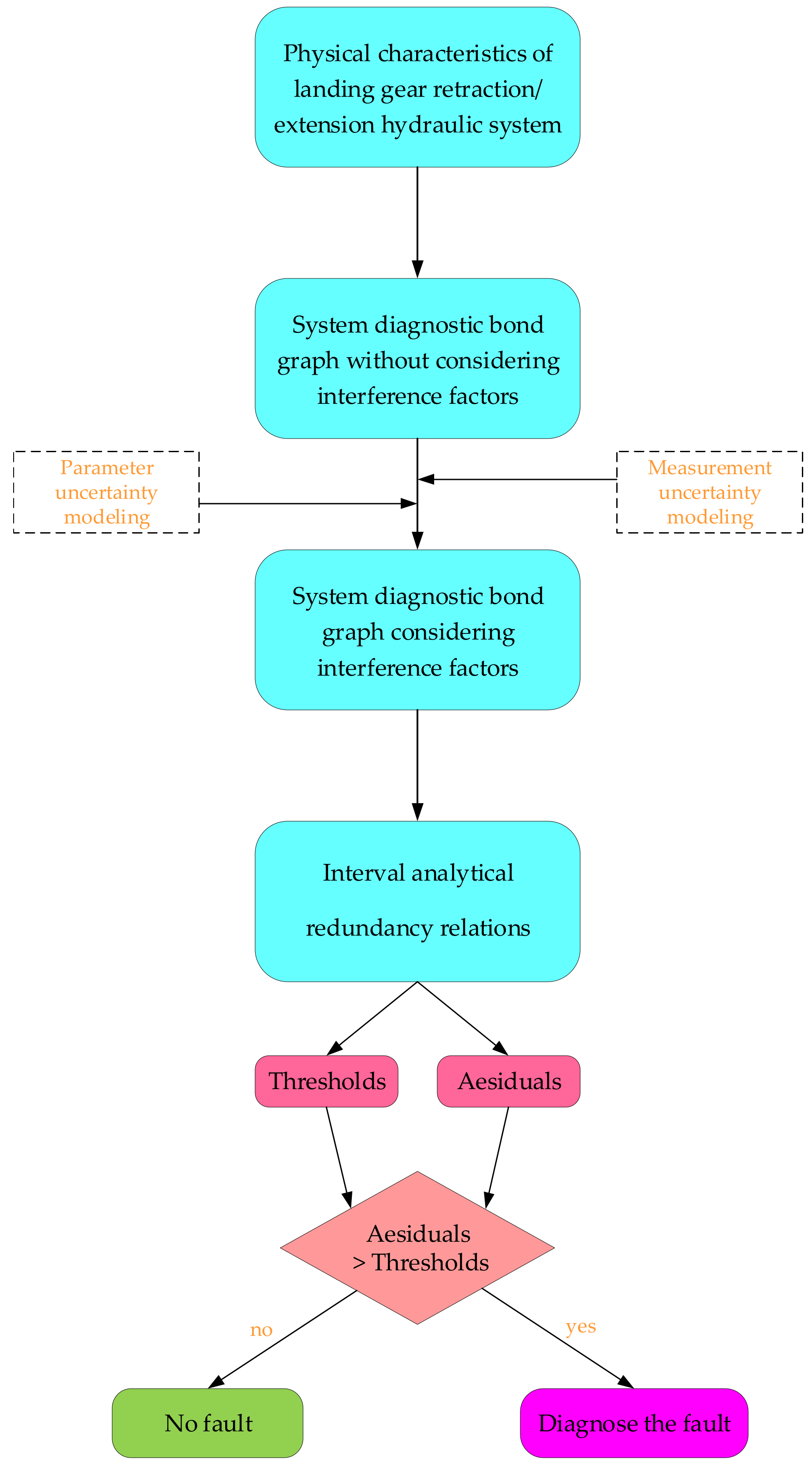Figure 1 illustrates the analysis process and train of thought. Contributions include:

• When studying fault diagnosis for dynamic system models, various uncertain interference factors must be taken into account. For this reason, bond graph linear fractional transformation and interval analytical redundancy relations are used together.
• Preliminarily, the relevant landing gear R/E hydraulic fault parameters are detected and isolated using the fault signature matrix (FSM).
• Asymmetric interval thresholds have better detection accuracy and sensitivity than absolute thresholds, according to fault case analyses.

Figure 1. Analysis process and train of thought.

Figure 1. Analysis process and train of thought.

2. Overview of Landing Gear Retraction/Extension Hydraulic System and Its Traditional Diagnosis Bond Graph

2.1. Basic System Framework

According to the literature [32,33], the basic framework of the landing gear retraction/extension (R/E) hydraulic system can be constructed, as shown in Figure 2. It is basically the same system architecture diagram as the previously published article [31], but with slight differences. Hydraulic power is provided by both electric motor-driven pumps and engine-driven pumps, along with other accessories. A landing gear selector valve distributes hydraulic oil to the hydraulic components of left and right MLG (main landing gear) and NLG (nose landing gear). Check valves, throttle valves, and hydraulic fuses are not shown in Figure 2, which only shows the most important parts of the function.

In the subsequent bond graph modeling, the generalized potential variable $e$ in the hydraulic system refers to the pressure $p$ and the generalized flow variable $f$ refers to the flow rate $Q$ [34]. All models must satisfy the fundamental requirements of equal pressure at the common potential node (0-node) and equal flow at the common flow node (1-node). On the half-tip arrow’s side are state and variation quantities of pressure, whereas on the side without the tip are state and variation quantities of flow. An entire arrow indicates a signal bond between the parameters at its two ends, which indicates a functional relationship.

2.2. Modeling of Landing Gear Selector Valve

Figure 3a illustrates the physical essence of the landing gear selector valve, which is a Y-type, three-position, four-way solenoid directional valve. When the P-port is closed and the A, B, and T ports are connected, the floating piston, the ability to move in response to external forces, and hydraulic pump not unloading are the characteristics that define its median function. Figure 3b–d depict the landing gear selector valve’s neutral, left, and right operational states. Figure 4 depicts the bond graph model of the landing gear selector valve.

Port P is the supply port, Port T is the return port, and Ports A and B are connected to the subsequent pipes. Four paths (PA, PB, AT, BT) are formed by the valve body and spool’s relative positions, and the corresponding fluid resistance are $R_{PA}$, $R_{PB}$, $R_{AT}$, and $R_{BT}$.

Neutral, left, and right working states have the following meanings [35]:

(1)

Neutral: Now that the high-pressure source P port is disconnected from the system, the A and B ports are attached to the return port T. Hydraulic oil returns to the tank through the hydraulic resistance $R_{AT}$ of the AT path and the hydraulic resistance $R_{BT}$ of the BT path, respectively. At this time, liquid resistance $R_{PA}$ and $R_{PB}$ are not considered.

(2)

Left: Port A is connected to the return port T, whereas port B is connected to the high-pressure source port P. Through $R_{PB}$ of the PB path, the high-pressure hydraulic oil exits from port B. Through $R_{AT}$ of the path AT, hydraulic oil from the return line flows back to the tank. Liquid resistance $R_{PA}$ and $R_{BT}$ are not taken into consideration at this time.

(3)

Right: Port B is connected to the return port T, whereas port A is connected to the high-pressure source port P. Through $R_{PA}$ of the PA path, high-pressure hydraulic oil exits from port A. Through $R_{BT}$ of the path BT, hydraulic oil from the return line flows back to the tank. Liquid resistance $R_{PB}$ and $R_{AT}$ are not taken into consideration at this time.

2.3. Modeling of Actuator

Actuators convert hydraulic energy into mechanical energy in order to reciprocate linear motion in hydraulic systems. Landing gear R/E hydraulics include the main landing gear actuator, downlock actuator, uplock actuator, nose landing gear actuator, and lock actuator [36]. The transfer cylinder can be regarded as an actuator with a diameter of 0 on both sides of the piston rod. Since all actuators have the exact same physical characteristics, only one modeling is needed. Although there are many actuators in the system, by only using the R/E actuator as terminals, the analysis is made simpler. Figure 5 illustrates the model, and

Table 1. Parameters definition of actuators bond graph.

Parameter Name	Meaning
$p_{Rodless}$$Q_{Rodless}$	Pressure and flow of rodless cavity
$p_{Rod}$$Q_{Rod}$	Pressure and flow of rod cavity
$A_{Rodless}$$F_{Rodless}$	Acting area and force of piston on one side of rodless cavity
$A_{Rod}$$F_{Rod}$	Acting area and force of piston on one side with rod cavity
$v$	Piston velocity
$R_{Ex-l}$	Hydraulic resistance effect of external leakage of actuator
$C_{Ex-Rodless}$$C_{Ex-Rod}$	Liquid capacity effect of rodless cavity and rodless cavity
$R_{In-l}$	Hydraulic resistance effect of internal leakage of actuator
$R_{Eq-f}$	Equivalent friction liquid resistance effect of reciprocating motion outside the actuator
$F_{ex}(x)$	Other external forces acting on external loads

defines the actuator parameters.

2.4. Modeling Rules and Diagnostic Bond Graph

Figure 6 illustrates the traditional diagnostic bond graph of the system. According to the literature [37], the following guidelines were used to determine the causal relationship:

• There is a sole causal relationship between the potential source and the flow source, with the potential source’s causality stroke on the side closest to the tip and the flow source’s causality stroke on the side furthest from the tip.
• Both inertial and capacitive elements have precedence for defining integral causality, but the causality of the inertial element is on the side closest to the tip, whereas the causality of the capacitive element is on the side farthest from the tip.
• The resistive component prioritizes admittance-type causality; the causality stroke is on the tip side, but coordination with other bond graph parts must be taken into account throughout the designation process, and the causality is extended in the direction of flow at the node.

Each bond and node are numbered according to the following principles:

• Starting from number 1, each bond is numbered in turn, counterclockwise, centered on the node, and the signal bonds are not numbered.
• Starting from number (1), each node is numbered according to the direction of energy flow, and the converter $TF$ node is not numbered.

Figure 6. Traditional diagnostic bond graph of landing gear R/E hydraulic system.

Figure 6. Traditional diagnostic bond graph of landing gear R/E hydraulic system.

In Figure 6, the pre-defined fault nodes and the nodes where multiple bonds converge in the system are chosen as the virtual sensor placement locations. To detect the pressure signal, the pressure sensor SSp is placed at the common potential node (0-node), and to detect the flow signal, the flow sensor SSQ is placed at the common flow node (1-node).

Table 2. Set virtual sensors and corresponding ARRs.

Pressure Virtual Sensor	Flow Virtual Sensor
$SS{p}_1 \mathrm{and} SS{p}_3:{\mathrm{ARR}}_1$	$SS{Q}_1:{\mathrm{ARR}}_3$
$SS{p}_2 \mathrm{and} SS{p}_4:{\mathrm{ARR}}_2$	$SS{Q}_2:{\mathrm{ARR}}_4$

displays the correspondence between the sensor and analytical redundancy relations (ARRs).

Due to the simplified construction model in this paper, there are only four residuals generated, of which two sensors generate one ARR. When the model is complex and delicate, dozens or even hundreds of residuals will be generated, and each residual will show a very different detection effect. There are not many residuals with good detection effects. Based on convex optimization, Daniel Jung and others [38] investigated selecting residuals with better detection performance from a large number of residuals.

3. Modeling Method Considering Uncertainty

3.1. Uncertainty Modeling of Component Parameters

Bond graph-linear fractional transformation technique (BG-LFT) [39] is a widely used and effective method for research considering system uncertainty. Figure 7 is a general model of the method.

In Figure 7, $M(s)$ is an incidence matrix; $\Delta$ is the parameter uncertainty deviation matrix; $u$ and $y$ are actual input and output vectors, respectively; $w$ and $z$ are auxiliary input and output vectors, respectively.

Under the premise of not changing the causality of the original bond graph model, the uncertainty is expanded. Let the true values of the resistive element $R$, capacitive element $C$ and inertial element $I$ of the bond graph model be $\theta \in \{R,C,I\}$, the nominal value be ${\theta }_n\in \{R_n,C_n,I_n\}$ and the uncertainty value be $\theta \in \{\Delta R,\Delta C,\Delta I\}$.Then each value satisfies:

$$\theta ={\theta }_n+\Delta \theta$$

(1)

Define $\delta =\Delta \theta /\theta$ as relative uncertainty. Taking the resistive element as an example, it can be specifically expressed as follows:

$$\left\{\begin{array}{l}\mathrm{Impedance} \mathrm{type}:p_R=Q_{R}R=Q_R(R_{\theta }+\Delta R)=Q_R{R}_{\theta }(1+{\delta }_R)=p_{R_n}+p_{\Delta R}\\ \mathrm{Admittance} \mathrm{type}:Q_R=\frac{p_R}{R}=\frac{p_R}{R_{\theta }+\Delta R}=\frac{p_R}{R_n}(1-\frac{\Delta R}{R_n+\Delta R})=Q_{R_n}+Q_{\Delta R}\end{array}\right.$$

(2)

where $p_R$ is the actual output pressure, $Q_R$ is the actual input flow, $p_{R_n}$ is the nominal pressure of the element, and $p_{\Delta R}$ is the uncertainty pressure. The resulting image is shown in Figure 8.

BG-LFT models of capacitive elements and inertial elements can be obtained by the same method, as shown in Figure 9 and Figure 10 where $Dp*$ and $DQ*$ are sensor virtual pressure source and flow source, respectively.

3.2. Uncertainty Modeling of Sensor Measurement

Due to negative factors such as environmental impact and noise, the measured value of the sensor is often not the true value, and there is an inevitable error [40,41]. Let the true value of the sensor be $S_T\in \{SS{p}_T,SS{Q}_T\}$, the measured value be $S_M\in \{SS{p}_M,SS{Q}_M\}$, and the measurement error be $\Delta S\in \{{\zeta }_{SSp},{\zeta }_{SSQ}\}$. They have the following relationships:

$$S_T=S_M+\Delta S$$

(3)

Specific modeling of 0-node a is as follows:

Figure 11a is a model without consideration of measurement uncertainty, and Figure 11b is a model with consideration of measurement uncertainty.

Therefore, considering the uncertainty of the measured value of the sensor, its true value is:

$$\left\{\begin{array}{l}{p}_1=p_2=p_3=SS{p}_M\\ p_1=p_4+{\xi }_{SSp}=SS{p}_M+{\xi }_{SSp}\\ p_2=p_5+{\xi }_{SSp}=SS{p}_M+{\xi }_{SSp}\\ p_3=p_6+{\xi }_{SSp}=SS{p}_M+{\xi }_{SSp}\end{array}\right.$$

(4)

Specific modeling of 1-node a is as follows:

Figure 12a is a model without consideration of measurement uncertainty, and Figure 12b is a model with consideration of measurement uncertainty.

Therefore, considering the uncertainty of the measured value of the sensor, its true value is:

$$\left\{\begin{array}{l}{Q}_1=Q_2=Q_3=SS{Q}_M\\ Q_1=Q_4+{\xi }_{SSQ}=SS{Q}_M+{\xi }_{SSQ}\\ Q_2=Q_5+{\xi }_{SSQ}=SS{Q}_M+{\xi }_{SSQ}\\ Q_3=Q_6+{\xi }_{SSQ}=SS{Q}_M+{\xi }_{SSQ}\end{array}\right.$$

(5)

3.3. Model Extension Based on Interval Analytic Redundancy

Taking the resistive element as an example, for any pressure variable $p$:

$$p=(R_n+\Delta R)(SS{Q}_M+{\zeta }_{SSQ})=R_{n}SS{Q}_M+[(R_n+\Delta R){\zeta }_{SSQ}+\Delta R\cdot SS{Q}_M]$$

(6)

Therefore, $p_u=[(R_n+\Delta R){\zeta }_{SSQ}+\Delta R\cdot SS{Q}_M]$ is defined as an uncertainty term and $R_{n}SS{Q}_M$ is the residual term without considering the uncertainty.

Traditional analytical redundancy relations (ARRs) [42] are a constraint relationship obtained from a system model based on energy conservation rules.

$$\left\{\begin{array}{l}{\mathrm{ARR}}_i=f_i(k_i,{\theta }_i) i=1,\cdots ,n\\ \mathrm{ARRs}=[{\mathrm{ARR}}_1,{\mathrm{ARR}}_2,\cdots ,{\mathrm{ARR}}_n]\\ r_i={\mathrm{ARR}}_i=0\end{array}\right.$$

(7)

where $i$ is the number of the ARR, $k_i$ is the system variable, ${\theta }_i$ is the system parameter, and $f_i$ is a function of the $k_i$ and ${\theta }_i$. $r_i$ is the residual generated by the system node.

After introducing the theory of interval analytic redundancy, the traditional analytic redundancy is extended. $\left[{\delta }_{\theta }\right]=\left[-\Delta {\theta }_l/{\theta }_n,\Delta {\theta }_r/{\theta }_n\right]$ is defined as the relative uncertainty of parameter interval. For parameter uncertainty:

$$\left[\underset{¯}{\theta },\overline{\theta }\right]=\left[{\theta }_n-\Delta {\theta }_l,{\theta }_n+\Delta {\theta }_r\right]={\theta }_n(1+\left[{\delta }_{\theta }\right])$$

(8)

where $\overline{\theta }$ and $\underset{¯}{\theta }$ are the upper and lower limits of parameters, respectively. $-\Delta \theta$ and $\Delta {\theta }_r$ are the left and right extreme values of parameter uncertainty respectively.

For measurement uncertainty:

$$\left[\underset{¯}{S_T},\overline{S_T}\right]=\left[S_M-\Delta S_l,S_M+\Delta S_r\right]=S_M+\left[{\xi }_S\right]$$

(9)

where $\overline{S_T}$ and $\underset{¯}{S_T}$ are the upper and lower limits of true value. Respectively. $-\Delta S_l$ and $\Delta S_r$ are the left and right extreme values of measurement uncertainty, respectively.

Therefore, for pressure variable $p$, the expanded system level interval analytical redundancy relations are:

$$p=\left[\underset{¯}{R},\overline{R}\right]\cdot \left[\underset{¯}{SS{Q}_T},\overline{SS{Q}_T}\right]=R_{n}SS{Q}_M+(R_{n}SS{Q}_M[{\delta }_R]+[R_n(1+[{\delta }_R])]\cdot \left[-\Delta S_l,\Delta S_r\right])$$

(10)

At this time, the uncertainty is expanded to $(R_{n}SS{Q}_M[{\delta }_R]+[R_n(1+[{\delta }_R])]\cdot \left[-\Delta S_l,\Delta S_r\right])$. $R_{n}SS{Q}_M$ is the residual term without considering the uncertainty.

As shown in Figure 13, the diagnostic bond graph for the uncertain landing gear R/E hydraulic system is established after considering the above uncertainties and negative factors.

4. Fault Diagnosis Based on Traditional and Interval Analytical Redundancy Relations

4.1. Traditional Analytical Redundancy Relations Method

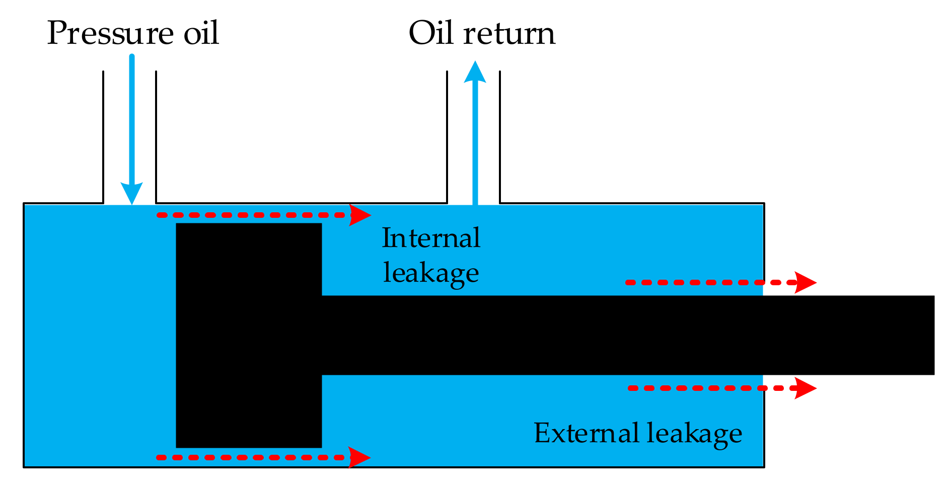
Considering there is no such thing as an absolutely perfect system without degradation, fault-free modeling of the system accounts for leaky fluid resistances, stuck fluid resistances, etc. To simulate and inject faults, only the pertinent resistive element parameters need to be altered.

Minor, general, serious, and deadly faults can be classified based on the degree of degradation of faults, and abrupt and progressive faults based on the degree of progression of faults. Table 3 shows that faults of types A, B, and C are studied in this study. To describe the system’s operational state, define the Boolean logic variable $\beta$:

$$\beta =[\mathrm{A},\mathrm{B},\mathrm{C}] (\mathrm{A}/\mathrm{B}/\mathrm{C}=0 or 1)$$

(11)

For example, $\beta =[0,0,1]$ means that only type C fault exist and no type A and B.

Table 3. Fault type and corresponding parameters.

Fault Type Number	Components Involved	Meaning
A	$R_{In-l}$	Internal leakage of actuator
B	$R_{Ex-l}$	External leakage of actuator
C	$R_{PA}$$R_{PB}$$R_{AT}$$R_{BT}$	Landing gear selector valve stuck

Table 3. Fault type and corresponding parameters.

Fault Type Number	Components Involved	Meaning
A	$R_{In-l}$	Internal leakage of actuator
B	$R_{Ex-l}$	External leakage of actuator
C	$R_{PA}$$R_{PB}$$R_{AT}$$R_{BT}$	Landing gear selector valve stuck

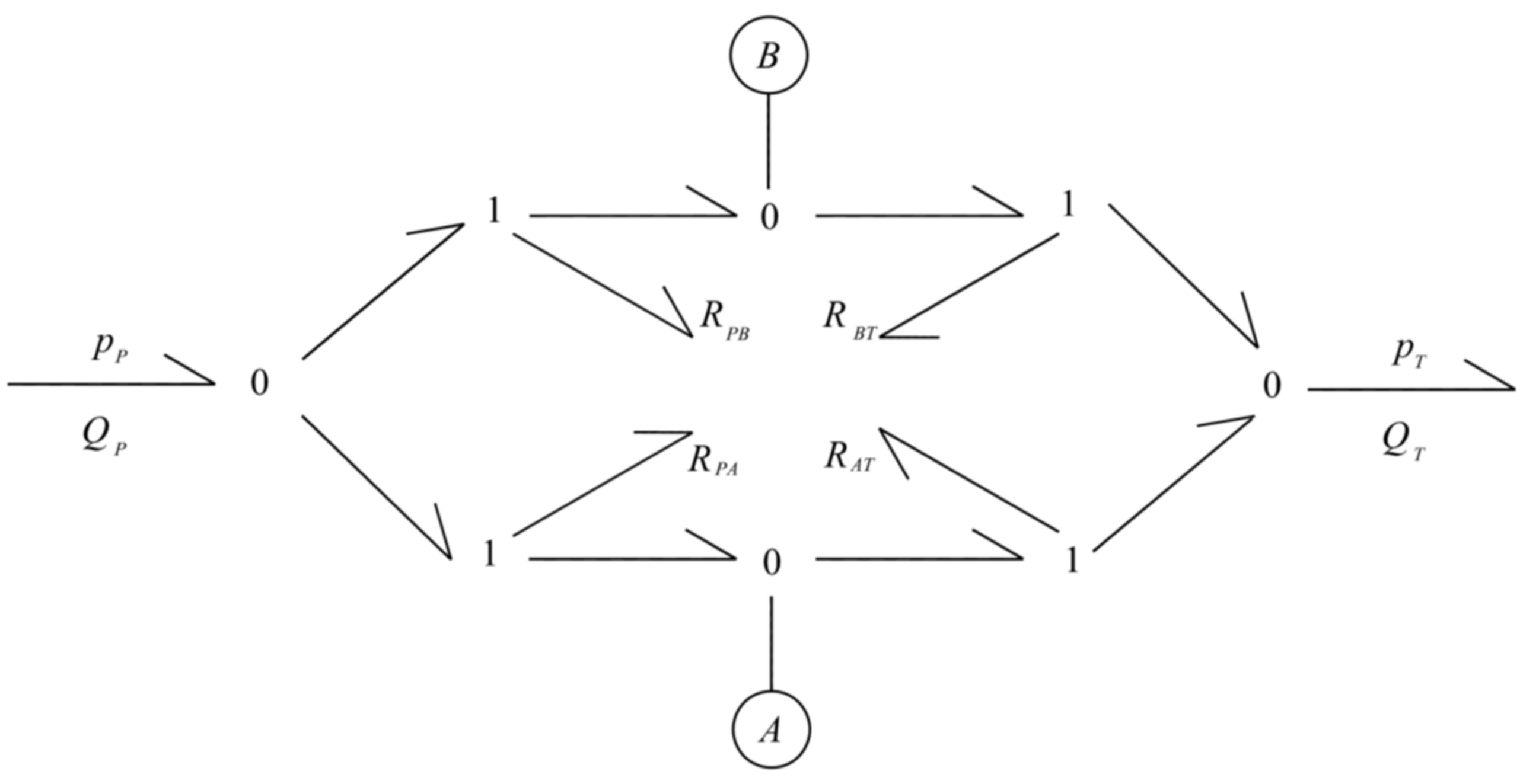
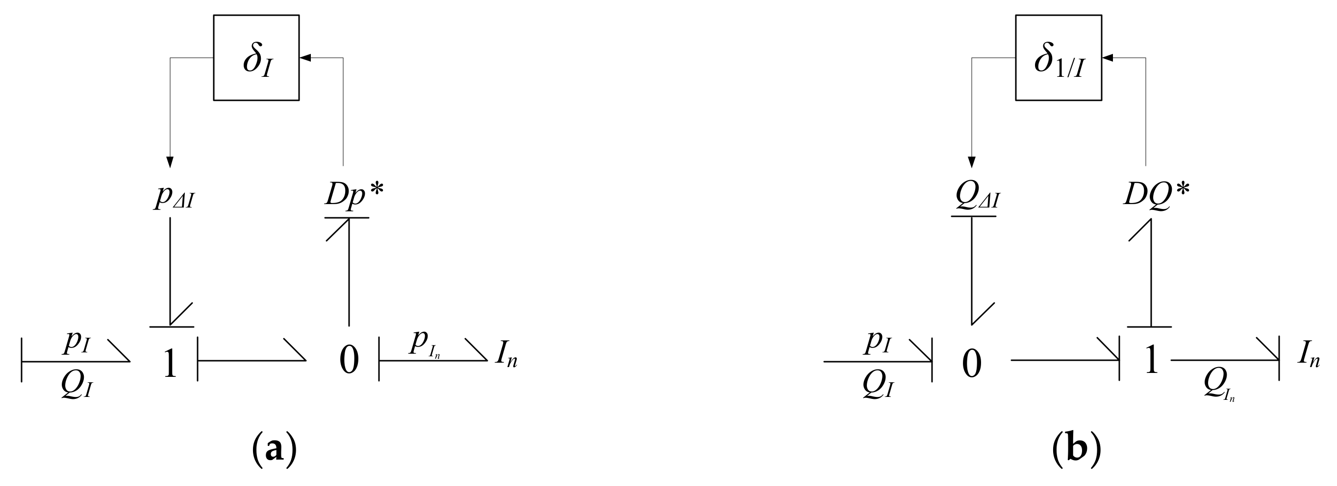
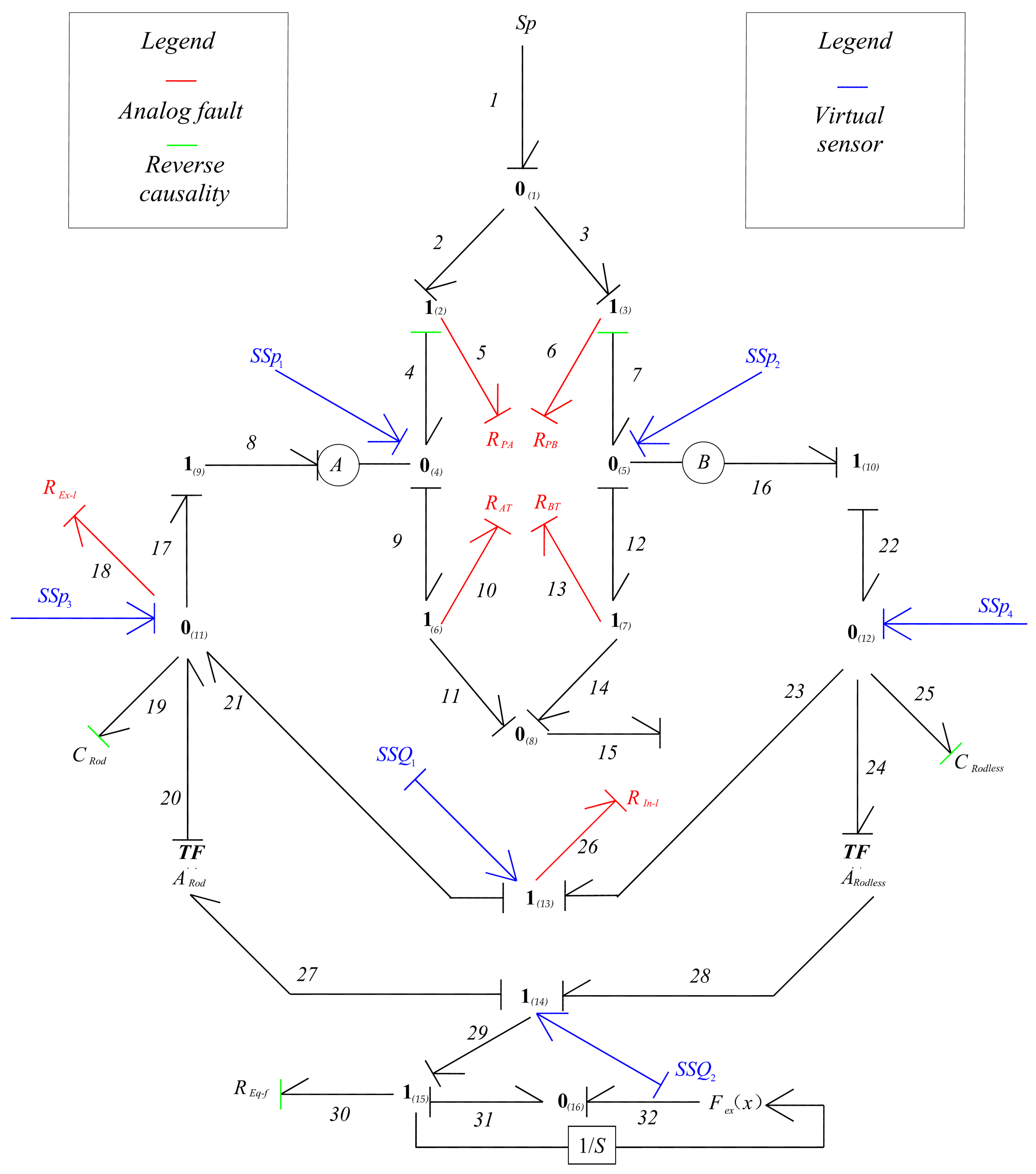
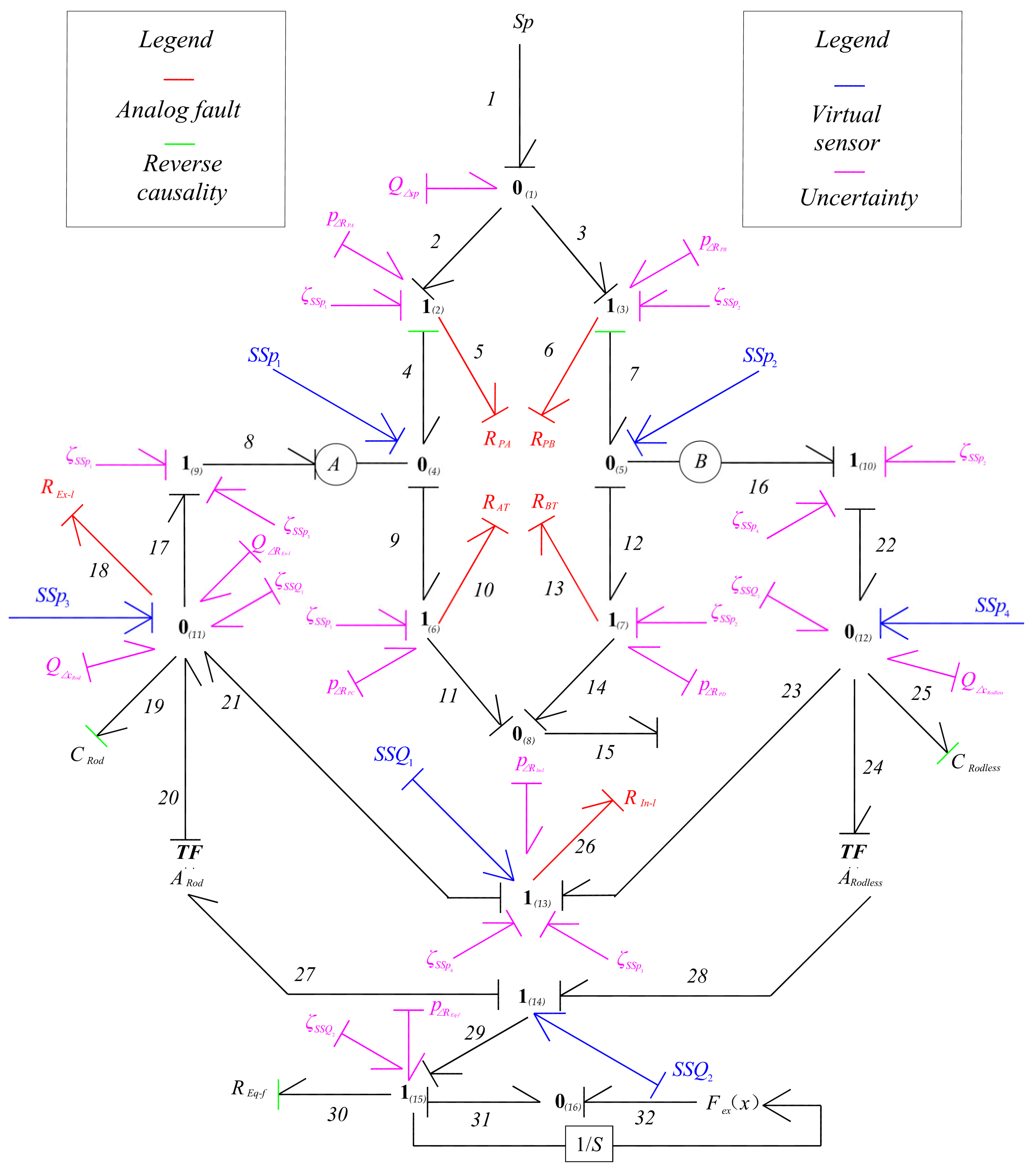
ARR at the co-potential node (0-node) can be summarized as “Same potential variable divides the flow variable”, and at the co-flow node (1-node) can be summarized as “Same flow variable divides the potential variable”:

$$0-\mathrm{node}:\left\{\begin{array}{l}{p}_1=p_2=p_3=\cdots p_n\\ \mathrm{ARR}={\displaystyle \sum _{i=1}^n{\alpha }_i{Q}_i}\end{array}\right. i=1,2,3,\cdots n$$

(12)

$$1-\mathrm{node}:\left\{\begin{array}{l}{Q}_1=Q_2=Q_3=\cdots Q_n\\ \mathrm{ARR}={\displaystyle \sum _{i=1}^n{\alpha }_i{p}_i}\end{array}\right.i=1,2,3,\cdots n$$

(13)

where $n$ is the node’s bond excluding the virtual sensor; ${\alpha }_i$ is the power flow coefficient, for the bond with the half-arrow pointing to the node ${\alpha }_i=1$ and for the bond with the half-arrow departing from the node ${\alpha }_i=-1$.

According to Figure 5, analytical redundancy relations (ARRs) and residuals $r_i$ are obtained.

ARR₁ for node$0_{(4)}$:

$$0_{(4)}-\mathrm{node}:\left\{\begin{array}{l}{p}_4=p_8=p_9\\ {\mathrm{ARR}}_1=Q_4+Q_8-Q_9=0\end{array}\right.$$

(14)

$$\left\{\begin{array}{l}{Q}_4=Q_2=Q_5=\frac{p_5}{R_{PA}}=\frac{p_2-p_4}{R_{PA}}=\frac{Sp-SS{p}_1}{R_{PA}}\\ Q_8=Q_{17}=Q_{21}+Q_{20}-Q_{19}-Q_{18}=SS{Q}_1+\frac{SS{Q}_2}{A_{Rod}}-C_{Rod}\frac{d(SS{p}_3)}{dt}-\frac{SS{p}_3}{R_{Ex-l}}\\ Q_9=Q_{10}=Q_{11}=\frac{p_{10}}{R_{AT}}=\frac{p_9-p_{11}}{R_{AT}}=\frac{SS{p}_1-p_T}{R_{AT}}\end{array}\right.$$

(15)

$$r_1=\frac{Sp-SS{p}_1}{R_{PA}}+SS{Q}_1+\frac{SS{Q}_2}{A_{Rod}}-C_{Rod}\frac{d(SS{p}_3)}{dt}-\frac{SS{p}_3}{R_{Ex-l}}-\frac{SS{p}_1-p_T}{R_{AT}}$$

(16)

ARR₂ for node$0_{(5)}$:

$$0_{(5)}-\mathrm{node}:\left\{\begin{array}{l}{p}_7=p_{12}=p_{16}\\ {\mathrm{ARR}}_2=Q_7-Q_{12}-Q_{16}=0\end{array}\right.$$

(17)

$$\left\{\begin{array}{l}{Q}_7=Q_3=Q_6=\frac{p_6}{R_{PB}}=\frac{p_3-p_7}{R_{PB}}=\frac{Sp-SS{p}_2}{R_{PB}}\\ Q_{12}=Q_{13}=Q_{14}=\frac{p_{13}}{R_{BT}}=\frac{p_{12}-p_{14}}{R_{BT}}=\frac{SS{p}_2-p_T}{R_{BT}}\\ Q_{16}=Q_{22}=Q_{23}+Q_{24}+Q_{25}=SS{Q}_1+A_{Rodless}SS{Q}_2+C_{Rodless}\frac{d(SS{p}_4)}{dt}\end{array}\right.$$

(18)

$$r_2=\frac{Sp-SS{p}_2}{R_{PB}}-\frac{SS{p}_2-p_T}{R_{BT}}-SS{Q}_1-A_{Rodless}SS{Q}_2-C_{Rodless}\frac{d(SS{p}_4)}{dt}$$

(19)

ARR₃ for node$1_{(13)}$:

$$1_{(13)}-\mathrm{node}:\left\{\begin{array}{l}{Q}_{23}=Q_{21}=Q_{26}\\ {\mathrm{ARR}}_3=p_{23}-p_{21}-p_{26}=0\end{array}\right.$$

(20)

$$\left\{\begin{array}{l}{p}_{21}=SS{p}_3\\ p_{23}=SS{p}_4\\ p_{26}=R_{In-l}SS{Q}_1\end{array}\right.$$

(21)

$$r_3=SS{p}_4-SS{p}_3-R_{In-l}SS{Q}_1$$

(22)

ARR₄ for node$1_{(14)}$:

$$1_{(14)}-\mathrm{node}:\left\{\begin{array}{l}{Q}_{27}=Q_{28}=Q_{29}\\ {\mathrm{ARR}}_4=p_{28}-p_{27}-p_{29}=0\end{array}\right.$$

(23)

$$\left\{\begin{array}{l}{p}_{27}=\frac{p_{20}}{A_{Rod}}=\frac{SS{p}_3}{A_{Rod}}\\ p_{28}=A_{Rodless}{p}_{24}=A_{Rodless}SS{p}_4\\ p_{29}=p_{30}+p_{31}=R_{Eq-f}SS{Q}_2+F_{ex}(x)\end{array}\right.$$

(24)

$$r_4=A_{Rodless}SS{p}_4-\frac{SS{p}_3}{A_{Rod}}-R_{Eq-f}SS{Q}_2-F_{ex}(x)$$

(25)

Define the residual $r_i$, which has no dimensions of its own. In accordance with the correlation between parameters and ARRs, the fault signature matrix (FSM) is obtained. FSM is shown in Table 4. For the elements $M_{mn}$, $m$ is the number of rows, $n$ is the number of columns in the matrix, and the relationship is:

$$M_{mn}=\left\{\begin{array}{l}1 Parameter\in {\mathrm{ARR}}_i(r_i)\\ 0 Parameter\notin {\mathrm{ARR}}_i(r_i)\end{array}\right.$$

(26)

For any parameter corresponding to a lateral quantity such as $M_{1n}=[M_{11},M_{12},M_{13},\cdots ,M_{1n}]$, detectability $D_b$ and isolatability $I_b$ are:

$$D_b=\left\{\begin{array}{l}1 M_{1n}=[M_{11},M_{12},M_{13},\cdots ,M_{1n}]\ne [0,\cdots ,0]\\ 0 M_{1n}=[M_{11},M_{12},M_{13},\cdots ,M_{1n}]=[0,\cdots ,0]\end{array}\right.$$

(27)

$$I_b=\left\{\begin{array}{l}1 M_{1n}=[M_{11},M_{12},M_{13},\cdots ,M_{1n}] is unique\\ 0 M_{1n}=[M_{11},M_{12},M_{13},\cdots ,M_{1n}] is not unique\end{array}\right.$$

(28)

$$\left\{\begin{array}{l}{r}_i={\mathrm{ARR}}_i=0 No fault\\ r_i={\mathrm{ARR}}_i\ne 0 Faulty\end{array}\right.$$

(29)

When a parameter in the FSM deviates from the nominal value, the detectability indicates that the fault can be detected, but not all parameters are separable. The FSM’s non-zero elements have been identified by a distinctive hue that denotes the following:

Red: residual elements in the matrix that are not 0. It means that the residual in this column contains the corresponding parameter on the left side.

Blue: detectability element that is not 0. It means that the parameters in this line have the detectability of faults.

Green: isolability element that is not 0. It means that the parameters in this line have fault isolation.

Table 4. Fault signature matrix of landing gear R/E hydraulic system.

Parameter	r1	r2	r3	r4	Db	Ib
$Sp$	1	1	0	0	1	0
$R_{Ex-l}$	1	0	0	0	1	0
$R_{In-l}$	0	0	1	0	1	1
$R_{PA}$	1	0	0	0	1	0
$R_{PB}$	0	1	0	0	1	0
$R_{AT}$	1	0	0	0	1	0
$R_{BT}$	0	1	0	0	1	0
$p_T$	1	1	0	0	1	0
$C_{Rod}$	1	0	0	0	1	0
$C_{Rodless}$	0	1	0	0	1	0
$A_{Rod}$	1	0	0	1	1	1
$A_{Rodless}$	0	1	0	1	1	1
$R_{Eq-f}$	0	0	0	1	1	0
$F_{ex}(x)$	0	0	0	1	1	0

Table 4. Fault signature matrix of landing gear R/E hydraulic system.

Parameter	r1	r2	r3	r4	Db	Ib
$Sp$	1	1	0	0	1	0
$R_{Ex-l}$	1	0	0	0	1	0
$R_{In-l}$	0	0	1	0	1	1
$R_{PA}$	1	0	0	0	1	0
$R_{PB}$	0	1	0	0	1	0
$R_{AT}$	1	0	0	0	1	0
$R_{BT}$	0	1	0	0	1	0
$p_T$	1	1	0	0	1	0
$C_{Rod}$	1	0	0	0	1	0
$C_{Rodless}$	0	1	0	0	1	0
$A_{Rod}$	1	0	0	1	1	1
$A_{Rodless}$	0	1	0	1	1	1
$R_{Eq-f}$	0	0	0	1	1	0
$F_{ex}(x)$	0	0	0	1	1	0

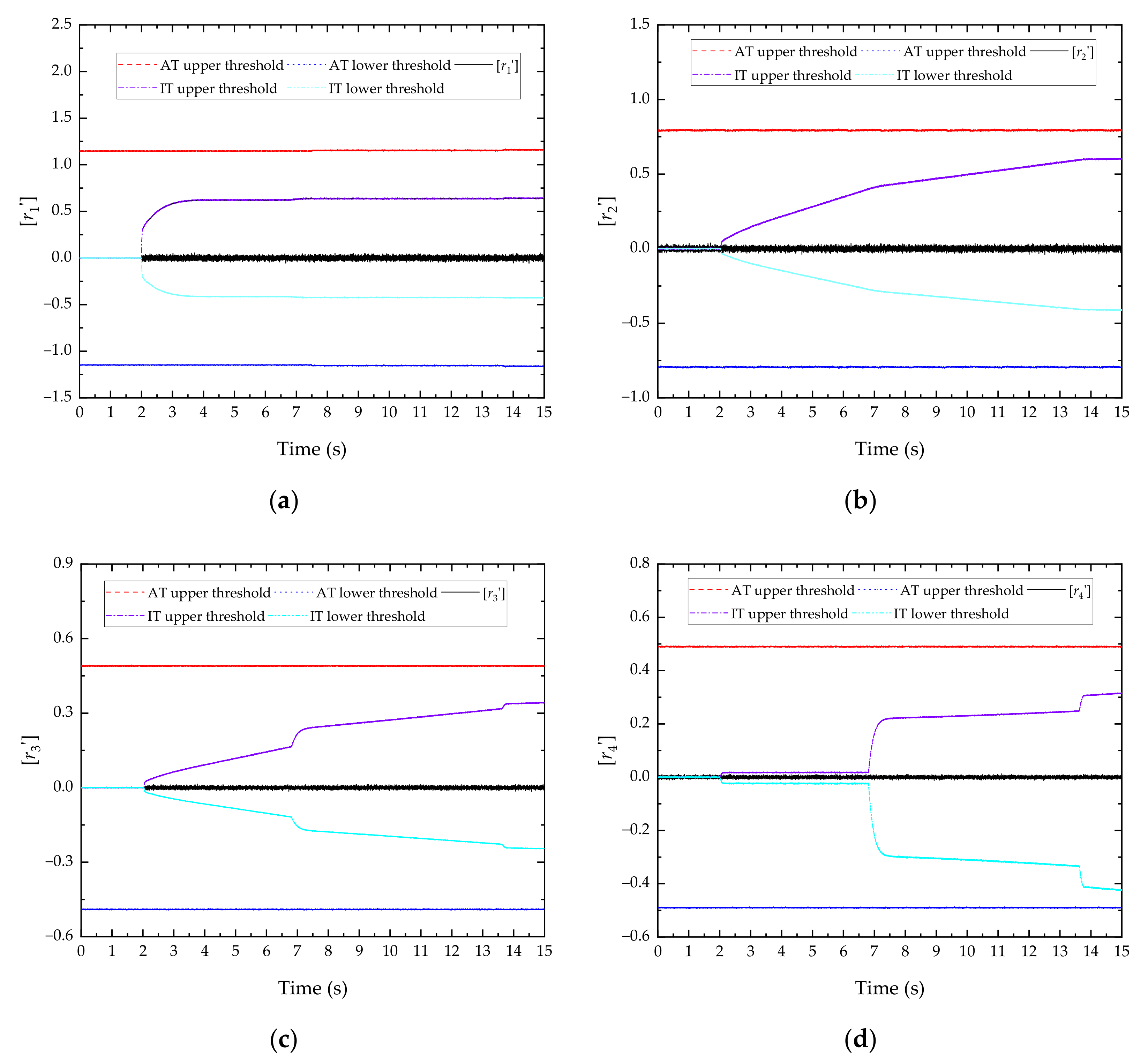
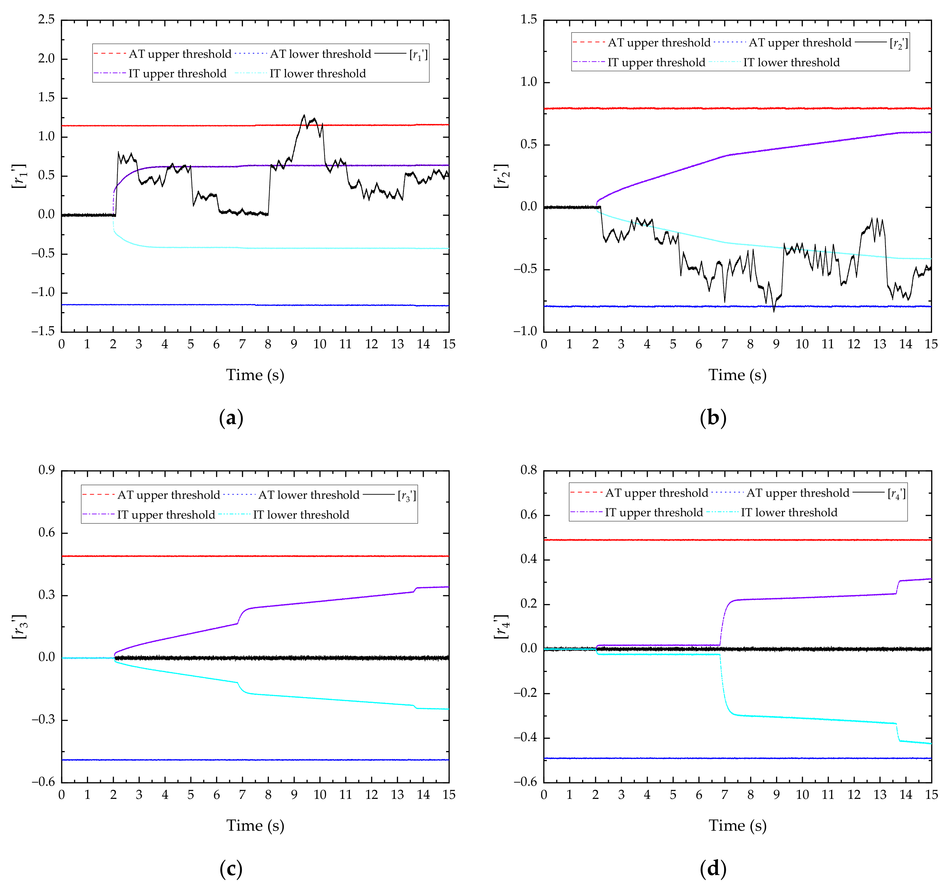
4.2. Interval Analytical Redundancy Relations Method

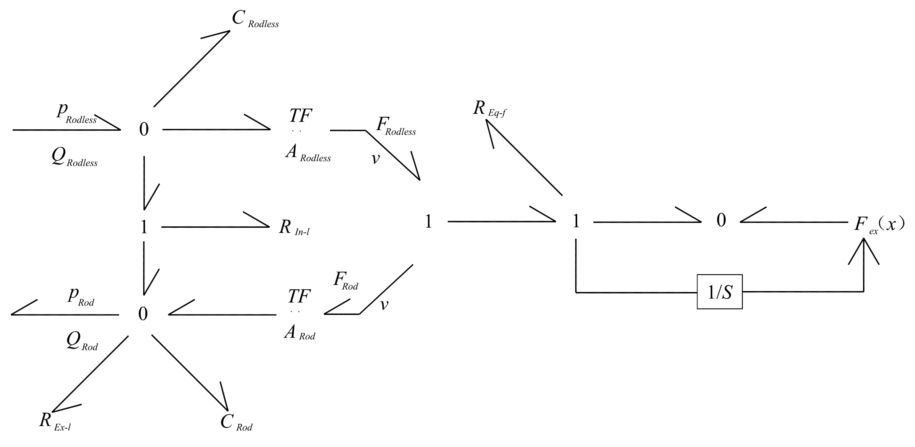
Based on the traditional analytical redundancy relation method, the interval analytical redundancy relation method in Section 3 is introduced. According to Figure 13, the residual derivation under the interval analytical redundancy relations is performed.

Taking residual $r_1$ as an example, the new residual $r_1{}^{\prime }$ after considering the negative effects of various uncertainties of the system is

$$\begin{array}{l}{r}_1{}^{\prime }=\frac{(1+{\delta }_{Sp})Sp-(SS{p}_1+{\zeta }_{SS{p}_1})}{(1+{\delta }_{R_{PA}})R_{PA}}+(SS{Q}_1+{\zeta }_{SS{Q}_1})+\frac{SS{Q}_2+{\zeta }_{SS{Q}_2}}{(1+{\delta }_{A_{Rod}})A_{Rod}}\\ -(1+{\delta }_{C_{Rod}})C_{Rod}\frac{d(SS{p}_3+{\zeta }_{SS{p}_3})}{dt}-\frac{SS{p}_3+{\zeta }_{SS{p}_3}}{(1+{\delta }_{R_{Ex-l}})R_{Ex-l}}-\frac{(SS{p}_1+{\zeta }_{SS{p}_1})-(1+{\delta }_{p_T})p_T}{(1+{\delta }_{R_{AT}})R_{AT}}\end{array}$$

(30)

wherein $\delta$ is the corresponding of the parameter, and $\zeta$ is the uncertainty of the measured value of the sensor.

After considering the interval analytic redundancy method, $r_1{}^{\prime }$ becomes $\left[r_1{}^{\prime }\right]$.

$$\begin{array}{ll}\left[r_1{}^{\prime }\right]=& \left[\underset{\_}{r_1{}^{\prime }},\overline{r_1{}^{\prime }}\right]=\frac{(1+\left[{\delta }_{Sp}\right])Sp-(SS{p}_1+\left[{\zeta }_{SS{p}_1}\right])}{(1+\left[{\delta }_{R_{PA}}\right])R_{PA}}+(SS{Q}_1+\left[{\zeta }_{SS{Q}_1}\right])+\frac{SS{Q}_2+\left[{\zeta }_{SS{Q}_2}\right]}{(1+\left[{\delta }_{A_{Rod}}\right])A_{Rod}}\\ & -(1+\left[{\delta }_{C_{Rod}}\right])C_{Rod}\frac{d(SS{p}_3+\left[{\zeta }_{SS{p}_3}\right])}{dt}-\frac{SS{p}_3+\left[{\zeta }_{SS{p}_3}\right]}{(1+\left[{\delta }_{R_{Ex-l}}\right])R_{Ex-l}}-\frac{(SS{p}_1+\left[{\zeta }_{SS{p}_1}\right])-(1+\left[{\delta }_{p_T}\right])p_T}{(1+\left[{\delta }_{R_{AT}}\right])R_{AT}}\end{array}$$

(31)

$\left[r_2{}^{\prime }\right]$, $\left[r_3{}^{\prime }\right]$, $\left[r_4{}^{\prime }\right]$ can be obtained according to the same method:

$$\{\begin{array}{l}\left[r_2{}^{\prime }\right]=\left[\underset{\_}{r_2{}^{\prime }},\overline{r_2{}^{\prime }}\right]=\frac{(1+\left[{\delta }_{Sp}\right])Sp-(SS{p}_2+\left[{\zeta }_{SS{p}_2}\right])}{(1+\left[{\delta }_{R_{PB}}\right])R_{PB}}-\frac{(SS{p}_2+\left[{\zeta }_{SS{p}_2}\right])-(1+\left[{\delta }_{p_T}\right])p_T}{(1+\left[{\delta }_{R_{BT}}\right])R_{BT}}\\ -(SS{Q}_1+\left[{\zeta }_{SS{Q}_1}\right])-(1+\left[{\delta }_{A_{Rodless}}\right])A_{Rodless}(SS{Q}_2+\left[{\zeta }_{SS{Q}_2}\right])-(1+\left[{\delta }_{C_{Rodless}}\right])C_{Rodless}\frac{d(SS{p}_4+\left[{\zeta }_{SS{p}_4}\right])}{dt}\\ \left[r_3{}^{\prime }\right]=\left[\underset{\_}{r_3{}^{\prime }},\overline{r_3{}^{\prime }}\right]=(SS{p}_4+\left[{\zeta }_{SS{p}_4}\right])-(SS{p}_3+\left[{\zeta }_{SS{p}_3}\right])-(1+{\delta }_{R_{In-l}})R_{In-l}(SS{Q}_1+\left[{\zeta }_{SS{Q}_1}\right])\\ \left[r_4{}^{\prime }\right]=\left[\underset{\_}{r_4{}^{\prime }},\overline{r_4{}^{\prime }}\right]=(1+\left[{\delta }_{A_{Rodless}}\right])A_{Rodless}(SS{p}_4+\left[{\zeta }_{SS{p}_4}\right])-\frac{SS{p}_3+\left[{\zeta }_{SS{p}_3}\right]}{(1+\left[{\delta }_{A_{Rod}}\right])A_{Rod}}\\ -(1+\left[{\delta }_{R_{Eq-f}}\right])R_{Eq-f}(SS{Q}_2+\left[{\zeta }_{SS{Q}_2}\right])-(1+\left[{\delta }_{F_{ex}(x)}\right])F_{ex}(x)\end{array}$$

(32)

See

Table 5. Interval values in Equations (37) and (38).

Parameter Uncertainty	Measurement Uncertainty
$\left[{\delta }_{Sp}\right]=\left[-\Delta S{p}_l/Sp,\Delta S{p}_r/Sp\right]$	$\left[{\zeta }_{SS{p}_1}\right]=\left[-\Delta SS{p}_{1_l},\Delta SS{p}_{1_r}\right]$
$\left[{\delta }_{R_{PA}}\right]=\left[-\Delta R_{P{A}_l}/R_{PA},\Delta R_{P{A}_r}/R_{PA}\right]$
$\left[{\delta }_{A_{Rod}}\right]=\left[-\Delta A_{Ro{d}_l}/A_{Rod},\Delta A_{Ro{d}_r}/A_{Rod}\right]$	$\left[{\zeta }_{SS{p}_2}\right]=\left[-\Delta SS{p}_{2_l},\Delta SS{p}_{2_r}\right]$
$\left[{\delta }_{C_{Rod}}\right]=\left[-\Delta C_{Ro{d}_l}/C_{Rod},\Delta C_{Ro{d}_r}/C_{Rod}\right]$
$\left[{\delta }_{R_{Ex-l}}\right]=\left[-\Delta R_{Ex-l_l}/R_{Ex-l},\Delta R_{Ex-l_r}/R_{Ex-l}\right]$	$\left[{\zeta }_{SS{p}_3}\right]=\left[-\Delta SS{p}_{3_l},\Delta SS{p}_{3_r}\right]$
$\left[{\delta }_{R_{AT}}\right]=\left[-\Delta R_{A{T}_l}/R_{AT},\Delta R_{A{T}_r}/R_{AT}\right]$
$\left[{\delta }_{p_T}\right]=\left[-\Delta p_{T_l}/p_T,\Delta p_{T_r}/p_T\right]$	$\left[{\zeta }_{SS{p}_4}\right]=\left[-\Delta SS{p}_{4_l},\Delta SS{p}_{4_r}\right]$
$\left[{\delta }_{R_{In-l}}\right]=\left[-\Delta R_{In-l_l}/R_{In-l},\Delta R_{In-l_r}/R_{In-l}\right]$
$\left[{\delta }_{R_{PB}}\right]=\left[-\Delta R_{P{B}_l}/R_{PB},\Delta R_{P{B}_r}/R_{PB}\right]$	$\left[{\zeta }_{SS{Q}_1}\right]=\left[-\Delta SS{Q}_{1_l},\Delta SS{Q}_{1_r}\right]$
$\left[{\delta }_{R_{BT}}\right]=\left[-\Delta R_{B{T}_l}/R_{BT},\Delta R_{B{T}_r}/R_{BT}\right]$
$\left[{\delta }_{C_{Rodless}}\right]=\left[-\Delta C_{Rodles{s}_l}/C_{Rodless},\Delta C_{Rodles{s}_r}/C_{Rodless}\right]$	$\left[{\zeta }_{SS{Q}_2}\right]=\left[-\Delta SS{Q}_{2_l},\Delta SS{Q}_{2_r}\right]$
$\left[{\delta }_{A_{Rodless}}\right]=\left[-\Delta A_{Rodles{s}_l}/A_{Rodless},\Delta A_{Rodles{s}_r}/A_{Rodless}\right]$
$\left[{\delta }_{R_{Eq-f}}\right]=\left[-\Delta R_{Eq-f_l}/R_{Eq-f},\Delta R_{Eq-f_r}/R_{Eq-f}\right]$
$\left[{\delta }_{F_{ex}(x)}\right]=\left[-\Delta F_{ex}{(x)}_l/F_{ex}(x),\Delta F_{ex}{(x)}_r/F_{ex}(x)\right]$

for interval values in Equations (37) and (38).

There are differential terms $d(SS{p}_3+\left[{\zeta }_{SS{p}_3}\right]/dt$ and $d(SS{p}_4+\left[{\zeta }_{SS{p}_4}\right])/dt$ in Equations (37) and (38), respectively. It is necessary to further calculate the first-order differential and the second-order differential by the backward differential method.

$$\left\{\begin{array}{l}\frac{d(SS{p}_3+\left[{\zeta }_{SS{p}_3}\right])}{dt}=\frac{d(SS{p}_3)}{dt}+\left[{\zeta }_{SS{p}_3}\right]\\ \frac{d(SS{p}_4+\left[{\zeta }_{SS{p}_4}\right])}{dt}=\frac{d(SS{p}_4)}{dt}+\left[{\zeta }_{SS{p}_4}\right]\end{array}\right.\left\{\begin{array}{l}\frac{d^2(SS{p}_3+\left[{\zeta }_{SS{p}_3}\right])}{d{t}^2}=\frac{d^2(SS{p}_3)}{d{t}^2}+\left[{\zeta }_{SS{p}_3}\right]\\ \frac{d^2(SS{p}_4+\left[{\zeta }_{SS{p}_4}\right])}{d{t}^2}=\frac{d^2(SS{p}_4)}{d{t}^2}+\left[{\zeta }_{SS{p}_4}\right]\end{array}\right.$$

(33)

Therefore, the uncertainty terms $\left[u_1\right]$, $\left[u_2\right]$, $\left[u_3\right]$, $\left[u_4\right]$ corresponding to $\left[r_1{}^{\prime }\right]$, $\left[r_2{}^{\prime }\right]$, $\left[r_3{}^{\prime }\right]$, $\left[r_4{}^{\prime }\right]$ can be obtained.

$$\left\{\begin{array}{l}\left[u_1\right]=\frac{(1+\left[{\delta }_{Sp}\right])Sp-(SS{p}_1+\left[{\zeta }_{SS{p}_1}\right])}{(1+\left[{\delta }_{R_{PA}}\right])R_{PA}}+\left[{\zeta }_{SS{Q}_1}\right]+\frac{SS{Q}_2+\left[{\zeta }_{SS{Q}_2}\right]}{(1+\left[{\delta }_{A_{Rod}}\right])A_{Rod}}\hfill \\ \hspace{1em}\hspace{1em}-(1+\left[{\delta }_{C_{Rod}}\right])C_{Rod}\left[{\zeta }_{SS{p}_3}\right]-\frac{SS{p}_3+\left[{\zeta }_{SS{p}_3}\right]}{(1+\left[{\delta }_{R_{Ex-l}}\right])R_{Ex-l}}-\frac{(SS{p}_1+\left[{\zeta }_{SS{p}_1}\right])-(1+\left[{\delta }_{p_T}\right])p_T}{(1+\left[{\delta }_{R_{AT}}\right])R_{AT}}\hfill \\ \left[u_2\right]=\frac{(1+\left[{\delta }_{Sp}\right])Sp-(SS{p}_2+\left[{\zeta }_{SS{p}_2}\right])}{(1+\left[{\delta }_{R_{PB}}\right])R_{PB}}-\frac{(SS{p}_2+\left[{\zeta }_{SS{p}_2}\right])-(1+\left[{\delta }_{p_T}\right])p_T}{(1+\left[{\delta }_{R_{BT}}\right])R_{BT}}\hfill \\ \hspace{1em}\hspace{1em}-\left[{\zeta }_{SS{Q}_1}\right]-(1+\left[{\delta }_{A_{Rodless}}\right])A_{Rodless}(SS{Q}_2+\left[{\zeta }_{SS{Q}_2}\right])-(1+\left[{\delta }_{C_{Rodless}}\right])C_{Rodless}\left[{\zeta }_{SS{p}_4}\right]\hfill \\ \left[u_3\right]=\left[{\zeta }_{SS{p}_4}\right]-\left[{\zeta }_{SS{p}_3}\right]-{\delta }_{R_{In-l}}(SS{Q}_1+\left[{\zeta }_{SS{Q}_1}\right])-R_{In-l}\left[{\zeta }_{SS{Q}_1}\right])\hfill \\ \left[u_4\right]=\left[{\delta }_{A_{Rodless}}\right]A_{Rodless}(SS{p}_4+\left[{\zeta }_{SS{p}_4}\right])+A_{Rodless}\left[{\zeta }_{SS{p}_4}\right]-\frac{SS{p}_3+\left[{\zeta }_{SS{p}_3}\right]}{(1+\left[{\delta }_{A_{Rod}}\right])A_{Rod}}\hfill \\ \hspace{1em}\hspace{1em}-\left[{\delta }_{R_{Eq-f}}\right]R_{Eq-f}(SS{Q}_2+\left[{\zeta }_{SS{Q}_2}\right])-R_{Eq-f}\left[{\zeta }_{SS{Q}_2}\right]-\left[{\delta }_{F_{ex}\left(x\right)}\right]F_{ex}\left(x\right)\hfill \end{array}\right.$$

(34)

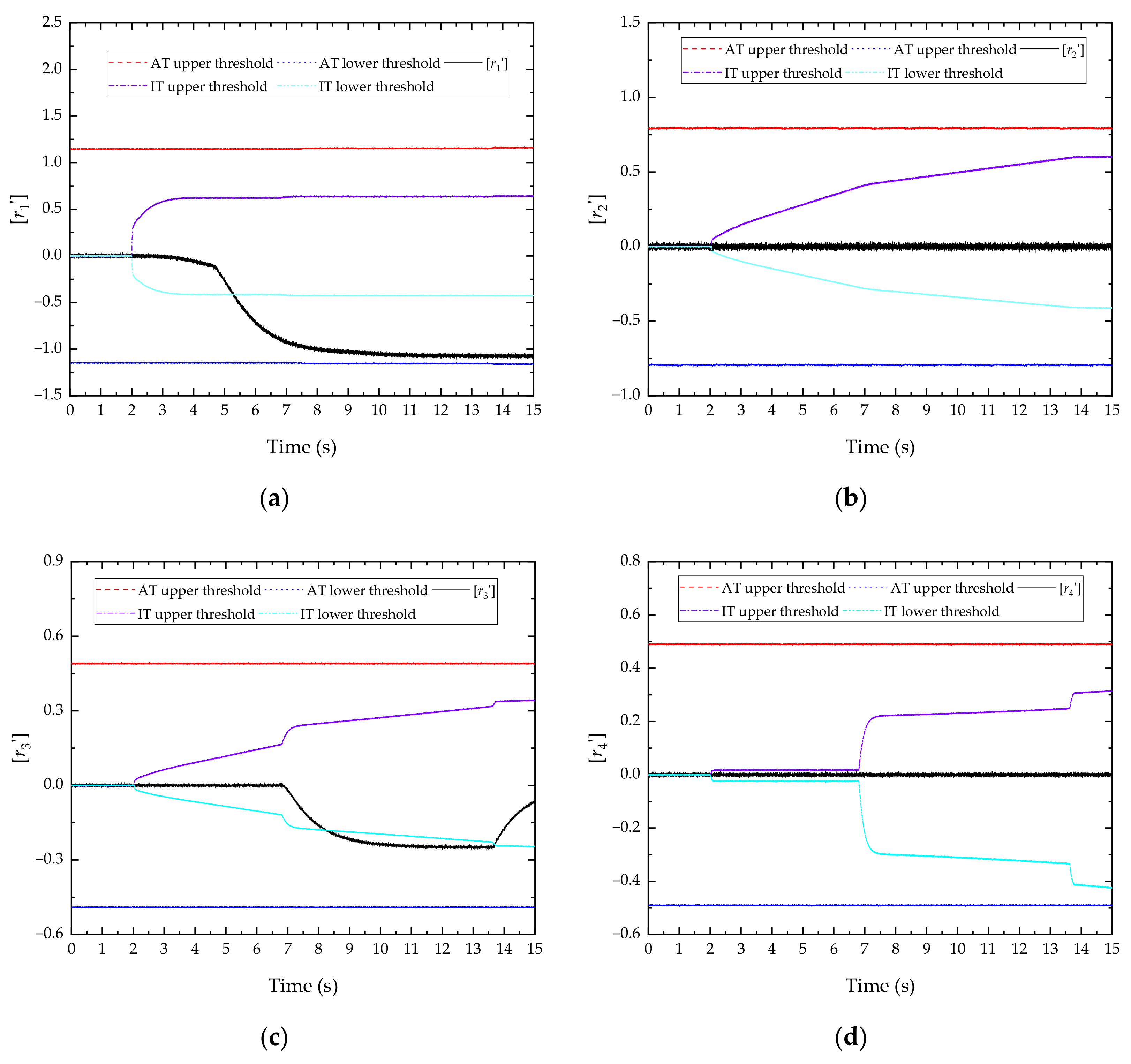
4.3. Diagnostic Thresholds and Data Acquisition

Positive, negative, or 0 residuals are possible. They have no dimensions and no physical significance. According to the literature [43,44], threshold deviation is defined as ${\epsilon }_i$, and the absolute value type threshold is:

$$\left\{\begin{array}{l}Upper threshold=r_i+{\epsilon }_i\\ Lower threshold=r_i-{\epsilon }_i\end{array}\right.$$

(35)

After considering the negative factors such as uncertainty ${\epsilon }_i=\Delta {\theta }_i\left|u_{{\theta }_i}\right|$, the absolute value type diagnostic threshold is:

$$\left\{\begin{array}{l}Upper threshold=r_i+\Delta {\theta }_i\left|u_{{\theta }_i}\right|\\ Lower threshold=r_i-\Delta {\theta }_i\left|u_{{\theta }_i}\right|\end{array}\right.$$

(36)

Table 6. The defined uncertainty value.

Parameter	Nominal Value	Absolute Value Type Uncertainty	Interval Type Uncertainty
$Sp$	$2.0685\times {10}^7 \mathrm{Pa} (3000 \mathrm{psi})$	$\pm 2.0685\times {10}^5$	$\left[-1.2000\times {10}^5,2.0685\times {10}^5\right]$
$R_{Ex-l}$	$9.35\times {10}^6 \mathrm{N}\cdot {\mathrm{s}/\mathrm{m}}^5$	$\pm 9.35\times {10}^4$	$\left[-7.50\times {10}^4,9.35\times {10}^4\right]$
$R_{In-l}$	$3.40\times {10}^6 \mathrm{N}\cdot {\mathrm{s}/\mathrm{m}}^5$	$\pm 3.40\times {10}^4$	$\left[-1.80\times {10}^4,3.40\times {10}^4\right]$
$R_{PA}$	$2.0\times {10}^{12} \mathrm{N}\cdot {\mathrm{s}/\mathrm{m}}^5$	$\pm 2.0\times {10}^{10}$	$\left[-0.5\times {10}^{10},2.0\times {10}^{10}\right]$
$R_{PB}$	$2.0\times {10}^{12} \mathrm{N}\cdot {\mathrm{s}/\mathrm{m}}^5$	$\pm 2.0\times {10}^{10}$	$\left[-0.5\times {10}^{10},2.0\times {10}^{10}\right]$
$R_{AT}$	$7.8\times {10}^9 \mathrm{N}\cdot {\mathrm{s}/\mathrm{m}}^5$	$\pm 7.8\times {10}^7$	$\left[-5.0\times {10}^7,7.8\times {10}^7\right]$
$R_{BT}$	$7.8\times {10}^9 \mathrm{N}\cdot {\mathrm{s}/\mathrm{m}}^5$	$\pm 7.8\times {10}^7$	$\left[-5.0\times {10}^7,7.8\times {10}^7\right]$
$p_T$	$2500 \mathrm{Pa}$	$\pm 25$	$\left[-5,25\right]$
$C_{Rod}$	$8.30\times {10}^{-13} {\mathrm{m}}^5/\mathrm{N}$	$\pm 8.30\times {10}^{-15}$	$\left[-3.60\times {10}^{-15},8.30\times {10}^{-15}\right]$
$C_{Rodless}$	$2.55\times {10}^{-13} {\mathrm{m}}^5/\mathrm{N}$	$\pm 2.55\times {10}^{-15}$	$\left[-1.50\times {10}^{-15},2.55\times {10}^{-15}\right]$
$A_{Rod}$	$0.0075 {\mathrm{m}}^2$	$\pm 7.50\times {10}^{-5}$	$\left[-4.50\times {10}^{-5},7.50\times {10}^{-5}\right]$
$A_{Rodless}$	$0.0125 {\mathrm{m}}^2$	$\pm 1.25\times {10}^{-4}$	$\left[-0.50\times {10}^{-4},1.25\times {10}^{-4}\right]$
$R_{Eq-f}$	$5.5\times {10}^{14} \mathrm{N}\cdot {\mathrm{s}/\mathrm{m}}^5$	$\pm 5.5\times {10}^{12}$	$\left[-3.0\times {10}^{12},5.5\times {10}^{12}\right]$
$F_{ex}(x)$	$2.22\times {10}^5 \mathrm{Pa}$	$\pm 2.22\times {10}^3$	$\left[-1.00\times {10}^3,2.22\times {10}^3\right]$

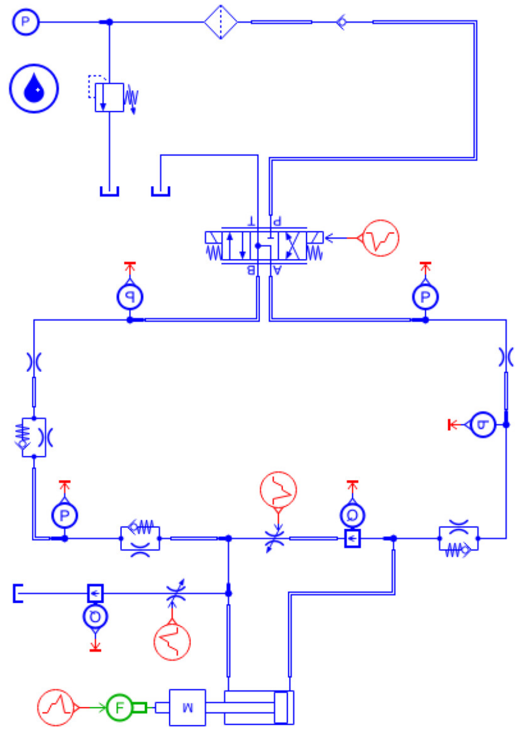
shows the defined uncertainty value, which is 1% of the original value. In addition, the measurement uncertainty error is defined as 0.1%. According to Figure 13, as illustrated in Figure 14, the diagnostic simulation model is created in the LMS Imagine. Lab AMESim simulation platform. It is the same sensor that is shown on the diagnostic bond graph.

The premise of the model-based simulation experiment is to prove the validity of the model. According to the professional maintenance manuals of Boeing and Airbus [45,46,47], as well as the computer-based training videos of maintenance professionals, under normal circumstances, the retraction time of landing gear is 7.5 s and the extension time is 10 s, which may vary slightly with different aircraft types. Technical manuals stipulate that actuation times cannot be changed more than 1 s. Actuator action is opposite to landing gear body action. When the retraction/extension actuator is extended, the landing gear retracts; when the actuator is retracted, the landing gear is retracted. The results of the diagnostic simulation model are shown in Figure 15. The retraction time of the actuator is from 2 s to 12.86 s, and the extension time of the actuator is from 2 s to 9.17 s.

As shown in Figure 15, the error bar sampling interval between the simulation effect curve and the absolute ideal curve is 0.001 s. Introducing [48] sum of squares of errors (SSE), mean-squared error (MSE), and model effect evaluation index $R^2$:

$$\left\{\begin{array}{l}SSE={\displaystyle \sum _{i=1}^n{(y_i-{\widehat{y}}_i)}^2}\\ MSE=\sqrt{\frac{1}{n}{\displaystyle \sum _{i=1}^n{(y_i-{\widehat{y}}_i)}^2}}\\ R^2=\frac{SSE-MSE}{SSE}\end{array}\right.$$

(37)

where $y_i$ and ${\widehat{y}}_i$ are the ideal value sampling points represented by the red curve and the simulation effect value sampling points represented by the black curve in Figure 15, respectively. MSE represents the error that cannot be explained by the model, so the larger the MSE, the worse the matching effect of the model. According to this principle, the larger $R^2$ is, the better the matching effect of the model. The value of $R^2$ can only be 0~1. Generally, if $R^2$ is lower than 0.5, the model will have poor effect. If $R^2$ is greater than 0.75, the model will perform well. In Figure 15a and b, the average $R^2$ is 0.7676, so the model matching is satisfactory.

5. Fault Case Analysis

5.1. Fault Free Operation of the System

Under MATLAB, the above output data was analyzed with the INTLAB interval operation toolkit. Its operation rules can be seen in [49]. The residuals $\left[r_1{}^{\prime }\right]$, $\left[r_2{}^{\prime }\right]$, $\left[r_3{}^{\prime }\right]$, $\left[r_4{}^{\prime }\right]$ under fault free operation are shown in Figure 16, wherein the diagnosis thresholds are of absolute type (AT) and interval type (IT), respectively.

Generally, the residual will continue to deteriorate in either a positive or negative direction. During the process of deterioration, it will not suddenly change from a positive value to a negative value. Through trial tests, the residual trend can be understood. Based on the diagnostic threshold method proposed above, the threshold can be appropriately reduced in the direction of the residual to further improve diagnostic sensitivity.

In civil aviation planned maintenance [50], there are generally three indicators to define the overall health of the aircraft, namely, flight hours/times of take-off and landing/calendar months. Which indicator is reached first will be used to implement the maintenance plan. According to these three indicators, the planned maintenance is divided into four levels: A/B/C/D. Boeing and Airbus series aircraft have obvious differences in the division of such indicators. Take Boeing series aircraft as an example. In general, A-level maintenance is 250 flight hours, B-level maintenance is cancelled and divided into A-level and C-level. C-level maintenance is 3200 flight hours, and D-level maintenance needs more than 10,000 flight hours. In the research system of this paper, its flight time does not exceed 3200 h and 1000 take-off and landing, that is, it does not exceed the time limit of C-level, and still focuses on route maintenance.

It can be seen from Figure 16 that the residuals $\left[r_1{}^{\prime }\right]$, $\left[r_2{}^{\prime }\right]$, $\left[r_3{}^{\prime }\right]$, and $\left[r_4{}^{\prime }\right]$ fluctuate up and down within a certain range of 0, and none exceed the diagnostic threshold. This indicates that no fault is detected during normal operation of the system, corresponding to $\beta =\left[0,0,0\right]$. Therefore, it can be proved that the uncertainty interference modeling and analysis method proposed in this paper is correct and feasible.

5.2. External and Internal Leakage of Actuator

As shown in Figure 17, leakage is one of the most prevalent failure types for actuators. Progressive failure is inherent in this process and cannot be avoided. In the description of the bathtub curve, it belongs to transition duration from the random failures period to the wearout period. Generally, it can be controlled by increasing tightness and performing regular inspections [51,52]. The red dotted line in Figure 17 represents the leakage flow. Leaks can be internal or external. External leaks occur between the piston rod and cylinder, while internal leaks occur between the cylinder and piston. Consider the extension of a piston rod as an example. Flow loss occurs between these two kinds of gaps when high-pressure hydraulic oil forces the piston out of the actuator cylinder.

As shown in Figure 14, the fault simulation method of external leakage is to connect the oil return chamber of the actuator with the oil tank, and control the leakage amount through the adjustable flow valve. By the same token, the internal leakage is simulated by connecting the pressure chamber of the actuator and the oil return chamber in series through the adjustable flow valve. The larger the opening of the adjustable flow valve, the larger the leakage, and the larger the corresponding leakage liquid resistance.

$$\left\{\begin{array}{l}{x}_{Ex-l}=0.05+0.05(t-2) 2\le t\le 15\\ x_{In-l}=0.02+0.01(t-2) 2\le t\le 15\end{array}\right.$$

(38)

where, $x_{Ex-l}$ and $x_{In-l}$ are the opening of the adjustable flow valve simulating external leakage and internal leakage, respectively. x′ range is 0 to 1.

Figure 18a shows that the residual $\left[r_1{}^{\prime }\right]$ exceeds the interval type (IT) lower threshold at 5.38 s, and external leakage of actuator cylinder is successfully diagnosed. However, the residual $\left[r_1{}^{\prime }\right]$ does not exceed the absolute type (AT) lower threshold not tested, resulting in missed diagnosis. Figure 18c shows that the residual $\left[r_3{}^{\prime }\right]$ exceeds the IT lower threshold at 8.32 s, and internal leakage of actuator cylinder is successfully diagnosed. However, the residual $\left[r_3{}^{\prime }\right]$ does not exceed the AT lower threshold not tested, resulting in missed diagnosis.

The residuals $\left[r_2{}^{\prime }\right]$ and $\left[r_4{}^{\prime }\right]$ in Figure 18b and d are basically no different from the normal operation of the system, which proves that the two threshold methods do not cause misdiagnosis. This also corresponds to $\beta =$ [1,1,0].

5.3. Landing Gear Selector Valve Reversing Stuck

Landing gear selector valve has 3 operational states [53]: Neutral, Left, and Right. Using the left as an example, we can see from the analysis above that at this moment, we do not take the liquid resistance $R_{PA}$ and $R_{BT}$ into consideration, they are constant fixed values, the fault diagnosis object is the liquid resistance $R_{PB}$ and $R_{AT}$. $R_{PB}$ corresponds to $\left[r_2{}^{\prime }\right]$, $R_{AT}$ corresponds to $\left[r_1{}^{\prime }\right]$. Shifting to the right reverses the object of research and control invariant liquid resistance.

Generally speaking, when jamming occurs, the friction between the valve core and the valve body of the reversing valve will not be equal or linearly increased anywhere, that is, it is considered as non-uniform friction. The causes may be high concentration of abrasive particles, poor cleanliness of oil, wear of mechanical structure, etc. This belongs to the wearout period in the bathtub curve and is a progressive failure. Therefore, the way to simulate the jamming is to adjust the reversing hydraulic resistance of the reversing valve in AMESim to change in a random sequence within a certain range. Among them, the random number sequences $a_{PB}$ and $a_{AT}$, respectively, are shown in

Table 7. Random sequence $a_{PB}$ and $a_{AT}$.

Time/s	2	3	4	5	6	7	8	9	10	11	12	13	14	15
Value of $a_{PB}$	1.0	1.5	1.2	1.6	2.1	2.6	1.7	2.4	1.0	1.7	2.1	1.0	2.2	1.8
Value of $a_{AT}$	1.0	1.7	1.3	1.6	1.1	1.0	1.0	1.6	1.7	1.2	1.0	1.3	1.5	1.2

.

$$\left\{\begin{array}{l}{R}_{PB}=2.0\times {10}^{12}\cdot a_{PB}\\ R_{AT}=7.8\times {10}^9\cdot a_{AT}\end{array}\right.$$

(39)

Figure 19a shows that the residual $\left[r_1{}^{\prime }\right]$ exceeds the IT upper threshold at least four times and the AT upper threshold only once. Figure 19b shows that the residual $\left[r_2{}^{\prime }\right]$ exceeds the IT lower threshold at least six times and the AT upper threshold only once. Both of them successfully detect the preset fault, but the IT has better sensitivity.

The residuals $\left[r_3{}^{\prime }\right]$ and $\left[r_4{}^{\prime }\right]$ in Figure 19b,d are basically no different from the normal operation of the system, which proves that the two threshold methods do not cause misdiagnosis. This also corresponds to $\beta =$ [0,0,1].

From the above, it can be seen that only the residuals in Figure 18a,c and Figure 19a,b deviate seriously from 0, that is, a fault is detected. There are many types of errors. The parameter uncertainty and measurement uncertainty studied above also belong to errors. In addition, take Figure 18a,c and Figure 19a,b as observation values, and the filtered image itself is the true value. The calculated relative error images are shown in Figures S1–S4, respectively.

6. Conclusions

Landing gear retraction/extension hydraulic system is a nonlinear dynamic system. In the research of fault diagnosis, it is unavoidable to consider the interference factors such as component parameter uncertainty and sensor measurement uncertainty. The advantage of the method proposed in this paper, which combines the linear fractional transformation technology of bond graphs and the interval analysis redundancy relations, is that it can effectively avoid or reduce the missed diagnosis and misdiagnosis caused by such interference factors. At the same time, through example analysis, the interval threshold obtained in this paper has higher detection accuracy and sensitivity than the traditional absolute threshold.

However, the limitation of this study is that it only stays at the level of fault detection, and there is less research on fault isolation after detection, that is, how to determine the type and location of faults after detection needs further research.

References

1. Boeing. Statistical Summary of Commercial Jet Airplane Accidents Worldwide Operations 1959–2017; Boeing Commercial Airplanes: Seattle, WA, USA, 2018. [Google Scholar]
2. Airbus. A Statistical Analysis of Commercial Aviation Accidents 1958–2018; Airbus S.A.S. 31707: Blagnac, France, 2019. [Google Scholar]
3. EASA. Annual Safety Review 2020; European Union Aviation Safety Agency: Cologne, Germany, 2020. [Google Scholar]
4. ICAO. State of Global Aviation Safety; International Civil Aviation Organization: Montréal, QC, Canada, 2019. [Google Scholar]
5. Yang, L.; Hu, Z.; He, Y. Prediction of wrinkle types in tube hydroforming under pulsating hydraulic pressure with axial feeding. Proc. Inst. Mech. Eng. Part C J. Mech. Eng. Sci. 2017, 231, 2810–2821. [Google Scholar]
6. Ouyang, X.; Gao, F.; Yang, H.; Wang, H. Two-dimensional stress analysis of the aircraft hydraulic system pipeline. Proc. Inst. Mech. Eng. Part G J. Aerosp. Eng. 2011, 226, 532–539. [Google Scholar] [CrossRef]
7. Han, X. Research on Lightweight Distributed Neural Network Technology for Fault Diagnosis. Master’s Thesis, Zhejiang University, Hangzhou, China, 2022. [Google Scholar]
8. Yang, Y. Aircraft Landing Gear Extension and Retraction Control System Diagnostics Prognostics and Health Management. Master’s Thesis, Cranfield University, London, UK, 2012. [Google Scholar]
9. Shao, W. Research on the FMECA and FTA of the Landing Gear System for a Certain Type of Aircraft in Failure Analysis. Master’s Thesis, Xihua University, Chengdu, China, 2019. [Google Scholar]
10. Ji, X. Simulation and Research on Electrical Characteristics of Retraction and Extension Faults of More Electric Aircraft’s Landing Gear. Master’s Thesis, Civil Aviation University of China, Tianjin, China, 2019. [Google Scholar]
11. Saucedo-Dorantes, J.J.; Delgado-Prieto, M.; Osornio-Rios, R.A.; Romero-Troncoso, R.J. Industrial Data-Driven Monitoring Based on Incremental Learning Applied to the Detection of Novel Faults. IEEE Trans. Ind. Inform. 2020, 16, 5985–5995. [Google Scholar] [CrossRef]
12. Prasad, C.D.; Nayak, P.K. Performance assessment of swarm-assisted mean error estimation-based fault detection technique for transmission line protection. Comput. Electr. Eng. 2018, 71, 115–128. [Google Scholar] [CrossRef]
13. Li, F.; Wu, Z.; Li, J.; Lai, Z.; Zhao, B.; Min, C. A Multi-Step CNN-Based Estimation of Aircraft Landing Gear Angles. Sensors 2021, 21, 8440. [Google Scholar] [CrossRef]
14. Chen, J.; Xu, Q.; Guo, Y.; Chen, R. Aircraft Landing Gear Retraction/Extension System Fault Diagnosis with 1-D Dilated Convolutional Neural Network. Sensors 2022, 22, 1367. [Google Scholar] [CrossRef]
15. Nasiri, S.; Khosravani, M.R.; Weinberg, K. Fracture mechanics and mechanical fault detection by artificial intelligence methods: A review. Eng. Fail. Anal. 2017, 81, 270–293. [Google Scholar] [CrossRef]
16. Hu, Z.; Zhao, G.; Li, F.; Zhou, D. Fault diagnosis for nonlinear dynamical system based on adaptive unknown input observer. Control. Decis. 2016, 31, 901–906. [Google Scholar]
17. Liu, Y.; Sun, C.; Chen, Y.; Lin, G. Design and application on sliding mode controller for roller microporous system based on disturbance observer. Forg. Stamp. Technol. 2022, 47, 116–120. [Google Scholar]
18. Xu, G.; Yu, Z.; Lu, N.; Lv, G. High-gain observer-based sliding mode control for hydraulic excavators. J. Harbin Eng. Univ. 2021, 42, 885–892. [Google Scholar]
19. Yu, Y.; Xiao, Y.; Zhu, C.; Tong, J. Sliding Mode Control of Crane Anti-sway Positioning Based on Kalman Filter. Control. Eng. China 2021, 28, 1049–1054. [Google Scholar]
20. Huang, Y.; Bai, M.; Zhang, Y. A novel multiple-outlier-robust Kalman filter. Front. Inf. Technol. Electron. Eng. 2022, 23, 422–437. [Google Scholar] [CrossRef]
21. Cui, Z.; Jing, B.; Jiao, X.; Yao, W.; Zhou, Y. Design of fault-tolerant integrated navigation system based on federated Kalman filter. J. Electron. Meas. Instrum. 2021, 35, 143–153. [Google Scholar]
22. Wang, S. Research on Dynamic State Estimation of Power System Eased on Kalman Filter. Master’s Thesis, North China Electric Power University, Beijing, China, 2020. [Google Scholar]
23. Gao, S.; Li, R.; Huang, Z. A Fault-tolerance Estimating Method for Ionosphere Corrections in Satellite Navigation System. Chin. J. Aeronaut. 2011, 24, 749–755. [Google Scholar] [CrossRef]
24. Shen, W.; Yuan, X.; Liu, M. Event-triggered Control for Hydraulic Position Tracking System with Extended State Observer. J. Mech. Eng. 2022, 58, 274–284. [Google Scholar]
25. Qin, D.; Jian, J.; Cheng, K.; Wu, B. Adaptive Starting Control of Dual Clutch Transmission Based on Extended State Observer and Sliding-mode Control. China J. Highw. Transp. 2021, 34, 39–50. [Google Scholar]
26. Daroogheh, N.; Meskin, N.; Khorasani, K. A Dual Particle Filter-Based Fault Diagnosis Scheme for Nonlinear Systems. IEEE Trans. Control. Syst. Technol. 2018, 26, 1317–1334. [Google Scholar] [CrossRef]
27. Tian, K. Research on the Technology of Prediction and Diagnosis of Equipment Fault in Satellite Ground Station System. Master’s Thesis, University of Electronic Science and Technology of China, Chengdu, China, 2021. [Google Scholar]
28. Mo, H.; Li, Y. Fault Diagnosis Based on Interval Analytic Redundancy Relation. J. Nanjing Univ. Aeronaut. Astronaut. 2021, 53, 972–980. [Google Scholar]
29. Wang, F.; Pazilai, M.; Zhang, B. Robust fault diagnosis and fault tolerant control based on bond graph. Electr. Meas. Instrum. 2019, 56, 124–128. [Google Scholar]
30. Djeziri, M.A.; Bouamama, B.O.; Merzouki, R. Modelling and robust FDI of steam generator using uncertain bond graph model. J. Process Control. 2009, 19, 149–162. [Google Scholar] [CrossRef]
31. Duan, S.; Li, Y.; Cao, Y.; Wang, X.; Li, X.; Zhao, Z. Health Assessment of Landing Gear Retraction/Extension Hydraulic System Based on Improved Risk Coefficient and FCE Model. Appl. Sci. 2022, 12, 5409. [Google Scholar] [CrossRef]
32. Song, J.; Li, J.; Wang, B. Boeing 737NG Aircraft System; Aviation Industry Press: Beijing, China, 2016; pp. 97–114. [Google Scholar]
33. Wei, J.; Chen, Z.; Lu, W.; Jia, C. Aircraft System; Tsinghua University Press: Beijing, China, 2016; pp. 409–416. [Google Scholar]
34. Wang, Z. Bond Graph Theory and Its Application in System Dynamics; Harbin Engineering University Press: Harbin, China, 2000; pp. 38–46. [Google Scholar]
35. Yin, Y. Dynamics and Reliability Analysis of Retraction of Landing Gear. Ph.D. Thesis, Nanjing University of Aeronautics and Astronautics, Nanjing, China, 2017. [Google Scholar]
36. Yin, Y.; Nie, H.; Wei, X.; Ni, H. Performance analysis of landing gear retraction and extension system under the influence of multiple factors. J. Beijing Univ. Aeronaut. Astronaut. 2015, 41, 953–960. [Google Scholar]
37. Medjaher, K.; Samantaray, A.K.; Bouamama, B.O. Diagnostic Bond Graphs for Direct Residual Evaluation. In Proceedings of the International Conference on Bond Graph Modeling and Simulation (ICBGM’05), New Orleans, LA, USA, 23–26 January 2005. [Google Scholar]
38. Jung, D.; Frisk, E. Residual selection for fault detection and isolation using convex optimization. Automatica 2018, 97, 143–149. [Google Scholar] [CrossRef]
39. Guo, H. Research on Fault Diagnosis for Dissimilar Redundant Actuation System of More Electric Aircraft. Master’s Thesis, Hefei University of Technology, Hefei, China, 2021. [Google Scholar]
40. Gao, C. Research on Performance Uncertainty Analysis Methods for Distributed Satellite System in Conceptual Design Phase. Ph.D. Thesis, University of Chinese Academy of Sciences, Beijing, China, 2020. [Google Scholar]
41. Touati, Y.; Merzouki, R.; Bouamama, B.O. Robust diagnosis to measurement uncertainties using bond graph approach: Application to intelligent autonomous vehicle. Mechatronics 2012, 22, 1148–1160. [Google Scholar] [CrossRef]
42. Sia, K.; Namaane, A.; M’Sirdi, N. A new structural approach for ARRs generation from linear & linearized bond graphs. In Proceedings of the 2011 International Conference on Communications, Computing and Control Applications (CCCA), Hammamet, Tunisia, 3–5 March 2011. [Google Scholar]
43. Wang, X.; Wei, S.; Wang, P.; Song, X.; Li, W. Fault Diagnosis Simulation Method for Luffing Hydraulic System of Truck-mounted Crane. Chin. Hydraul. Pneum. 2022, 46, 173–181. [Google Scholar]
44. Dutta, S.K.; Kumar, S.; Saha, T.K.; Ghoshal, S.K. Determination of the Degradation Pattern of Pump Using Two-Phase Diagnostic Bond Graph. In Lecture Notes in Mechanical Engineering, Recent Advances in Mechanical Engineering, Select Proceedings of NCAME 2019, Delhi, India, 16 March 2019; Springer: Singapore, 2020. [Google Scholar]
45. Boeing. B737-600/700/800/900 Aircraft Maintenance Manual; Aero Ground Training: Ploudaniel, France, 2010. [Google Scholar]
46. Airbus. A318/A319/A320/A321 Aircraft Maintenance Manual; Aero Ground Training: Ploudaniel, France, 2012. [Google Scholar]
47. Air Transport Association of America. ATA 100 Specification for Manufacturers’ Technical Data; Air Transport Association of America: Washington, DC, USA, 1999. [Google Scholar]
48. Holmes, G.; Sartor, P.; Reed, S.; Southern, P.; Worden, K.; Cross, E. Prediction of Landing Gear Loads Using Machine Learning Techniques. Struct. Health Monit. 2016, 15, 578–592. [Google Scholar]
49. Moore, R.E.; Kearfott, R.B.; Cloud, M.J. Introduction to Interval Analysis. Society for Industrial and Applied Mathematics; Society for Industrial and Applied Mathematics Philadelphia: Philadelphia, PA, USA, 2009; pp. 37–49. [Google Scholar]
50. Lan, B.; Wang, T. Aircrafts Maintenance Routing Model and Algorithm. Oper. Res. Manag. Sci. 2016, 25, 1–10. [Google Scholar]
51. Zhou, J.; Li, X. Design of a high precision automatic diagnosis method for hydraulic cylinder leakage fault. Manuf. Autom. 2022, 44, 182–186. [Google Scholar]
52. Song, F.; Chen, J.; Peng, L.; Liu, J. Experimental research on the internal leakage of hydraulic slide valve. Fluid Mach. 2021, 49, 1–6+28. [Google Scholar]
53. Wei, S. Research on Fault Diagnosis Research Method for Luffing Hydraulic System of Lorry-Mounted Crane. Master’s Thesis, Dalian University of Technology, Dalian, China, 2021. [Google Scholar]
Figure 2. Basic structure of landing gear R/E hydraulic system.
Applsci 12 09667 g002
Figure 3. Landing gear selector valve and its working state: (a) landing gear selector valve; (b) neutral function; (c) left position status; (d) right position status.
Applsci 12 09667 g003
Figure 4. Landing gear selector valve bond graph.
Applsci 12 09667 g004
Figure 5. Actuator bond graph.
Applsci 12 09667 g005
Figure 7. General model of BG-LFT.
Applsci 12 09667 g007
Figure 8. BG-LFT model of resistive element: (a) impedance type; (b) admittance type.
Applsci 12 09667 g008
Figure 9. BG-LFT model of capacitive element: (a) integral type; (b) differential type.
Applsci 12 09667 g009
Figure 10. BG-LFT model of inertial element: (a) integral type; (b) differential type.
Applsci 12 09667 g010
Figure 11. Uncertainty model of pressure sensor measurement: (a) not considered; (b) considered.
Applsci 12 09667 g011
Figure 12. Uncertainty model of flow sensor measurement: (a) not considered; (b) considered.
Applsci 12 09667 g012
Figure 13. System diagnostic bond graph considering uncertain interference factors.
Applsci 12 09667 g013
Figure 14. Diagnostic simulation model of the system.
Applsci 12 09667 g014
Figure 15. Simulation result of diagnostic model: (a) actuator retraction; (b) actuator extension.
Applsci 12 09667 g015
Figure 16. Fault free system operation fault detection results: (a) r 1 (b) r 2 ; (c) r 3 ; (d) r 4 .
Applsci 12 09667 g016
Figure 17. Basic principle of actuator leakage.
Applsci 12 09667 g017
Figure 18. External and internal leakage of actuator fault detection results: (a) r 1 (b) r 2 ; (c) r 3 ; (d) r 4 .
Applsci 12 09667 g018
Figure 19. Landing gear selector valve reversing stuck fault detection results: (a) r 1 (b) r 2 ; (c) r 3 ; (d) r 4 .
Applsci 12 09667 g019