Peculiarities of the HVSR Method Application to Seismic Records Obtained by Ocean-Bottom Seismographs in the Arctic

Abstract

The application of the horizontal-to-vertical spectral ratio (HVSR) modeling and inversion techniques is becoming more and more widespread for assessing the seismic response and velocity model of soil deposits due to their effectiveness, environmental friendliness, relative simplicity and low cost. Nevertheless, a number of issues related to the use of these techniques in difficult natural conditions, such as in the shelf areas of the Arctic seas, where the critical structures are also designed, remain poorly understood. In this paper, we describe the features of applying the HVSR modeling and inversion techniques to seismic records obtained by ocean-bottom seismographs (OBS) on the outer shelf of the Laptev Sea. This region is characterized by high seismotectonic activity, as well as sparse submarine permafrost distribution and the massive release of bubble methane from bottom sediments. The seismic stations were installed for one year and their period of operation included periods of time when the sea was covered with ice and when the sea was ice-free. The results of processing of the recorded ambient seismic noise, as well as the wave recorder data and ERA5 and EUMETSAT reanalysis data, showed a strong dependence of seafloor seismic noise on the presence of sea ice cover, as well as weather conditions, wind speed in particular. Wind-generated gravity waves, as well as infragravity waves, are responsible for the increase in the level of ambient seismic noise. The high-frequency range of 5 Hz and above is strongly affected by the coupling effect, which in turn also depends on wind-generated gravity waves and infragravity waves. The described seafloor seismic noise features must be taken into account during HVSR modeling and interpretation. The obtained HVSR curves plotted from the records of one of the OBSs revealed a resonant peak corresponding to 3 Hz, while the curves plotted from the records of another OBS did not show clear resonance peaks in the representative frequency range. Since both OBSs were located in the area of sparse distribution of submarine permafrost, the presence of a resonance peak may be an indicator of the presence of a contrasting boundary of the upper permafrost surface under the location of the OBS. The absence of a clear resonant peak in the HVSR curve may indicate that the permafrost boundary is either absent at this site or its depth is beyond the values corresponding to representative seismic sensor frequency band. Thus, HVSR modeling and inversion techniques can be effective for studying the position of submarine permafrost.

1. Introduction

The horizontal-to-vertical spectral ratio (HVSR) method, also known as H/V, has become a standard and widespread observational method of soil amplification and fundamental frequency estimations due to its effectiveness, environmental friendliness, relative simplicity and low cost [1,2,3,4]. Since the first works [5,6], many scientific papers have been dedicated to HVSR modeling and inversion problems. However, there is an extreme lack of studies on the application of this method in marine conditions, i.e., using records from ocean-bottom seismographs (OBS).

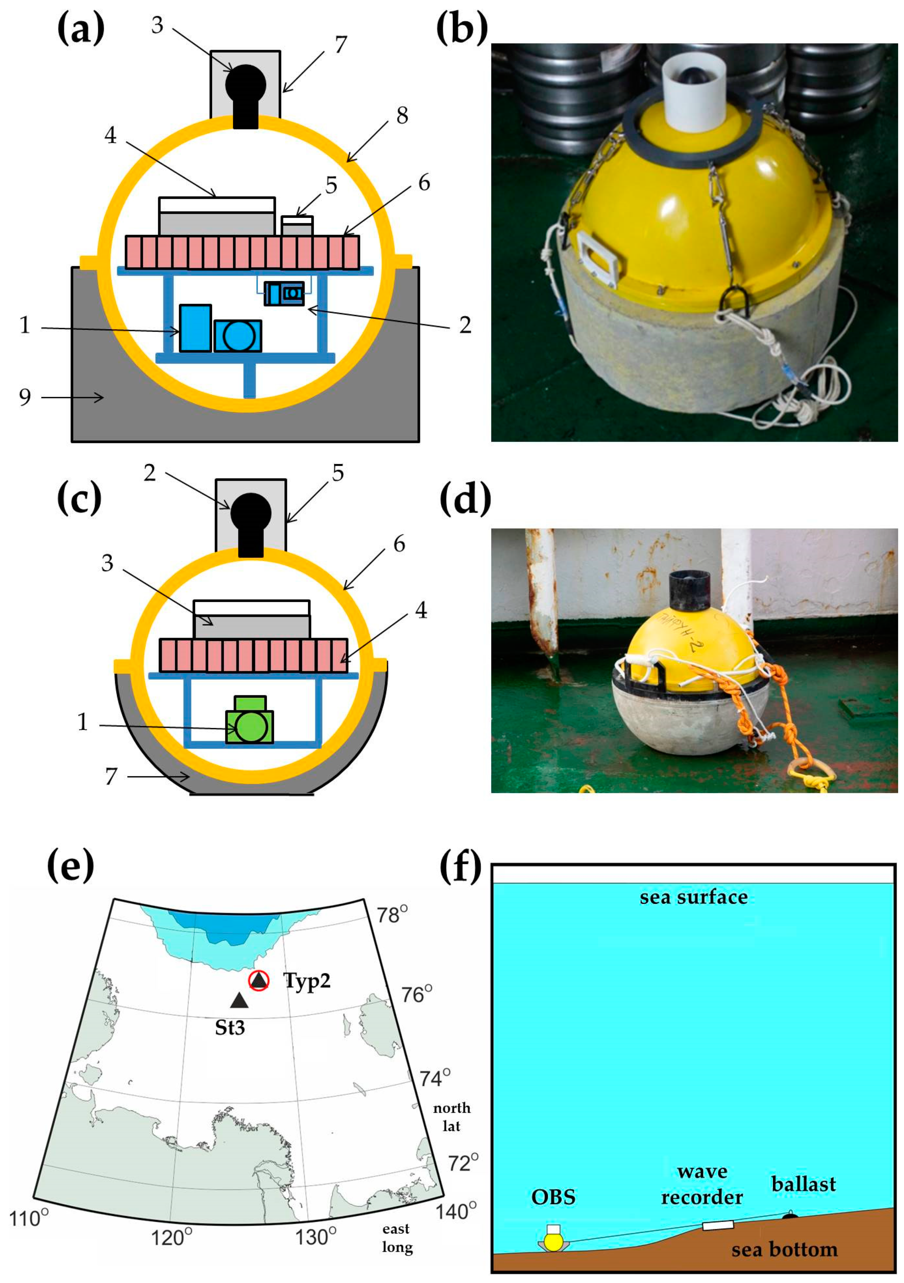
In this article, we have tried to develop an understanding of this method as applied to the marine environment. To achieve this objective, we used long-term OBS records obtained in the Laptev Sea, which is one of the most interesting regions from a seismotectonic point of view. This is especially true for the northern part of the Laptev Sea, the area of the outer shelf and the continental slope, where the Gakkel spreading ridge junctions with the shelf structures. In this area, many also assume the existence of a large strike-slip fault zone [7,8,9,10].

The presence of permafrost is widespread on the shelf of the Laptev Sea [11,12,13]. At the same time, in the central part of the outer shelf of the Laptev Sea, there is a zone of sparse permafrost and open taliks, which is confirmed by both the modeling results [12] and the data from offshore geophysical surveys [14,15].

In the Laptev Sea, a large number of methane outflows from the seabed have been found, especially on the mentioned central part of the outer shelf [16,17,18]. Recent studies show a deep thermogenic origin of the escaping gas on the outer shelf of the Laptev Sea [19]. Methane of deep origin can come from great depths along faults and reach the seafloor through wide taliks.

Until now, the application of the HVSR technique for the determination of the thickness of unfrozen sediments above the submarine permafrost has been very limited [20,21]. Many questions regarding the application of this method in marine shelf conditions, especially in the Arctic, and in particular in the presence of sea ice cover, remain open. Thus, the objective of the paper is to describe the features of applying the HVSR modeling and inversion techniques to seismic records obtained by OBSs on the outer shelf of the Laptev Sea, and to estimate the depth of the main shear wave impedance contrast, which can be associated with the transition from ice-free sediments to ice-bonded permafrost. In this case, the primary task is to describe the features of the recorded ambient seismic noise, which must be taken into account during HVSR modeling and interpretation. The processing of the ambient seismic noise recorded in the Laptev Sea, as well as the wave recorder data and the ERA5 and EUMETSAT reanalysis data, allowed the study of the dependency of seafloor seismic noise on the presence of sea ice cover, as well as sea waves in various frequency bands and weather conditions, wind speed in particular.

2. Data

2.1. OBS Data

Since 2018, a series of scientific cruises to the Laptev Sea and East Siberian Sea have been organized by the V.I. Ilichov Pacific Oceanological Institute of the Far Eastern Branch of the Russian Academy of Sciences and the Shirshov Institute of Oceanology of the Russian Academy of Sciences with the participation of a number of other institutions. The seismological research program has aimed to obtain the seismic and seismotectonic characteristics of the Laptev Sea region in the context of the relationship of the tectonic processes with the geohazards, the discharge of bubble methane from the bottom and the state of the submarine permafrost by registering local microearthquakes, remote teleseismic events and ambient seismic noise on the shelf and the continental slope of the Laptev Sea [22,23,24,25].

During the AMK-78 cruise (September–October 2019), two OBSs were deployed on the outer shelf of the Laptev Sea on board the R/V Akademik Mstislav Keldysh (Figure 1,

Table 1. The coordinates, types and dates of operation for the OBSs on the outer shelf of the Laptev Sea in 2019–2020 (for the station locations, see Figure 1e).

Site	Type	Latitude	Longitude	Depth	Operation Period
St3	MPSSR	76.392° N	125.660° E	51 m	9 October 2019–5 January 2020
Typ2	Typhoon	76.834° N	127.688° E	61 m	10 October 2019–9 February 2020

). They were dismantled in one year during the AMK-82 cruise (October 2020) on board the same vessel.

The two deployed OBSs were equipped with the three-component molecular–electronic transfer (MET) sensors: CME-4311 type in the MPSSR station at the St3 site, and CME-3311 type in the Typhoon station at the Typ2 site (Figure 1). The detailed parameters of the MET sensors are listed in

Table 2. Main technical parameters of the CME-4311 seismometer.

Frequency band *	0.0167 Hz (60 s)–50 Hz
Sensitivity	2000 V/(m/s)
Dynamic range at 1 Hz	123.5 dB
Power supply voltage	12 V (9.5–16 V acceptable)
Current consumption	8.5 mA
Temperature range	−12…+55 °C
Maximum inclination during installation	±15°

* indicated frequency range corresponds to the flat part of the response curve.

and

Table 3. Main technical parameters of the CME-3311 seismometer.

Frequency band *	1–50 Hz
Sensitivity	2000 V/(m/s)
Dynamic range at 1 Hz	118 dB
Power supply voltage	12 V (10.5–16 V acceptable)
Current consumption	25 mA
Temperature range	−12…+55 °C
Maximum inclination during installation	±15°

* indicated frequency range corresponds to the flat part of the response curve.

.

The OBSs also contained the hydrophone 5007 m and the URS-S recorder. The recorder URS-S can be used wherever multi-channel acquisition of analog signals with a reference to absolute time is required, with low power consumption.

Table 4. Main characteristics of the URS-S recorder.

Number of analog channels	4 (basic), 8 (extended)
Number of digital channels	1 (for reference to absolute time)
Sample rates	20, 25, 40, 50, 80, 100, 160, 200, 400, 800
Time synchronization	GPS interface
Temperature stability of the quarts generator	±5 × 10−9
Dynamic range	85–90 dB
Memory	SD card up to 64 Gb
Power supply voltage	6.5–32 V
Power consumption	20 mA (12 V)

shows the main characteristics of the URS-S recorder. The features of the recorder include its relatively low power consumption and the presence of a built-in high-precision thermo-stated reference frequency generator, in combination with a GPS interface, which makes it possible to time-tie the received records to absolute time.

The records duration was around 3 months for the MPSSR station and 4 months for the Typhoon station, while the recording frequency was 100 Hz. These types of OBS are not self-pop-up, and their housing is rigidly attached to the concrete ballast to improve traction on the seabed. The deployment in shallow waters was conducted with the use of the 150 m-long rope laid on the seabed and the ballast, according to the deployment scheme presented in Figure 1f. The deployment scheme implies trawling the rope between the OBS and the ballast. Thus, the current equipment and the deployment scheme imply work on the shelf at depths of no more than 100 m.

2.2. Wave Recorder Data

The Typhoon OBS at the Typ2 site was accompanied by the RBR virtuoso³ wave recorder (Figure 1). The records duration was 363 days, while the recording frequency was 1 Hz.

The RBR virtuoso³ logger is equipped with a Keller pressure sensor, based on the use of a piezoelectric quartz sensor, as a barosensitive element. It records the pressure values of the column of water and translates them into the variable depth of the location. The detailed parameters of the logger are listed in

Table 5. Main characteristics of the RBR virtuoso³ wave recorder (single channel logger).

Pressure range	100 m (dBar)–maximum accuracy
Initial accuracy	±0.05% FS (full scale)
Resolution	<0.001% FS
Typical stability	0.05% FS
Depth rating	750 m
Storage	240 M readings
Clock drift	±60 s/year
Power	8 AA cells

.

2.3. Reanalyses Data

The atmospheric parameters (hourly data), i.e., the mean sea level pressure and the northward and eastward component of the wind at 10 m above sea level, obtained from the ERA5 reanalysis [26] were used in the research. Daily ice concentration data were provided by EUMETSAT [27]. Horizontal resolution of the reanalysis for atmospheric parameters was 0.25° for ice concentration–25 km.

To obtain the required parameters from the atmospheric reanalysis data for specific points in the Laptev Sea, the nearest points on the reanalysis grid were selected. Bilinear interpolation between the four nearest points was used for the ice concentration data. Further, for each reanalysis point, records were selected corresponding to the dates of measurements of seismological and sea-level sensors.

3. Methods

3.1. Raw Records Processing and Seismic Noise Spectrograms Calculation

First of all, the reading, conversion and pre-processing of the OBS seismic records are performed. After reading from the flash memory of the seismic recorder, the raw records are contained in files of specific binary format with the samples of five channels: a hydrophone, three components of a velocimeter, and a channel of accurate time samples. Next, the raw binary files are batch converted into one of the generally accepted seismological formats, miniSEED, using Matlab scripts and some Seisan conversion utilities [28]. After that, the records are ready for seismological analysis.

By using seismic noise spectrograms, we assessed the temporal variability of observations in order to distinguish the effects of ice cover, wind-generated gravity waves, infragravity waves, and atmospheric parameters, such as atmospheric pressure and wind speed. Spectrograms of the seismic records were calculated with standard functions of the Matlab environment, which implement short-time Fourier transform [29,30,31,32] with the use of a sliding Hamming window and 50% overlap between segments. The records were preliminary averaged in 1-s long windows. Calculations on long time series from different source files were performed sequentially with subsequent concatenation of the resulting array. A spectrogram of the sea level records in the range of periods from 30 to 300 s was calculated with Welch’s method [33], using the Kaiser–Bessel spectral window two days long, with 50% overlap.

3.2. HVSR Modeling

The average HVSR curves were computed by Geopsy software (http://www.geopsy.org, accessed on 15 September 2022) [34] following standards from the SESAME project manual [35].

Table 6. The input parameters for the HVSR modeling.

Parameter	Value (for St3 Records)	Value (for Typ2 Records)
Record duration	~6 h	~8 h
Window length	25 s.	25 s.
Filtering	no	no
STA	1 s.	1 s.
LTA	30 s.	30 s.
Min STA/LTA	0.2	0.2
Max STA/LTA	2.5 (Oct); 2.5 (Nov); 3.9 (Dec)	1.83 (Oct); 1.35 (Nov); 1.24 (Dec)
Number of windows	24 (Oct); 29 (Nov); 26 (Dec)	27 (Oct); 27 (Nov); 28 (Dec)
Horizontal components	squared average	squared average
Taper window type	Tukey, width 5%	Tukey, width 5%
Smoothing	rectangular window, width 1 Hz	rectangular window, width 1 Hz

shows the input parameters for the HVSR calculations separately for St3 site records and for Typ2 site records. The input parameters were chosen so that the number of windows and samples in each window met the requirements from the SESAME guideline for the expected fundamental frequency.

At the first stage, a set of 25-s long time windows was selected by the STA/LTA “antitrigger” algorithm, based on [35,36,37], so that the STA/LTA values were between the specified maximum value to avoid transients and minimum values, to avoid anomalously low amplitudes. No preliminary filtering was applied. No overlapping was applied since the total duration of the noise record was enough.

HVSR computations were conducted as follows for each time window with the following averaging of the resulting curves:

$$\mathit{HVSR}=\frac{\sqrt{({\left|H_1\right|}^2+{\left|H_2\right|}^2)/2}}{\left|V\right|}$$

(1)

where H₁ and H₂ are Fourier spectra amplitudes of the two horizontal components of seismic noise, while V is the Fourier spectrum amplitude of the vertical component of seismic noise.

Since the raw spectra contain a lot of frequency samples which show a lot of very narrow oscillations and spikes, while computing the HVSR, the very small values reached by raw spectra lead to unusual values of the ratio. Therefore, before computing the HVSR, the Fourier spectra amplitude of the three components were smoothed by a rectangular window of 1 Hz width.

3.3. HVSR Inversion

We considered a one-dimensional two-layer soil system with a dominant and sharp acoustic impedance contrast below a shallow surface layer at depth d. Let the frequency f₀ be the main peak in the HVSR curve, i.e., the lowest dominant peak frequency. The f₀ can be associated to the fundamental seismic resonance frequency f_reson related to the interference of transmitted and reflected from the interface of impedance contrast waves. The seismic resonance frequency of the n-th mode is related to the shear velocity v_s and thickness of the overlying layer d as follows [21]:

$$f_{\mathit{reson}}=(2n+1)\frac{v_s}{4d}$$

(2)

where frequency is given in Hz, shear waves velocity in m/s, and layer thickness in m.

If we know the value of the shear wave velocity from the results of the field work or from reference materials, and the value of the resonant frequency from the HVSR curves, then we can easily estimate the depth of the contrast boundary using the Formula (2). The value of shear wave velocity, density of the surface layer soil and the underlying half-space, as well as the thickness of the surface layer estimated using Formula (2), can be used to construct the subsurface soil model, which in turn, along with HVSR curves, can serve as initial data for optimization by inversion methods.

In this paper, HVSR inversion was conducted by OpenHVSR software [38]. The inversion strategy is based on the Monte Carlo method, where at every iteration a randomly perturbed version of the best-fitting model is produced and used to compute a set of simulated curves to be compared with the experimental HVSR curves. The forward simulation of the theoretical transfer function curves is based on the approach of [39]. A criterion to decide which simulated curve best reproduces the experimental data is based on calculating the value of an objective function, which is a positive, real-value function of the subsurface parameters, and the misfit between the data and the simulated curves, and seeking its global minimum.

4. Results

4.1. Correlation of the Reanalysis, Wave Recorder and OBS Data

Figure 2 shows a comparison of the time dependences of the atmospheric parameters obtained from the reanalysis data, the sea level fluctuations in the frequency band 0.05–0.5 Hz [40], related to the wind-generated gravity sea waves obtained from the wave recorder data, as well as the ground velocity fluctuations obtained from the Typ2 OBS hydrophone and seismometer records. Since the reanalysis data are hourly, the averaging of the wave recorder and seismometer data was also carried out in hourly windows. The curves corresponding to the seismometers’ data were also additionally smoothed in a moving average window (30,000 points).

The semi-transparent colored numbered rectangles indicate the specific time periods, characterized by a certain pattern. The blue rectangle 1 corresponds to the period of time when the sea was free of ice—this can be seen from the ice concentration curve. During this period of time, the wave recorder, hydrophone and seismometers data curves correlated well with the wind speed curves. The peak positions of the curves are in good agreement with each other. The red rectangle 2 corresponds to the period of time of rapid ice formation, and also a sharp decrease in the amplitudes of sea level fluctuations and the level of seismic noise on all seismic sensors. The yellow rectangles 3–5 indicate the time intervals of a remarkable and rather long increase in the amplitudes of sea level fluctuations and seismic noise level within the period when the sea was covered with ice. These time intervals coincide with the moments of short but sharp wind speed increase above 14 m/s and also with a short but sharp drop in atmospheric pressure.

Figure 3 shows the spectrograms of the ambient seismic noise obtained from the records of the OBS seismometers at the St3 and Typ2 sites. Colored arrows indicate the notable spectrogram features. First, the spectrograms also clearly show the differences between the period of time when the sea was ice-free and the period when the sea was covered with ice. The absence of ice is reflected in a pronounced signal amplification in the low-frequency ranges of 0.1–0.2 Hz and 0.3–1.5 Hz. On the spectrograms corresponding to the St3 site, the signal amplification in the frequency range 0.1–0.2 Hz is more pronounced than in the range 0.3–1.5 Hz, while on the spectrograms corresponding to the Typ2 site, the opposite is true. This is explained by the fact that the CME-4311 seismometers at the St3 site are broadband, and the CME-3311 sensors at the Typ2 site are short-period with a fundamental frequency of 1 Hz. Due to the fact that the sensitivity of the CME-3311 sensor at frequencies below 1 Hz does not decrease immediately, signal amplification is still present down to 0.1 Hz. The yellow arrows indicate the boundary between ice-free and ice-covered time periods.

The remarkable increases in the amplitudes of seismic noise level within the period when the sea was covered with ice, highlighted in Figure 2 as yellow rectangles 3–5, are also visible on the spectrograms in Figure 3 (see the red arrows). In addition, the spectrogram shows a time-constant signal amplification in a narrow frequency band in the vicinity of 10 Hz (indicated by the white arrows), and in some time periods also in narrow frequency bands in the vicinity of 18 and 30 Hz (indicated by the orange arrows). In the time period after 9 December, the same constant signal amplifications appear in narrow frequency bands in the vicinity of 8 and 15 Hz (indicated by the gray arrows).

Figure 4 shows on a larger scale the time history of wind speed at the Typ2 site and its correlation with the increase of the seismic noise level shown on the spectrogram obtained for the horizontal seismometer at the Typ2 site. It can be seen that the signal amplification at 10 Hz is present all the time at any wind strength (indicated by the white arrows), while with an increase in wind speed this signal becomes more pronounced. In this case, additional maxima appear at 18 and 30 Hz (indicated by the orange arrows).

Figure 5 demonstrates the correlation between sea level fluctuation in the 30 s–5 min spectral periods range (related to infragravity sea waves [40]) obtained by the wave recorder RBR virtuoso³ and its spectrogram, the horizontal component of ground velocity, obtained by the OBS at the Typ2 site, and the wind speed. The green rectangle 1 corresponds to the period of time when the sea was ice-covered and seismic noise levels were low. At the same time, there was a low level of infragravity waves amplitudes and wind speed. In the time period after 8 December, indicated by the purple rectangle 2, there was ice either, and short but very frequent peaks in the level of seismic noise were observed, as well as an increase in the level of amplitudes of infragravity waves and wind speed. The energy level of infragravity waves and wind speeds fluctuate almost identically.

4.2. HVSR Modeling Results

Figure 6 shows the HVSR time-frequency plots for the OBS records obtained at the St3 and Typ2 sites. The pink arrows indicate the parts of the spectrograms that are characterized by a reduced level of HVSR in the low-frequency band of 0.2–2 Hz, which makes the high-frequency peaks above 2 Hz more pronounced than in the parts of the spectrograms indicated by the black arrows.

The low level of HVSR in the low-frequency band of 0.2–2 Hz is observed during the period of time when the sea was free of ice. When there is ice on the sea, the signal level becomes flatter over the entire time and frequency range. However, a clear HVSR maximum at 10 Hz is observed throughout the entire observation period (indicated by the white arrows). At the same time, a less pronounced constant HVSR maximum at 3 Hz is observed only in the spectrogram corresponding to the St3 site (indicated by the red arrow). The spectrogram corresponding to the Typ2 site has weak permanent maxima at 8 and 15 Hz that appear after December 8 (indicated by the gray arrows). The parts of the spectrograms below 0.2 Hz for the St3 site and below 0.6 Hz for the Typ2 site are not representative.

Figure 7 and Figure 8 show the examples of the time window selection for HVSR modeling and the results of the HVSR modeling, correspondingly. For the HVSR modeling, we selected 6–8 h long OBS records obtained at the St3 and Typ2 sites on 25 October, 25 November and 25 December 2019. The time periods were chosen in such a way as to obtain separate results for three different months, because they are characterized by different weather and ice conditions.

In Figure 8, two characteristic frequency ranges are distinguished on the HVSR curves for the St3 site: 2–5 Hz with a maximum at 3 Hz (pink rectangle 1) and 6–15 Hz (gray rectangle 2) with a maximum at 9–10 Hz. On the HVSR curves for the Typ2 site, there is only one high-frequency characteristic frequency range 5–15 Hz with a maximum at 9–10 Hz.

The maximum of the curves at 9–10 Hz is most likely due to the coupling effect, a distortion of high frequencies of records due to parasitic oscillations in the system “station–ballast–soft sediments” [41], which is usually observed in the high-frequency range of 5–10 Hz. This issue will be covered in more detail in the Discussion section.

Therefore, the resonant peak associated with the presence of a contrast reflective boundary under the seabed surface can be considered at a maximum of 3 Hz for the St3 site, which is more pronounced for the time period with an ice-free sea. Accordingly, there is no such resonance peak at all in the considered frequency range for the Typ2 site.

4.3. HVSR Inversion Results

Table 7. The initial subsurface model for HVSR inversion for the St3 site.

Vp (P-Waves Velocity) [m/s]	Vs (S-Waves Velocity) [m/s]	Rho (Density) [g/cm3]	d (Thickness) [m]	Qp (P-Waves Damping) [%]	Qs (S-Waves Damping) [%]
430	210	1.8	18	15	5
2600	1100	1.8	half-space

and

Table 8. The initial subsurface model for HVSR inversion for the Typ2 site.

Vp (P-Waves Velocity) [m/s]	Vs (S-Waves Velocity) [m/s]	Rho (Density) [g/cm3]	d (Thickness) [m]	Qp (P-Waves Damping) [%]	Qs (S-Waves Damping) [%]
430	210	1.8	70	15	5
2600	1100	1.8	half-space

show the parameters of the subsurface soil model for the St3 and Typ2 sites correspondingly, which, along with the HVSR curves, were used as initial data for inversion. It is known that the shelf area where the OBSs were deployed is characterized by silty surface soils [42]. In addition, based on the characteristics of the region, we assume that the sub-bottom reflecting boundary was most likely the upper surface of the permafrost. In accordance with this, the values of the P- and S-waves velocity, as well as the density of the soil, were selected from reference materials [43]. The thickness of the surface layer (18 m) for the St3 site was estimated using Formula (2). Since it can be seen from Figure 8 that at the Typ2 site there is no resonant peak related to the contrast sub-bottom boundary, we assumed that its depth was beyond the values corresponding to representative seismic sensor frequency band, i.e., lower than 1 Hz. Therefore, according to Formula (2), we determined that for the Typ2 site, the depth of the reflecting boundary should be more than 53 m, so the value of 70 m was taken.

Figure 9 shows the schematic view of the OBSs deployed in the Laptev Sea with indication of sea depths and representation of the resonance effect and its relation to soil amplification curves. Figure 10 shows, in turn, the assumed initial velocity profiles for the St3 and Typ2 sites.

Figure 11 shows the results of the HVSR inversion. In general, a correspondence was obtained between the simulated curves and the curves obtained from the observational data, i.e., the amplitude and position of the resonance peak for the St3 site, as well as the position and shape of the curves for the Typ2 site.

Table 9. The optimized subsurface model obtained by HVSR inversion for the St3 site.

Vp (P-Waves Velocity) [m/s]	Vs (S-Waves Velocity) [m/s]	Rho (Density) [g/cm3]	d (Thickness) [m]	Qp (P-Waves Damping) [%]	Qs (S-Waves Damping) [%]
512	279	1.8	17.7	15	5
2600	1100	1.8	half-space

and

Table 10. The optimized subsurface model obtained by HVSR inversion for the Typ2 site.

Vp (P-Waves Velocity) [m/s]	Vs (S-Waves Velocity) [m/s]	Rho (Density) [g/cm3]	d (Thickness) [m]	Qp (P-Waves Damping) [%]	Qs (S-Waves Damping) [%]
1833	611	1.8	329	15	5
2600	1100	1.8	half-space

show the optimized subsurface models obtained by HVSR inversion for the St3 and Typ2 sites, while Figure 12 shows the optimized velocity profiles.

5. Discussion

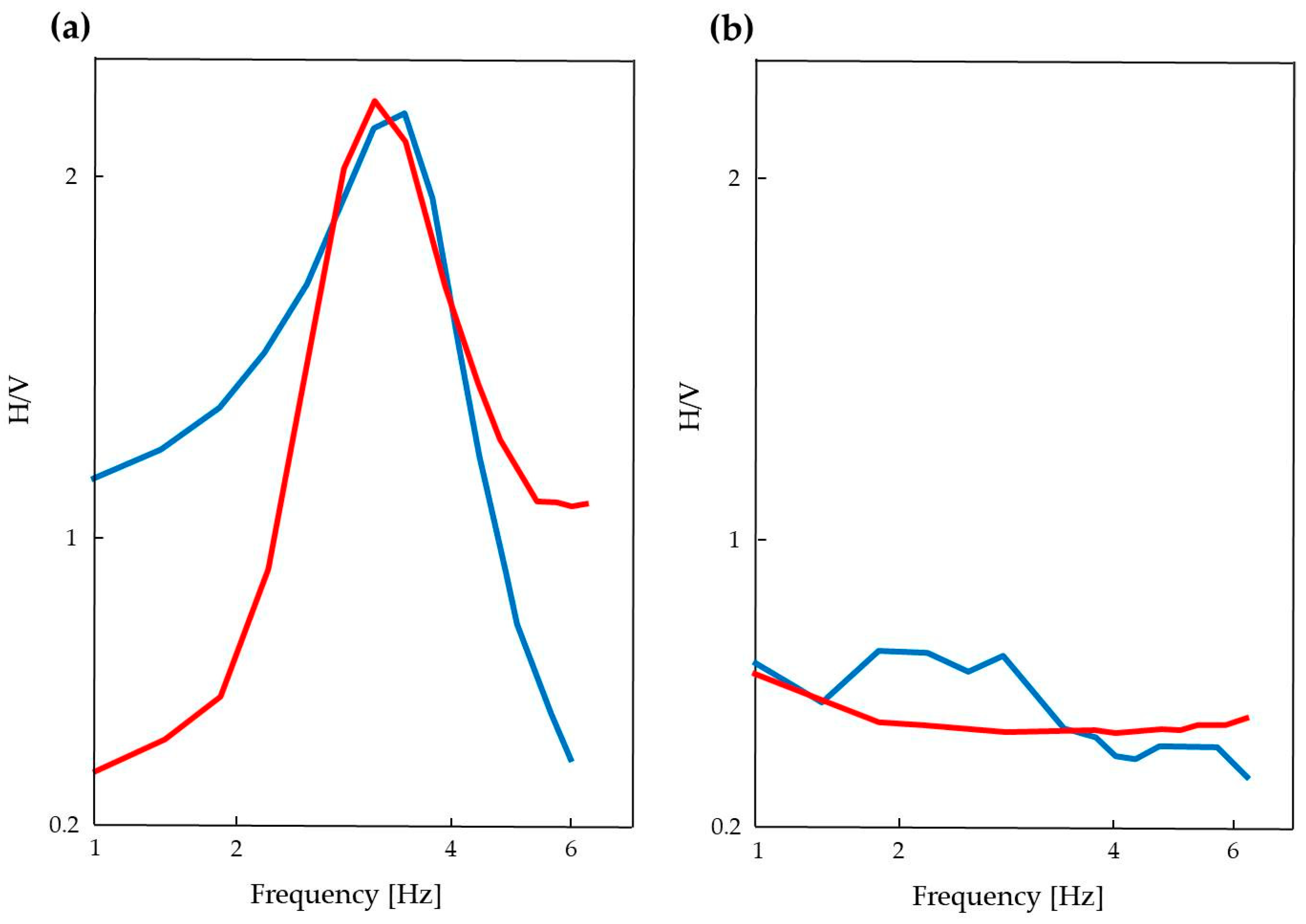
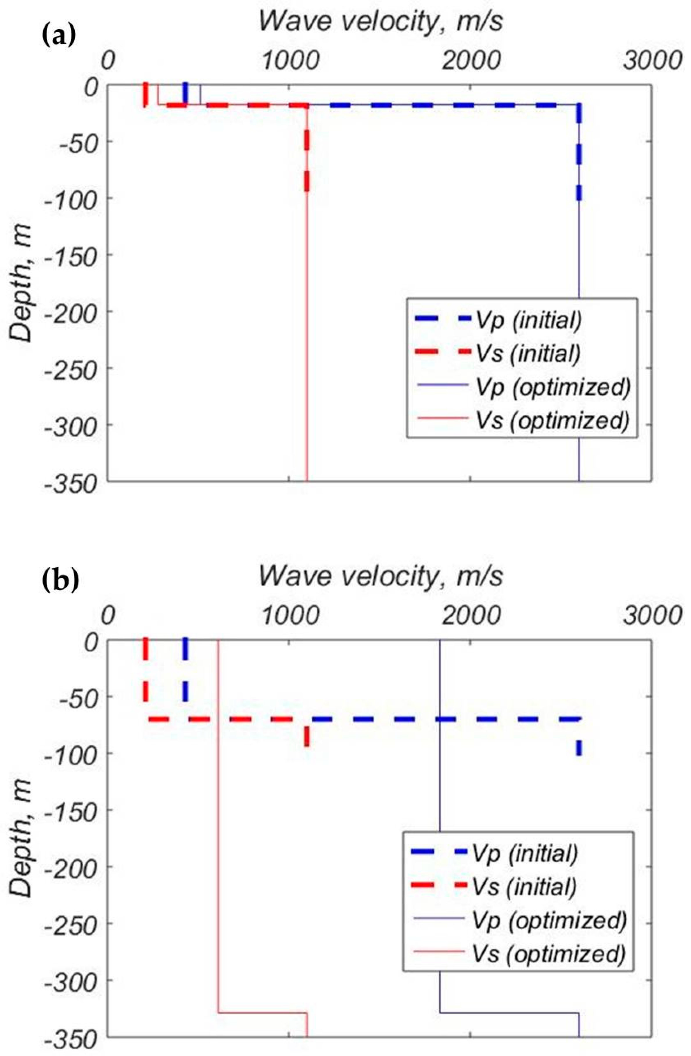
A description of seafloor seismic noise features is necessary for HVSR modeling and interpretation. Only by taking into account the characteristics of seismic noise is it possible to adequately select a frequency confidence range for further searching for resonant peaks associated with a contrasting reflective boundary under the seabed surface. In the present study, such a confidence frequency range was between 1 and 6 Hz. 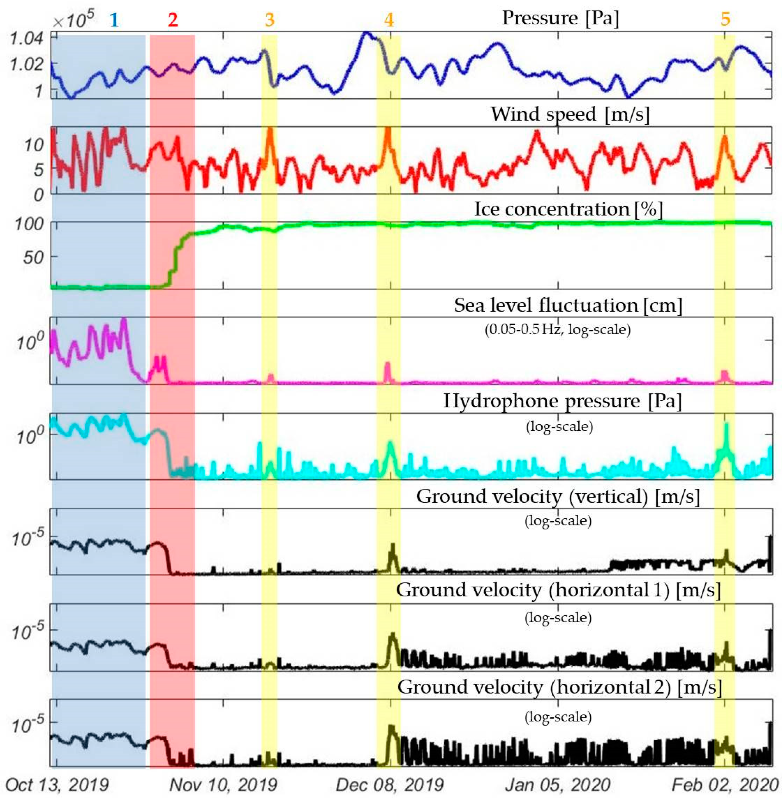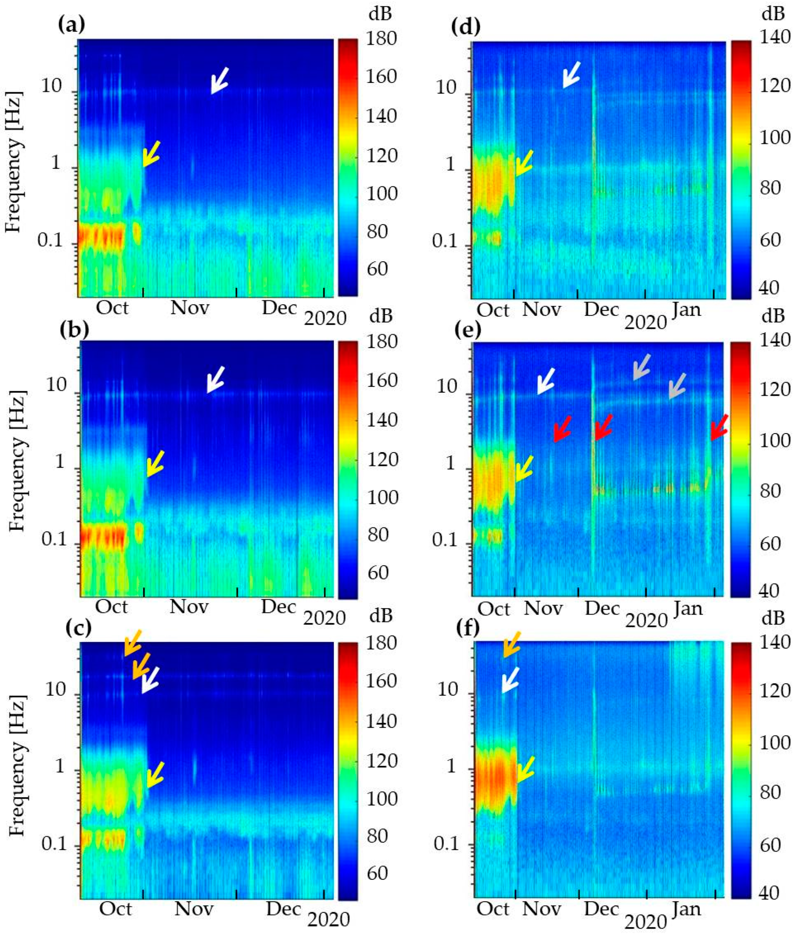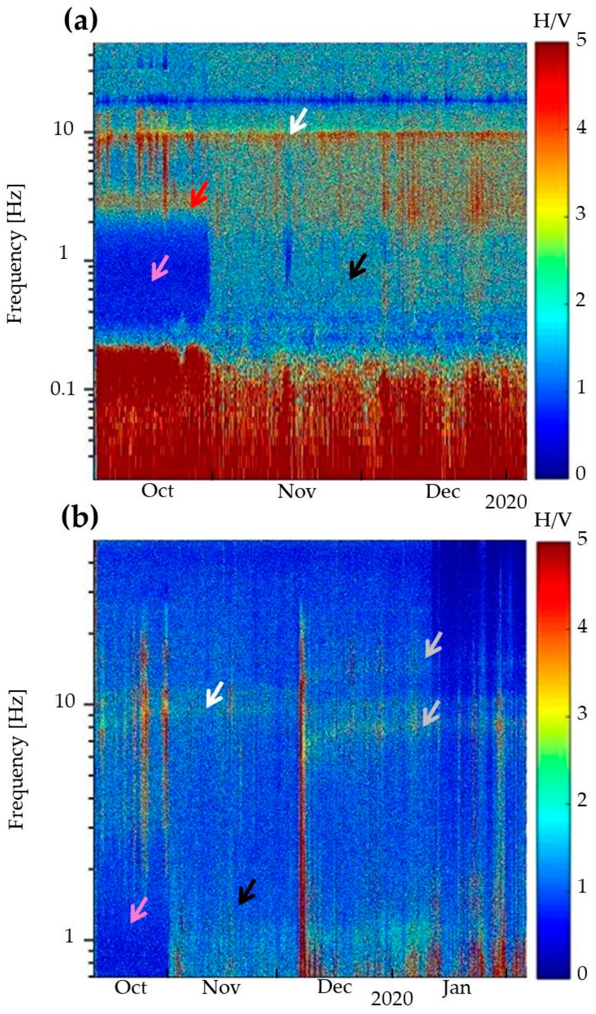It was this frequency range that was used for the HVSR inversion (Figure 11). The level of seismic noise at frequencies below 1 Hz at the studied shelf sites strongly depended on the intensity of the wind waves of the sea, and therefore on the wind speed and the presence of ice cover. The maximum level of seismic noise during the period of time when the sea was ice-free was in the frequency ranges 0.1–0.2 Hz and 0.3–1.5 Hz (Figure 2 and Figure 3), related to primary and secondary microseisms, which are recorded everywhere and are the result of processes related to sea gravity waves and atmospheric pressure [41,44,45]. When the sea was covered with ice, this low-frequency seismic noise level decreased, but nevertheless remained, periodically increasing at certain intervals under the influence of an increase in wind speed and a drop in atmospheric pressure (Figure 2 and Figure 3). The wind effect on seismic noise has also been noticed for on-land seismographs. It is present in the low frequency range and is caused by natural wind directly blowing on the sensor [46,47,48,49].

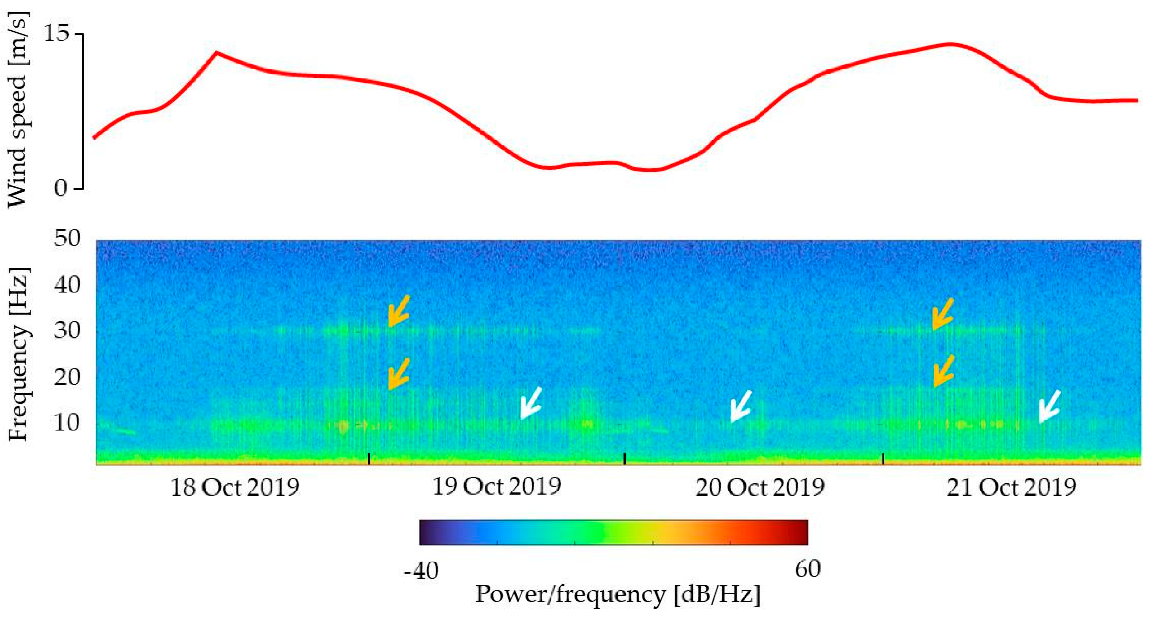
The high-frequency seismic noise at frequencies above 6 Hz with the clear maximum at 9–10 Hz is highly distorted by the parasitic oscillations in the system “station–ballast–soft sediments” (coupling effect), which is usually observed in the high-frequency range of 5–10 Hz [41]. While the signal amplification at 10 Hz was present all the time at any wind strength, the additional parasitic oscillations maxima appear at 18 and 30 Hz with an increase in wind speed (Figure 4).

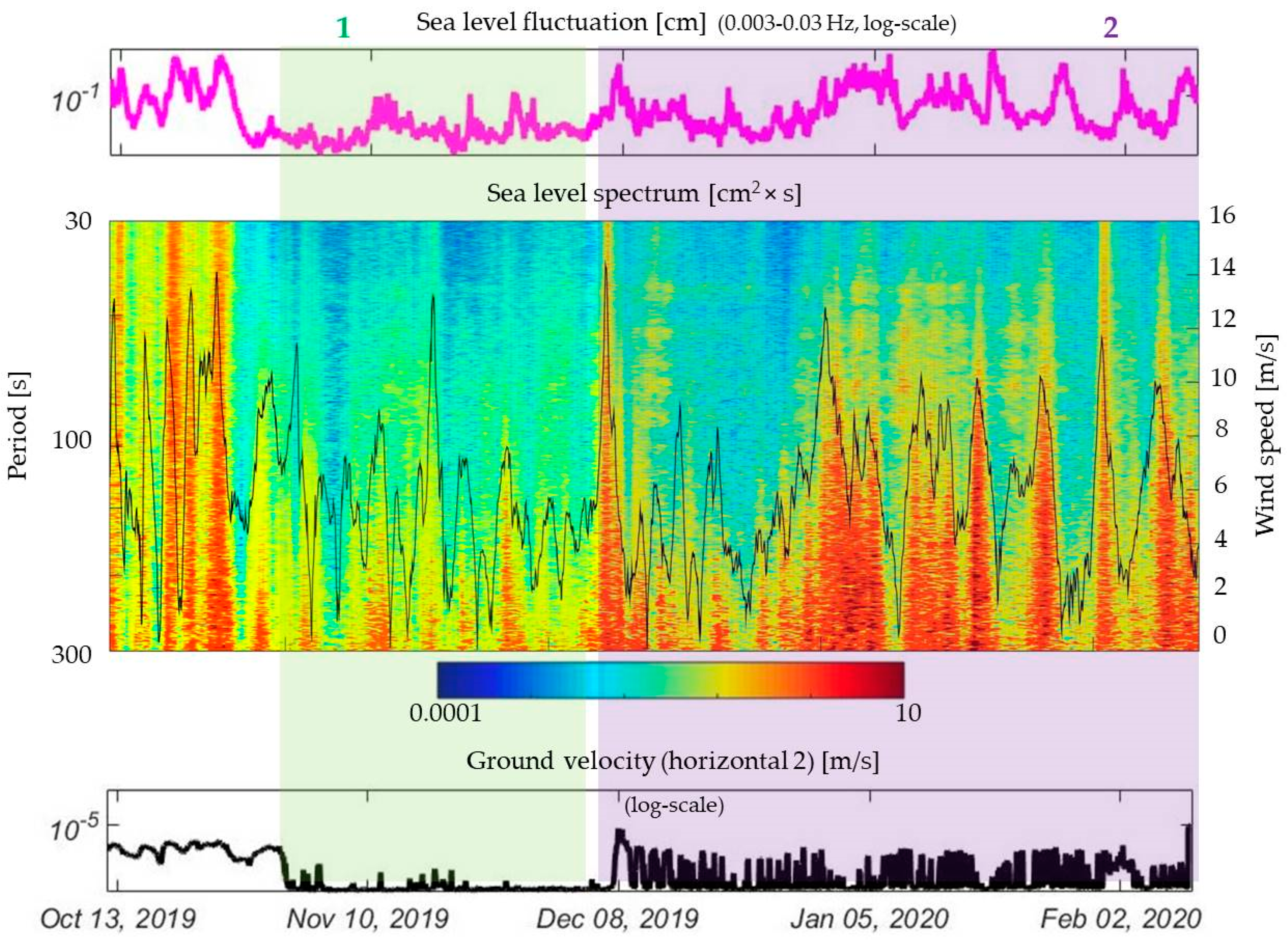
There is a clear correlation between sea level fluctuation in the 30 s–5 min spectral periods range related to infragravity sea waves [40,50,51], ambient seismic noise and wind speed, as seen in Figure 5. This pattern may be due to the supposed similarity of the mechanisms behind the generation of the ocean infragravity waves and seismic noise [51]. Long-period horizontal noise levels for sensors on the seafloor are higher than vertical noise levels [41], as also seen in Figure 2. Interestingly, sea level fluctuations in the spectral range related to infragravity waves correspond to fluctuations in wind speed better than ordinary gravity waves. Perhaps this is due to the fact that the infragravity waves have a larger length and are more stable in time. The ordinary wind-generated gravity waves and swell are less stable, since they have a shorter period (5–8 s), while the infragravity waves are more inert. This is important, especially since the reanalysis data was measured hourly. Separately, it is necessary to note the excellent agreement between the reanalysis data and the observational data.

Long-period seismic noise with spectral periods larger than 30 s is associated with both infragravity waves and seafloor currents [41]. Current-induced tilt noise is caused by seafloor currents flowing past the instrument and in eddies spun off the back of the instrument [52,53,54]. The current noise at deep seafloor sites is usually orders of magnitude larger than infragravity wave noise [41], but at shallow depths this could be the reverse, especially in view of the fact that, according to the data obtained, no obvious dependence of seismic noise on tides was revealed, i.e., characteristic periodicity, while Figure 5 demonstrates significant correlation between the amplitudes of infragravity waves and seafloor seismic noise. Thus, it can be assumed that at the considered sites, the effect of infragravity waves on long-period seismic noise is predominant.

Even though infragravity wave amplitudes decrease with increasing ocean depth, the signal remains significant to depths of many kilometers below the seabed depending on the frequency and the elastic parameters as a function of depth [41]. At shallow depths, gravity and infragravity waves can drive motions directly, tilting the instrument [41,55,56]. However, it is difficult to estimate the relative contribution of the direct tilting of the instrument to the total level of recorded long-period noise.

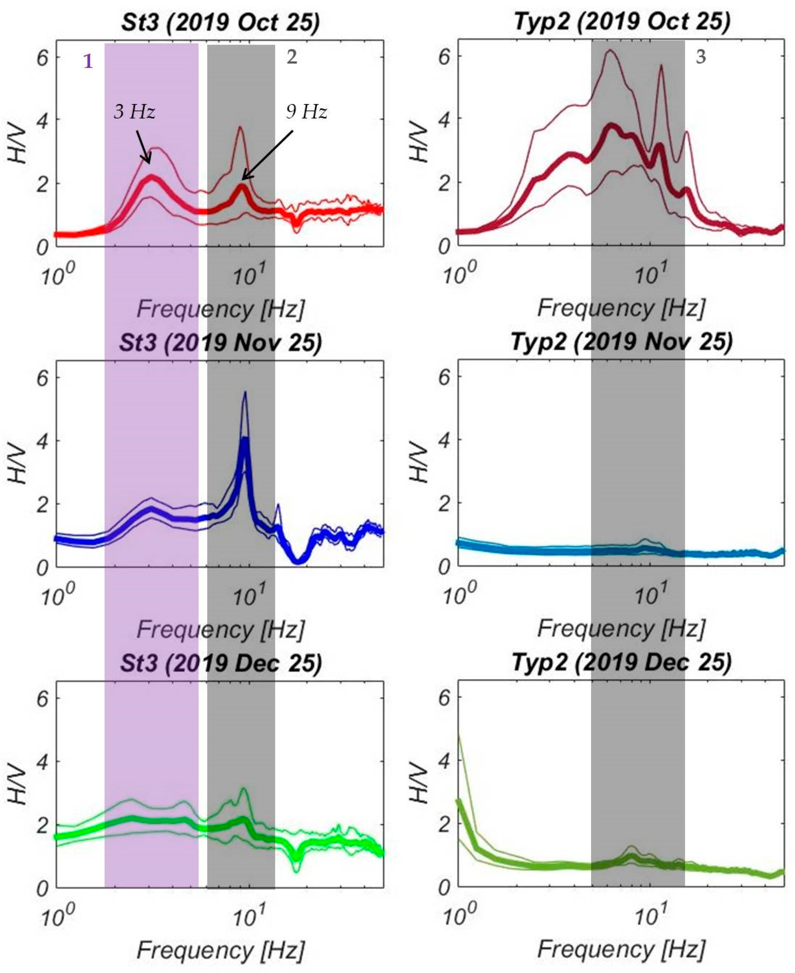
The HVSR time-frequency plots presented in Figure 6 show the reduced level of HVSR in the low-frequency band of 0.2–2 Hz during the period of time when the sea was free of ice. This makes the high-frequency peaks above 2 Hz more pronounced. This can be explained by the fact that an increased level of seismic noise in the frequency range 0.2–2 Hz, caused by the wind waves of the sea, is observed both on the horizontal and vertical components of seismometers. Therefore, the ratios of the smoothed spectral curves have low values in this frequency range. In the same time period, when there was ice on the sea and the seismic noise caused by the wind waves was reduced, the HVSR curve becomes flatter over the entire time and frequency range. The signal maximum at 9 Hz, which corresponds to the coupling effect, is also well pronounced on the HVSR curves.

HVSR can also be used to estimate the ellipticity of the fundamental mode Rayleigh wave, which has the advantage of defining the total depth of the soft sediments [57]. The principal problem of retrieving ellipticity from HVSR spectral ratios is to correct for the energy of body and Love waves present in the ambient vibration recordings [58,59]. This could be provided by classical polarization analysis in the frequency domain or by identifying P-SV wavelets along the signal and computing the spectral ratio from these wavelets only [59]. In the framework of this work, these methods were not considered.

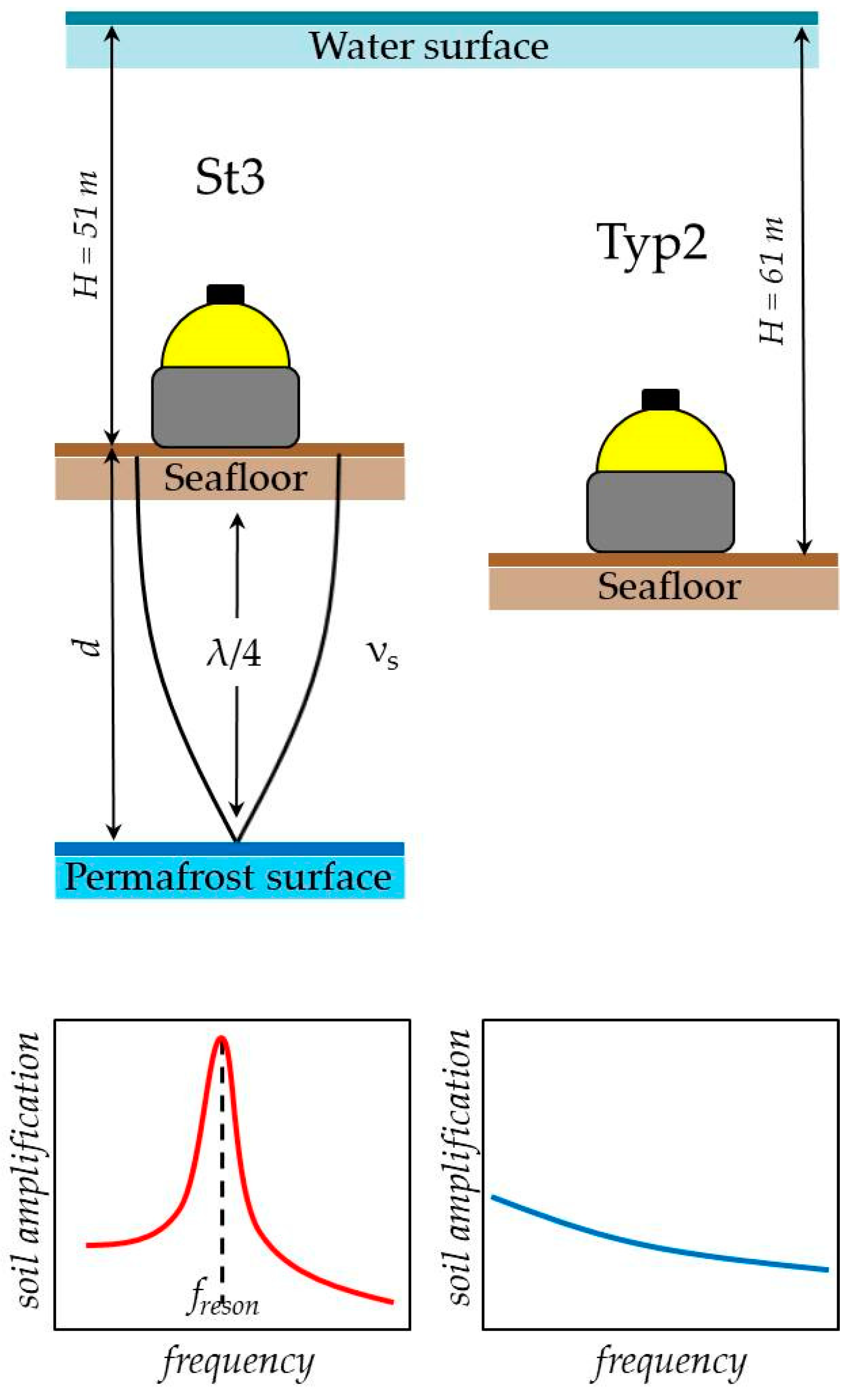
Based on the characteristics of the region where the OBSs were deployed, we assumed that the sub-bottom reflecting boundary, most likely, would be the upper surface of the permafrost, and the layer of soft sediments above it would consist of silty soils. Since the exact values of soil densities and seismic wave velocities for the study area are unknown, their values were taken from reference materials. All this together leads to a significant uncertainty in the assessment of the depth of the reflecting boundary and the results of the HVSR inversion. In the case of the Typ2 site, the inversion is further complicated by the absence of a resonant peak in a representative frequency range of the HVSR curve. Therefore, the results of the inversion for the Type2 site should be treated as very approximate. It should also be noted that due to the fact that the inversion is based on the Monte Carlo method, the result obtained can be considered as only one of the possible solutions.

Many papers present formulas that correlate cover thickness with the frequency of the HVSR main peak [49,60,61,62,63,64]. All of them have the following general form:

$$d=a{f}_{\mathit{reson}}^b$$

(3)

Table 11. Different estimates of the thickness of soft sedimentary cover above the assumed permafrost layer at the St3 site.

Source	a	b	d [m]
Ibs-von Seht and Wohlenberg, 1999 [60]	96	−1.388	20.9
Parolai et al., 2002 [61]	108	−1.551	19.7
Guo et al., 2014 [49]	24.87	−0.6852	11.7
Abd et-aal, 2018 [62]	90	−1.45	18.3
Moon et al., 2019 [63]	92.5	−1.06	28.9
Guo et al., 2021 [64]	116.7	−1.367	25.9

shows the values of the parameters a and b obtained from different sources, along with corresponding values of calculated d for the St3 site. It can be seen that the thickness values vary significantly from 11.7 to 28.9 m, which is quite understandable, because these empirical formulas were obtained in different regions and for different parameters of soils. In the present study, a thickness value of 17.7 m was obtained. The formulas from [61,62] give the closest estimate.

6. Conclusions

(1)

The results of processing of the recorded ambient seismic noise, as well as the wave recorder data and ERA5 and EUMETSAT reanalysis data, showed a strong dependence of seafloor seismic noise on the presence of sea ice cover, as well as weather conditions, wind speed in particular. Wind-generated gravity waves, as well as infragravity waves, are responsible for the increase in the level of ambient seismic noise. The high-frequency range of 5 Hz and above is strongly affected by the coupling effect, which in turn also depends on wind-generated gravity waves and infragravity waves. The described seafloor seismic noise features must be taken into account during HVSR modeling and interpretation.

(2)

The obtained HVSR curves plotted from the records of one of the OBSs revealed a resonant peak corresponding to 3 Hz, while the curves plotted from the records of another OBS did not show clear resonance peaks in the representative frequency range. Since both OBS were located in the area of sparse distribution of submarine permafrost, the presence of a resonance peak may be an indicator of the presence of a contrasting boundary of the permafrost upper surface under the location of the OBS. The estimation of the depth to permafrost boundary for the St3 site is around 18 m. The absence of a clear resonant peak in the HVSR curve for the Typ2 site may indicate that the permafrost boundary was either absent at this site or its depth was beyond the values corresponding to representative seismic sensor frequency band. Thus, HVSR modeling and inversion techniques can be effective for studying the position of submarine permafrost.

References

1. Kang, S.Y.; Kim, K.-H.; Chiu, J.-M.; Liu, L. Microtremor HVSR analysis of heterogeneous shallow sedimentary structures at Pohang, South Korea. J. Geophys. Eng. 2020, 17, 861–869. [Google Scholar] [CrossRef]
2. Xu, R.; Wang, L. The horizontal-to-vertical spectral ratio and its applications. EURASIP J. Adv. Signal Process. 2021, 2021, 75. [Google Scholar] [CrossRef]
3. Aleshin, I.M.; Goev, A.G.; Kosarev, G.L.; Presnov, D.A. Seismic Noise H/V Spectral Ratio Can Be Inverted Jointly with Receiver Functions. Izv. Phys. Solid Earth 2021, 57, 559–566. [Google Scholar] [CrossRef]
4. Kalinina, A.V.; Ammosov, S.M.; Tatevossian, R.E.; Turchkov, A.M. Using Microseisms for Seismic Microzoning. Seism. Instr. 2022, 58, 398–408. [Google Scholar] [CrossRef]
5. Nogoshi, M.; Igarashi, T. On the amplitude characteristics of microtremor (Part 2). J. Seism. Soc. Jpn. 1971, 24, 26–40, (In Japanese with English abstract). [Google Scholar]
6. Nakamura, Y. A method for dynamic characteristics estimations of subsurface using microtremors on the ground surface. Railw. Technol. Res. Inst. Quart. Rep. 1989, 30, 25–33. [Google Scholar]
7. Drachev, S.S. Laptev Sea Rifted Continental Margin: Modern Knowledge and Unsolved Questions. Polarforschung 2000, 68, 41–50. [Google Scholar]
8. Drachev, S.S.; Kaul, N.; Beliaev, V.N. Eurasia spreading basin to Laptev Shelf transition: Structural pattern and heat flow. Geophys. J. Int. 2003, 152, 688–698. [Google Scholar] [CrossRef]
9. Shipilov, E.V.; Lobkovsky, L.I.; Shkarubo, S.I. Structure of the Khatanga–Lomonosov Fracture Zone according to Seismic Data. Dokl. Earth Sci. 2019, 487, 846–851. [Google Scholar] [CrossRef]
10. Shipilov, E.V.; Lobkovsky, L.I.; Shkarubo, S.I. Khatanga-Lomonosov fault zone: Structure, tectonic position and geodynamics. Arct. Ecol. Econ. 2019, 3, 47–61. (In Russian) [Google Scholar] [CrossRef]
11. Romanovskii, N.N.; Hubberten, H.-W. Results of Permafrost Modelling of the Lowlands and Shelf of the Laptev Sea Region, Russia. Permafr. Periglac. Process. 2001, 12, 191–202. [Google Scholar] [CrossRef]
12. Nicolsky, D.J.; Romanovsky, V.E.; Romanovskii, N.N.; Kholodov, A.L.; Shakhova, N.E.; Semiletov, I.P. Modeling sub-sea permafrost in the East Siberian Arctic Shelf: The Laptev Sea region. J. Geophys. Res. 2012, 117, F03028. [Google Scholar] [CrossRef]
13. Matveeva, T.V.; Kaminsky, V.D.; Semenova, A.A.; Shchur, N.A. Factors Affecting the Formation and Evolution of Permafrost and Stability Zone of Gas Hydrates: Case Study of the Laptev Sea. Geosciences 2020, 10, 504. [Google Scholar] [CrossRef]
14. Bogoyavlensky, V.I.; Kishankov, A.V.; Kazanin, A.G. Permafrost, Gas Hydrates and Gas Seeps in the Central Part of the Laptev Sea. Dokl. Earth Sci. 2021, 500, 766–771. [Google Scholar] [CrossRef]
15. Bogoyavlensky, V.; Kishankov, A.; Kazanin, A.; Kazanin, G. Distribution of permafrost and gas hydrates in relation to intensive gas emission in the central part of the Laptev Sea (Russian Arctic). Mar. Pet. Geol. 2022, 138, 105527. [Google Scholar] [CrossRef]
16. Shakhova, N.; Semiletov, I.; Sergienko, V.; Lobkovsky, L.; Yusupov, V.; Salyuk, A.; Salomatin, A.; Chernykh, D.; Kosmach, D.; Panteleev, G.; et al. The East Siberian Arctic Shelf: Towards further assessment of permafrost-related methane fluxes and role of sea ice. Philos. Trans. R. Soc. A 2015, 373, 20140451. [Google Scholar] [CrossRef]
17. Shakhova, N.; Semiletov, I.; Gustafsson, Ö.; Sergienko, V.; Lobkovsky, L.; Dudarev, O.; Tumskoy, V.; Grigoriev, M.; Mazurov, A.; Salyuk, A.; et al. Current rates and mechanisms of subsea permafrost degradation in the East Siberian Arctic Shelf. Nat. Commun. 2017, 8, 15872. [Google Scholar] [CrossRef]
18. Shakhova, N.; Semiletov, I.; Chuvilin, E. Understanding the Permafrost–Hydrate System and Associated Methane Releases in the East Siberian Arctic Shelf. Geosciences 2019, 9, 251. [Google Scholar] [CrossRef]
19. Steinbach, J.; Holmstrand, H.; Shcherbakova, K.; Kosmach, D.; Brüchert, V.; Shakhova, N.; Salyuk, A.; Sapart, C.J.; Chernykh, D.; Noormets, R.; et al. Source apportionment of methane escaping the subsea permafrost system in the outer Eurasian Arctic Shelf. Proc. Natl. Acad. Sci. USA 2021, 118, e2019672118. [Google Scholar] [CrossRef]
20. Overduin, P.P.; Haberland, C.; Ryberg, T.; Kneier, F.; Jacobi, T.; Grigoriev, M.N.; Ohrnberger, M. Submarine permafrost depth from ambient seismic noise. Geophys. Res. Lett. 2015, 42, 7581–7588. [Google Scholar] [CrossRef]
21. Kneier, F. Subsea Permafrost in the Laptev Sea: Influences on Degradation, State and Distribution. Ph.D. Dissertation, Universität Potsdam, Potsdam, Germany, 2019; 231p. [Google Scholar]
22. Krylov, A.A.; Ivashchenko, A.I.; Kovachev, S.A.; Tsukanov, N.V.; Kulikov, M.E.; Medvedev, I.P.; Ilinskiy, D.A.; Shakhova, N.E. The Seismotectonics and Seismicity of the Laptev Sea Region: The Current Situation and a First Experience in a Year-Long Installation of Ocean Bottom Seismometers on the Shelf. J. Volcanol. Seism. 2020, 14, 379–393. [Google Scholar] [CrossRef]
23. Krylov, A.A.; Alekseev, D.A.; Kovachev, S.A.; Radiuk, E.A.; Novikov, M.A. Numerical Modeling of Nonlinear Response of Seafloor Porous Saturated Soil Deposits to SH-Wave Propagation. Appl. Sci. 2021, 11, 1854. [Google Scholar] [CrossRef]
24. Krylov, A.A.; Egorov, I.V.; Kovachev, S.A.; Ilinskiy, D.A.; Ganzha, O.Y.; Timashkevich, G.K.; Roginskiy, K.A.; Kulikov, M.E.; Novikov, M.A.; Ivanov, V.N.; et al. Ocean-Bottom Seismographs Based on Broadband MET Sensors: Architecture and Deployment Case Study in the Arctic. Sensors 2021, 21, 3979. [Google Scholar] [CrossRef]
25. Krylov, A.A.; Kovachev, S.A.; Radiuk, E.A.; Roginskiy, K.A.; Novikov, M.A.; Samylina, O.S.; Lobkovsky, L.I.; Semiletov, I.P. MatNERApor—A Matlab Package for Numerical Modeling of Nonlinear Response of Porous Saturated Soil Deposits to P- and SH-Waves Propagation. Appl. Sci. 2022, 12, 4614. [Google Scholar] [CrossRef]
26. Hersbach, H.; de Rosnay, P.; Bell, B.; Schepers, D.; Simmons, A.J.; Soci, C.; Abdalla, S.; Balmaseda, M.A.; Balsamo, G.; Bechtold, P.; et al. Operational Global Reanalysis: Progress, Future Directions and Synergies with NWP; ERA Report Series no. 27; European Centre for Medium Range Weather Forecasts: Berkshire, UK, 2018. [Google Scholar]
27. OSI SAF Global Sea Ice Concentration Climate Data Record v2.0—Multimission, EUMETSAT SAF on Ocean and Sea Ice. 2017. Available online: https://navigator.eumetsat.int/product/EO:EUM:DAT:MULT:OSI-450 (accessed on 29 April 2021).
28. Havskov, J.; Ottemoller, L. Routine Data Processing in Earthquake Seismology with Sample Data, Exercises and Software; Springer: Berlin, Germany, 2010; 352p. [Google Scholar]
29. Rabiner, L.R.; Schafer, R.W. Digital Processing of Speech Signals; Prentice-Hall: Englewood Cliffs, NJ, USA, 1978. [Google Scholar]
30. Oppenheim, A.V.; Schafer, R.W.; Buck, J.R. Discrete-Time Signal Processing, 2nd ed.; Prentice Hall: Upper Saddle River, NJ, USA, 1999; 870p. [Google Scholar]
31. Chassande-Motin, É.; Auger, F.; Flandrin, P. “Reassignment”. In Time-Frequency Analysis: Concepts and Methods; Hlawatsch, F., Auger, F., Eds.; ISTE/John Wiley and Sons: London, UK, 2008. [Google Scholar]
32. Fulop, S.A.; Fitz, K. Algorithms for computing the time-corrected instantaneous frequency (reassigned) spectrogram, with applications. J. Acoust. Soc. Am. 2006, 119, 360–371. [Google Scholar] [CrossRef]
33. Welch, P.D. The use of Fast Fourier Transform for the estimation of power spectra: A method based on time averaging over short, modified periodograms. IEEE Trans. Audio Electroacoust. 1967, AU-15, 70–73. [Google Scholar] [CrossRef]
34. Wathelet, M.; Chatelain, J.-L.; Cornou, C.; Di Giulio, G.; Guillier, B.; Ohrnberger, M.; Savvaidis, A. Geopsy: A User-Friendly Open-Source Tool Set for Ambient Vibration Processing. Seism. Res. Lett. 2020, 91, 1878–1889. [Google Scholar] [CrossRef]
35. Guidelines for the Implementation of the H/V Spectral Ration Technique on Ambient Vibrations Measurements, Processing and Interpretation; SESAME European Research Project WP12–Deliverable D23.12, European Commission–Research General Directorate Project No. EVG1-CT-2000-00026, SESAME; European Commission: Maastricht, The Netherlands, 2004; 62p.
36. Allen, R.V. Automatic earthquake recognition and timing from single traces. Bull. Seism. Soc. Am. 1978, 68, 1521–1532. [Google Scholar] [CrossRef]
37. Allen, R.V. Automatic phase pickers: Their present use and future prospects. Bull. Seism. Soc. Am. 1982, 72, S225–S242. [Google Scholar] [CrossRef]
38. Bignardi, S.; Mantovani, A.; Abu Zeid, N. OpenHVSR: Imaging the subsurface 2D/3D elastic properties through multiple HVSR modeling and inversion. Comput. Geosci. 2016, 93, 103–113. [Google Scholar] [CrossRef]
39. Tsai, N.C.; Housner, G.W. Calculation of surface motions of a layered half-space. Bull. Seism. Soc. Am. 1970, 60, 1625–1651. [Google Scholar] [CrossRef]
40. Munk, W.H. Origin and generation of waves. In Proceedings of the 1st International Conference on Coastal Engineering, Long Beach, CA, USA, 1 January 1950; ASCE: Reston, VA, USA, 1950; pp. 1–4. [Google Scholar]
41. Webb, S.C. Broadband seismology and noise under the ocean. Rev. Geophys. 1998, 36, 105–142. [Google Scholar] [CrossRef]
42. Ruban, A.S.; Rudmin, M.A.; Gershelis, E.V.; Leonov, A.A.; Mazurov, A.K.; Dudarev, O.V.; Semiletov, I.P. Authigenic minerals in the bottom sediments from seeps of the Laptev Sea. Bull. Tomsk Polytech. Univ. Geo ASsets Eng. 2020, 331, 24–36. [Google Scholar]
43. Solonenko, V.P. (Ed.) Seismic Microzoning in Permafrost Conditions; Nauka: Moscow, Russia, 1975; 89p. (In Russian) [Google Scholar]
44. Longuet-Higgins, M.S. A theory for the generation of microseisms. Philos. Trans. R. Soc. A Lond. 1950, 243, 1–35. [Google Scholar]
45. Lepore, S.; Grad, M. Analysis of the primary and secondary microseisms in the wavefield of the ambient noise recorded in northern Poland. Acta Geophys. 2018, 66, 915–929. [Google Scholar] [CrossRef] [Green Version]
46. Bard, P.-Y. Microtremor measurements: A tool for site effect estimation? In Proceedings of the Second International Symposium on the Effects of Surface Geology on Seismic Motion, Yokohama, Japan, 1–3 December 1999; pp. 1251–1279. [Google Scholar]
47. Mucciarelli, M.; Gallipoli, M.R.; Giacomo, D.D. The influence of wind on measurements of seismic noise. Geophys. J. Int. 2005, 161, 303–308. [Google Scholar] [CrossRef]
48. Chatelain, J.-L.; Guillier, B.; Cara, F.; Duval, A.-M.; Atakan, K.; Bard, P.-Y. Evaluation of the influence of experimental conditions on H/V results from ambient noise recordings. Bull. Earthquake Eng. 2008, 6, 33–74. [Google Scholar] [CrossRef]
49. Guo, Z.; Aydin, A.; Kuszmaul, J.S. Microtremor recordings in Northern Mississippi. Eng. Geol. 2014, 179, 146–157. [Google Scholar] [CrossRef]
50. Rabinovich, A.B. Seiches and harbour oscillations. In Handbook of Coastal and Ocean Engineering; World Scientific Publ.: Singapore, 2009; pp. 193–236. [Google Scholar]
51. Crawford, W.; Ballu, V.; Bertin, X.; Karpytchev, M. The sources of deep ocean infragravity waves observed in the North Atlantic Ocean. J. Geophys. Res. Ocean. 2015, 120, 5120–5133. [Google Scholar] [CrossRef]
52. Webb, S.C. Long-period acoustic and seismic measurements and ocean floor currents. IEEE J. OceanEng. 1988, 13, 263–270. [Google Scholar] [CrossRef]
53. Duennebier, F.K.; Sutton, G.H. Fidelity of ocean bottom seismic observations. Mar. Geophys. Res. 1995, 17, 535–555. [Google Scholar] [CrossRef]
54. Crawford, W.; Webb, S.C. Identifying and Removing Tilt Noise from Low-Frequency (<0.1 Hz) Seafloor Vertical Seismic Data. Bull. Seism. Soc. Am. 2000, 90, 952–963. [Google Scholar] [CrossRef]
55. Guo, Z.; Xue, M.; Aydin, A.; Ma, Z. Exploring source regions of single- and double-frequency microseisms recorded in eastern North American margin (ENAM) by cross-correlation. Geophys. J. Int. 2020, 220, 1352–1367. [Google Scholar] [CrossRef]
56. Guo, Z.; Huang, Y.; Aydin, A.; Xue, M. Identifying the Frequency Dependent Interactions between OceanWaves and the Continental Margin on Seismic Noise Recordings. J. Mar. Sci. Eng. 2020, 8, 134. [Google Scholar] [CrossRef]
57. Fäh, D.; Stamm, G.; Havenith, H.-B. Analysis of three-component ambient vibration array measurements. Geophys. J. Int. 2008, 172, 199–213. [Google Scholar] [CrossRef] [Green Version]
58. Yamanaka, H.; Takemura, M.; Ishida, H.; Niea, M. Characteristics of long-period microtremors and their applicability in exploration of deep layers. Bull. Seism. Soc. Am. 1994, 84, 1831–1841. [Google Scholar] [CrossRef]
59. Fäh, D.; Wathelet, M.; Kristekova, M.; Havenith, H.; Endrun, B.; Stamm, G.; Poggi, V.; Burjanek, J.; Cornou, C. Using Ellipticity Information for Site; NEtwork of Research Infrastructures for European Seismology Report; European Union: Maastricht, The Netherlands, 2010; 54p. [Google Scholar]
60. Ibs-von Seht, M.; Wohlenberg, J. Microtremor measurements used to map thickness of soft sediments. Bull. Seism. Soc. Am. 1999, 89, 250–259. [Google Scholar] [CrossRef]
61. Parolai, S.; Bormann, P.; Milkereit, C. New relationships between vs. thickness of sediments, and resonance frequency calculated by the H/V ratio of seismic noise for the cologne area (Germany). Bull. Seism. Soc. Am. 2002, 92, 2521–2527. [Google Scholar] [CrossRef]
62. Abd El-Aal, A.K. New relationship between fundamental station frequency and thickness of soft sediments from seismic ambient noise. J. Seism. 2018, 22, 1315–1323. [Google Scholar] [CrossRef]
63. Moon, S.W.; Subramaniam, P.; Zhang, Y.; Vinoth, G.; Ku, T. Bedrock Depth Evaluation using Microtremor Measurement: Empirical guidelines at Weathered Granite Formation in Singapore. J. Appl. Geophys. 2019, 171, 103866. [Google Scholar] [CrossRef]
64. Guo, Z.; Aydin, A.; Huang, Y.; Xue, M. Polarization characteristics of Rayleigh waves to improve seismic site effects analysis by HVSR method. Eng. Geol. 2021, 292, 106274. [Google Scholar] [CrossRef]
Figure 1. (a) The design of the MPSSR ocean-bottom seismograph: (1) three-component broadband seismometer CME-4311, (2) three-component short-period seismometer (SV-10 and SH-10) placed in gimbal, (3) hydrophone 5007 m, (4) recorder URS-S, (5) digital compass module, (6) battery block, (7) protective half-cover for hydrophone, (8) duralumin sphere, (9) concrete ballast; (b) MPSSR external view on the R/V Akademik Mstislav Keldysh, autumn 2018; (c) the design of the Typhoon ocean-bottom seismograph: (1) three-component short-period seismometer CME-3311, (2) hydrophone 5007 m, (3) recorder URS-S, (4) battery block, (5) protective half-cover for hydrophone, (6) duralumin sphere, (7) concrete ballast; (d) Typhoon external view on the R/V Akademik Mstislav Keldysh, autumn 2019; (e) OBS deployment sites on the outer shelf of the Laptev Sea, 2019–2020. The red circle indicates the OBS accompanied by the RBR virtuoso3 wave recorder; (f) OBS deployment scheme on the shallow shelf.
Applsci 12 09576 g001
Figure 2. Time histories of atmospheric and ice parameters (atmospheric pressure, wind speed and ice concentration) obtained from the ERA5 [26] and EUMETSAT [27] reanalyses, and their correlation with time histories of the averaged absolute values of the sea level fluctuation obtained by the wave recorder RBR virtuoso3, the smoothed averaged amplitudes of the hydrophone pressure, and three components of ground velocity obtained by OBS at the Typ2 site. Semi-transparent colored numbered rectangles indicate the specific time periods, described in the text.
Applsci 12 09576 g002
Figure 3. The spectrograms of the ambient seismic noise obtained from the records of: (a) 1-st horizontal sensor CME-4311 at the St3 site; (b) 2-nd horizontal sensor CME-4311 at the St3 site; (c) vertical sensor CME-4311 for the St3 site; (d) 1-st horizontal sensor CME-3311 for the Typ2 site; (e) 2-nd horizontal sensor CME-3311 for the Typ2 site; (f) vertical sensor CME-3311 for the Typ2 site. Colored arrows indicate the features of the spectrogram, described in the text.
Applsci 12 09576 g003
Figure 4. Time history of wind speed at the Typ2 site obtained from the ERA5 reanalysis [26] and its correlation with the seismic noise level shown on the spectrogram obtained for the horizontal sensor CME-3311 at the Typ2 site. Colored arrows indicate the features of the spectrogram, described in the text.
Applsci 12 09576 g004
Figure 5. Demonstration of the correlation between smoothed amplitudes of the sea level fluctuation in the 30 s–5 min spectral periods range obtained by the wave recorder RBR virtuoso3 and its spectrogram, smoothed averaged amplitudes of the horizontal component of ground velocity, obtained by the OBS at the Typ2 site, and the wind speed obtained from the ERA5 reanalysis [26]. Semi-transparent colored numbered rectangles indicate the specific time periods, described in the text.
Applsci 12 09576 g005
Figure 6. HVSR time-frequency plots for: (a) the OBS records obtained at the St3 site; (b) the OBS records obtained at the Typ2 site. Colored arrows indicate the features of the spectrogram, described in the text.
Applsci 12 09576 g006
Figure 7. The example of the time window selection for HVSR modeling for (a) the OBS records obtained at the St3 site; and (b) the OBS records obtained at the Typ2 site. The input parameters for the windowing are presented in Table 6.
Applsci 12 09576 g007
Figure 8. HVSR plots for 6–8 h-long OBS records obtained at the St3 and Typ2 sites on 25 October, 25 November and 25 December 2019. Thick lines—average curves, thin lines—maximum and minimum curves. Semi-transparent colored numbered rectangles indicate the specific frequency ranges, described in the text.
Applsci 12 09576 g008
Figure 9. Schematic view of the OBSs deployed in the Laptev Sea, with indication of sea depths and representation of resonance effect, and its relation to soil amplification curves.
Applsci 12 09576 g009
Figure 10. The initial velocity profiles (a) at the St3 site; (b) at the Typ2 site.
Applsci 12 09576 g010
Figure 11. The best fit between the HVSR curves obtained for the initial (red lines) and optimized (blue lines) subsurface models for (a) the St3 site; (b) the Typ2 site.
Applsci 12 09576 g011
Figure 12. The optimized velocity profiles (a) at the St3 site; (b) at the Typ2 site.
Applsci 12 09576 g012