Dynamic Response of Rectangular Tunnels Embedded at Various Depths in Spatially Variable Soils

Abstract

This study investigated the seismic response of rectangular tunnels with various embedment depths considering the spatial variability of soil shear modulus. The spectral representation method was adopted to simulate the anisotropic random field of soil. The excess pore water pressure, the liquefied zone, the ground displacement and the uplift displacement of the tunnel were obtained through the random finite difference method to analyze the seismic response. It was observed that the soil excess pore water pressure ratio under the tunnel gradually decreased and the liquefaction degree reduced with depth increase. The peak value of the liquefied zone range increased with the increase in embedment depth. The mean response of stochastic analysis was smaller than the deterministic calculation results when the tunnel embedment depth was less than 10 m. The maximum tunnel floating displacement obtained from random analyses had the probability of 67.3%, exceeding the value calculated by deterministic analyses when H = 12 m.

1. Introduction

Since the beginning of the 21st Century, tunnels have played an increasingly important role in the urban transportation system with the acceleration of urbanization. In the past few decades, a large number of tunnels have been built, and their safety has progressively gained attention. Although underground structures appear relatively safer than surface structures, many safety risks are associated with underground structures when tunnels are located in seismically active areas. The randomness of ground motion makes it difficult to evaluate the seismic performance of underground structures. Under the action of earthquakes, the soil and underground structure may be seriously damaged [1,2,3,4,5,6], which has attracted increasing attention from scholars worldwide to the seismic response of underground structures.

At present, theoretical analyses are limited in their consideration of the nonlinear characteristics of soil medium; thus, experimental study and numerical simulation have become the most common methods used to evaluate the seismic performance of underground structures. Many scholars have studied the seismic performance and failure mechanisms of underground structures, such as tunnels and subway stations, under seismic loading through shaking table tests [7,8,9] and centrifuge tests [10,11,12]. However, these model tests are costly and time-consuming. With the rapid development of computing technology, numerical simulation has become a more convenient means of research, and has been successfully applied to the nonlinear dynamic response analysis of underground structures under complex geological conditions. The finite element method (FEM) [13,14,15] and the finite difference method (FDM) [16,17,18] are two effective methods for seismic response analysis of underground structures. Some scholars have studied the seismic response of underground structures, such as tunnels crossing the liquefaction zone, by using the above analysis method. Liu and Song [19] analyzed tunnel deformation and soil pore water pressure changes under the combination of horizontal and vertical seismic loading with different acceleration peaks, and found that the safety of tunnels is positively correlated with the depth. Azadi and Hosseini [20] monitored the variation of excess pore water pressure when soil liquefaction occurred, and analyzed the influence of soil parameters and the overlying soil layer on tunnel buoyancy. Bao et al. [21] used the finite difference method based on the effective stress to analyze the seismic performance of a large rectangular tunnel in a liquefied soil layer, and explained the mechanism of the tunnel’s uplift displacement. Zheng et al. [22] used FLAC software to establish a multiple adaptive regression model to analyze the deformation of a circular tunnel located in saturated sand, which provided a straightforward and efficient method for evaluating the uplift displacement of the tunnel.

In the above studies, the soil parameters in the numerical model were treated as a fixed value, which is usually determined by laboratory tests or field measurements of soil samples. However, the spatial variability of soil properties is ignored in this approach. Although the variability of physical and mechanical properties of tunnel structures is small, as they are composed of reinforced concrete, the randomness of the surrounding soil will seriously affect their safety and reliability [23]. Currently, soil spatial variability has been widely studied in many fields, such as slope stability [24,25,26,27], foundation bearing capacity [28,29,30,31] and seismic analysis of earth-rock dams [32]. The above studies indicate that the safety of geotechnical engineering is overestimated, without considering the spatial variability of soil.

Up to now, there have been relatively few studies considering soil spatial variability in the static and dynamic responses of tunnels. Mollon et al. [33] proposed a numerical model that could predict soil displacement near the excavation face of a pressurized tunnel, and the influence of the spatial variability of seven important soil parameters on the ground movement caused by tunnel excavation has been studied. Eshraghi and Zare [34] studied the influence of spatial variability of heterogeneous soils on the stability of a tunnel face. Miro et al. [35] studied the influence of the probability distribution form of soil parameters on the surface deformation of shallow embedment tunnels, and proposed a method to reduce the uncertainty of soil parameters by Bayesian back analysis based on the measured data. Wu et al. [36] studied the influence of variation coefficient, vertical correlation distance and distribution form of soil using Young’s model on tunnel shrinkage deformation. Zhang et al. [37] used the random finite difference method to study the coupling benefits of soil spatial variability and surface disturbance on existing tunnels, and proposed an amplification factor to simplify the calculation of the influence of soil spatial variability. All the studies above concern static response analysis of tunnels. In addition, only a few researchers have investigated soil liquefication under seismic waves with consideration of soil spatial variability. Chen et al. [38] presented a novel method for assessing the liquefaction potential for a particular region considering soil spatial variability at multiple scales and resolutions. Wang et al. [39] integrated a classical CPT-based empirical liquefaction model and multiscale random field models for the assessment of regional liquefaction susceptibility. Juang et al. [40] generated an extremely detailed three-dimensional synthetic digital soil field, which was used as a basis for assessing and verifying various random field-based models for liquefaction mapping. Kim et al. [41] calculated the liquefaction potential index and liquefaction severity number using the existing borehole data based on the earthquake event that occurred in Pohang, South Korea, to predict local and regional sand boils. Wang et al. [42] investigated the liquefaction response of soil using the spatial variability of the shear modulus by considering different values of the coefficient of variation and the horizontal scale of fluctuation. More recently, Wang et al. [43] investigated the seismic response of a tunnel-soil system in the spatially variable soil with various coefficients of variation and scales of fluctuation. There are few studies that have considered spatial variability of liquefiable soil when analyzing the effect of embedment depths on the dynamic response of tunnel structures.

In this paper, the spatial variability of soil shear modulus is introduced to study the seismic response of tunnel structures located at various embedment depths in liquefied soil. The soil excess pore water pressure ratio, soil liquefaction zone, tunnel uplift displacement and ground motion are taken as the evaluation indexes, and the anisotropic random field of soil shear modulus is introduced to analyze the dynamic response of rectangular tunnels with different embedment depths and the surrounding soil layer, so as to provide guidance for the seismic design of tunnels in the liquefaction zone.

2. Random Field Theory

The random field model is widely used to represent the spatial variability of geotechnical parameters [44,45,46]. The essence of random field theory is to use homogeneous normal distribution random field to simulate soil properties, and use variance, autocorrelation function and scale of fluctuation to characterize the variability and spatial correlation of soil parameters. The autocorrelation function is the function describing the correlation of each point in the space, the independent variable is the distance between any two points in the space, and the dependent variable is the autocorrelation coefficient of soil parameters at any two points in the space.

The spectral representation method adopted in this paper is one of the most widely used methods to simulate random fields and stochastic processes [47,48,49]. The advantage of this method mainly lies in its strong applicability and good robustness, and the basic principle is to generate sampling functions by using the power spectral density function corresponding to the autocorrelation function. Since the soil parameter must be a positive value, it can be regarded as a two-dimensional lognormally-distributed homogeneous random field, which can be expressed as:

$$\omega (\mathrm{x},\mathrm{z})=\exp ({\xi }_{1n}\bullet {\sum }_{i=0}^{M-1}{\sum }_{j=0}^{N-1}\left[{\sigma }_{ij}{V}_{ij}(\theta )\cos ({\omega }_{1i}x+{\omega }_{2j}z)+W_{ij}(\theta )\sin ({\omega }_{1i}x+{\omega }_{2j}z)\right]+{\lambda }_{1n})$$

(1)

where x and z are the transverse and vertical coordinates; ${\lambda }_{1n}$ and ${\xi }_{1n}$ are the mean and standard deviation of log field; ${\sigma }_{ij}$ is the standard deviation of the $i\times M+j+1$th term; $V_{ij}$ and $W_{ij}$ are the standard normally distributed random variables that are independent of each other; and ${\omega }_{1i}$ are ${\omega }_{2j}$ the frequency coordinate values.

The autocorrelation function adopted in this study is shown in Equation (2).

$$\rho (x,z)=\exp \left[\left(-\frac{2\left|{\tau }_x\right|}{{\delta }_x}-\frac{2\left|{\tau }_z\right|}{{\delta }_z}\right)\right]$$

(2)

where ${\tau }_x$ and ${\tau }_z$ are the horizontal and vertical lag distances; ${\delta }_x$ and ${\delta }_z$ are the horizontal and vertical scales of fluctuation.

3. Finite Difference Model

In this paper, the finite difference program FLAC3D version 5.0 is used to establish the numerical model of rectangular tunnels in the liquefied soil layer [43], and the pore water pressure variation and deformation of soil under seismic loading, as well as the dynamic response of the tunnel, such as uplift displacement, are studied. The soil is a rectangular domain of 50 m in both horizontal and vertical directions. Since the plane strain condition is simulated in this paper, the length in the depth direction is 1 m; the unit length. The tunnel size in this study is 6 m × 6 m, and the distance between the center point of the tunnel and the ground is H = 6, 8, 10 and 12 m, respectively. The central axis of the tunnel coincides with the central axis of the soil, and the groundwater level is located at the surface. In order to consider the calculation accuracy requirement and the cost of calculation efficiency, according to the selected seismic load characteristics and soil parameters, through a series of trial calculations, this paper finally chooses to divide the model into 1 m× 1 m × 1 m cubic grid. As shown in Figure 1, the model is divided into 2500 elements when the tunnel is embedment at 6 m depth.

Shell element is used to simulate tunnel lining. It can simulate the interaction between the soil and the tunnel by directly adhering to the stratum element. Referring to the research of Azadi et al. [16], the physical and mechanical parameters of the soil and tunnel structure for deterministic analysis in this paper are selected as shown in

Table 1. Summary of the soil and tunnel parameters.

Soil Parameters	Value	Lining Parameters	Value
Thickness ($\mathrm{m}$)	30	Thickness ($\mathrm{m}$)	0.3
Unit weight ($\mathrm{kN}/{\mathrm{m}}^2$)	15	Unit weight ($\mathrm{kN}/{\mathrm{m}}^2$)	24
Shear modulus ($\mathrm{MPa}$)	20	Young’s modulus ($\mathrm{GPa}$)	30
Bulk modulus ($\mathrm{MPa}$)	30	Poisson ratio	0.25
Friction angle ($°$)	25
Cohesion ($\mathrm{kPa}$)	0

. Since the spatial variability of soil shear modulus is considered in this paper, random field data are used for shear modulus in stochastic analysis, and other parameters are the same as those in deterministic analysis.

The fluid calculation parameters adopted in this paper are shown in

Table 2. Summary of fluid parameters.

Fluid Parameters	Value
Permeability coefficient ($\mathrm{m}/\mathrm{s}$)	1.0 × 10−4
Fluid density ($\mathrm{kg}/{\mathrm{m}}^3$)	1000
Fluid modulus ($\mathrm{MPa}$)	200
Void ratio	0.5

. In the dynamic analysis, the Finn model is adopted to describe the effect of pore pressure accumulation and simulate the process of pore water pressure rising until liquefaction of soil under seismic loading. The parameters used in the Finn model are as follows: $C_1=0.79$, $C_2=0.52$, $C_3=0.2$, $C_4=0.5$.

In the process of static analysis, the Y coordinate plane of the model is set to constrain the horizontal (x direction) and vertical (z direction) displacements due to the simulated plane strain situation. The X coordinate planes of the model (i.e., left and right) are set to constrain the horizontal displacement; the bottom of the model is set to constrain displacements in all directions; and the top of the model is set as the free surface. In the dynamic analysis, the free field boundary is set to reduce the influence of reflected waves on the calculation results.

Since this paper is biased toward regularity research, the seismic excitation adopted is 8 degrees of seismic intensity, which corresponds to the east-west component of the Kobe seismic wave with a peak acceleration of 0.3 g; the duration of the seismic wave is 30 s. Seismic waves are input from the bottom of the model as shear waves, and the time history of seismic waves is shown in Figure 2.

The maximum uplift displacement of the tunnel with embedment depth of 10 m obtained by the deterministic calculation is 23.9 cm, which is similar to Zheng et al. [50] (about 25.8 cm), and the error is 7.36%. The difference is caused by the detailed size of the numerical model and the selection of programs. The acceptable agreement validates the performance of the proposed finite difference model.

The spatial variability of soil shear modulus is considered in this study, and the random fields of soil shear modulus are simulated by the spectral representation method. A total of 200 lognormally distributed random fields are generated, in which the coefficient of variation equals 0.3, and the horizontal and vertical scales of fluctuation are assumed to be 50 m and 10 m, respectively. Figure 3 shows a typical random field realization. The light color represents the soil area with a large shear modulus, and the dark color represents the soil area with a small shear modulus.

4. Results and Discussion

Monitoring point A is set at the soil center under the tunnel, and another monitoring point B is set at a deeper position. The corresponding monitoring soil layers are the soil layers at point A and point B, respectively. The positions of point A and the corresponding soil layer change with the depth of the tunnel, while the positions of point B and its soil layer stay constant. Figure 4 indicates the positions of monitoring points of the rectangular tunnel with a depth of 6 m.

4.1. Effect of Tunnel Embedment Depth on Excess Pore Water Pressure (EPWP) Ratio

The excess pore water pressure (EPWP) ratio is defined as follows:

$$P(t)=\frac{1}{n}{\displaystyle \sum m_i(t)}$$

(3)

where $m_i(t)$ is the excess static pore pressure ratio in each element, the value of i ranges from 1 to n; n is the element number in a soil layer, n = 50 in this study.

The deterministic case in which the soil was set as homogeneous material, and the 200 random cases considering the spatial variability of soil shear modulus were calculated in the conditions of four embedment depths of the tunnel. The excess pore water pressure ratio of the soil below the tunnel varying with time history under different embedment depths of the tunnel is given in Figure 5. As can be seen from Figure 5, the time history curves under different embedment depths of the tunnel exhibit a similar varying tendency. Negative excess pore water pressure continuing for about 1 s appears when the earthquake excitation is applied for approximately 3 s. Then, the excess pore water pressure ratio sharply increases and the rising speed slows down after about 6 s. The rising trend of the excess pore water pressure ratio lasts until the earthquake excitation is finished.

Compared with the results of the deterministic analysis, the calculated excess pore water pressure of soil, which considers the spatial variability of soil shear modulus, is smaller than the mean value. Figure 6 demonstrates the comparison of time history curves of the mean excess pore pressure ratio at monitoring point A with random analyses under different tunnel embedment depths. It can be seen that the mean value of soil excess static pore pressure ratio shows a trend of gradual decline with the embedment depth of the tunnel when it reaches the peak value in the later stage of the earthquake. It indicates that the liquefaction degree of soil under the tunnel decreases with the embedment depth of the tunnel, which is consistent with the results of Liu et al. [19]. It can be attributed to the variation in the positions of point A in the four cases. The initial vertical effective stress of point A increases with the increase of tunnel embedment depth, resulting in the decrease of liquefaction degree.

4.2. Effect of Tunnel Embedment Depth on Liquefied Zone

According to the research of Popescu et al. [46], the index of the liquefied zone is defined as:

$$A_{80}(t)=\frac{A(\frac{u(t)}{{\sigma }_{v0}^{\text{'}}}>0.8)}{A}$$

(4)

where u(t) is the EPWP at a time instant t after the seismic loading is applied, ${\sigma }_{v0}^{\text{'}}$ is the initial effective stress of a spatial position, $A(\frac{u(t)}{{\sigma }_{v0}^{\text{'}}}>0.8)$ and A represents the area in which the EPWP ratio is greater than 0.8 and the total analysis domain, respectively.

The comparison of the liquefied zone of both deterministic and stochastic analyses for various tunnel embedment depths is shown in Figure 7. It can be seen that the deterministic maximum liquefied zone is larger than the peak value of the mean liquefied zone of the stochastic analysis for different tunnel embedment depths, indicating that without consideration of soil spatial variability the maximum liquefied zone can be overestimated. The maximum liquefaction range of the soil increases with the increase of tunnel embedment depth for both the deterministic analysis and the condition considering the spatial variability of soil shear modulus. This was mainly due to the fact that the spatial variability of soil shear modulus decreased around the tunnel. In general, soil closer to the surface is easier to liquefy. The soil modulus in shallow depth was less affected by the local averaging effect of tunnel with the increase of tunnel buried depth.

Figure 8 presents the comparison of the time history curve of the mean liquefaction range of randomness analysis under different embedment depths. It can be seen that the soil does not basically liquefy within the first 4 s of the earthquake action; with the increase of earthquake time, local liquefaction occurs in the soil, and the liquefaction range of soil rises rapidly to the peak; the liquefaction range of soil gradually decreases after 20 s of the earthquake. With the increase of tunnel embedment depth, the liquefaction range in the ascending period rises at an increasing rate; the liquefaction range in the descending period shrinks at an increasing rate; and the mean of liquefaction range in randomness analysis under different conditions is maintained at a similar level until the end moment of dynamic calculation.

To analyze the effects of tunnel depth on the distribution of peak values of the liquefaction range, the peak probability density curves and cumulative distribution curves of the liquefaction range under different tunnel depths are shown in Figure 9 and Figure 10, respectively. As shown in Figure 9, the distribution range of peak value of soil liquefaction range in random analysis remains unchanged as the tunnel embedment depth increases from 6 to 12 m. However, the peak value of the liquefaction range corresponding to the peak point of the PDF curve gradually increases with the tunnel embedment depth, and the kurtosis gradually decreases. It is shown that the mean values given in Figure 8 can reflect the characteristics of stochastic simulations to a certain extent. As shown in the cumulative distribution of peak value of liquefaction range, the probability of peak value of liquefaction range randomly calculated smaller than deterministic results is 74.5% when the tunnel embedment depth is 6 m. Then, this probability reduces to 67.3% as the tunnel embedment depth increases to 8 m. However, when the tunnel embedment depth increases to 10 m and 20 m, 18.3% and 19.9% of the peak values of the liquefaction range in the random calculations are higher than deterministic results under the corresponding embedment depth. The maximum value of the liquefaction range exceeds most of the random analyses results when considering the soil as homogeneous. However, there are still nearly 1/5 of the peak values of liquefaction range higher than the deterministic results with the change of tunnel embedment depth. Furthermore, the maximum value of the peak value of the liquefaction range under the most dangerous conditions is 3.6 times the deterministic results. Therefore, it is necessary to take the spatial variability of soil parameters into the liquefaction dynamic reliability analyses.

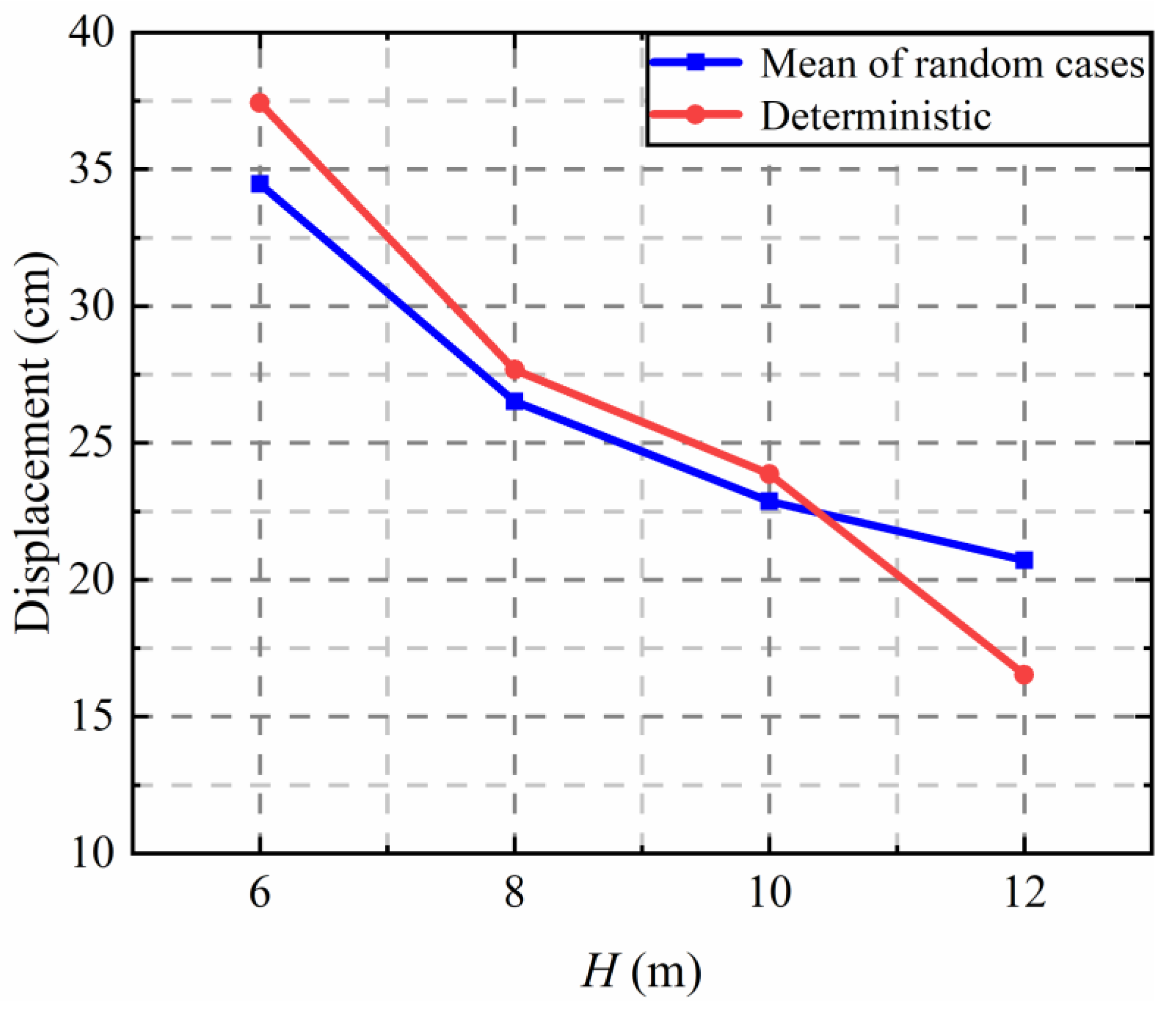
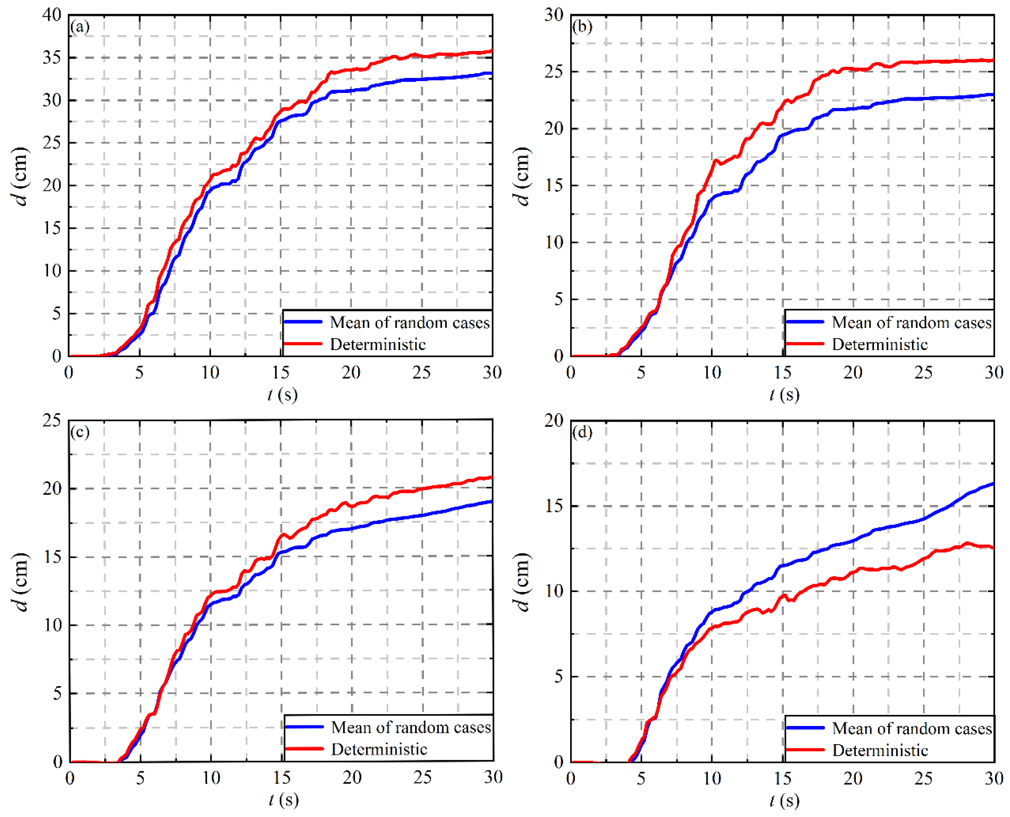
4.3. Effect of Tunnel Embedment Depth on Tunnel Displacement

In this section, the displacement responses of the tunnel under different embedment depths under both deterministic and stochastic conditions are calculated. Figure 11 shows the comparison of the time history curve of the uplift displacement of the tunnel under different embedment depths. As can be seen from Figure 11a–c, when the embedment depth of the rectangular tunnel is not more than 10 m, the mean value of uplift displacement of the tunnel obtained by 200 random calculations is smaller than that obtained by deterministic calculations. When the tunnel embedment depth is 6 m, the maximum uplift displacement of the tunnel obtained by the deterministic calculation is 37.42 cm, and the maximum uplift displacement of the tunnel obtained by random analysis is 34.46 cm, which is 7.9% lower than the deterministic calculation. When the tunnel embedment depths are 8 m and 12 m, the gap is reduced to 4.2% and 4.1%, respectively. As the embedment depth of the tunnel continues to increase, when H = 12 m, the mean value of the maximum uplift displacement of the tunnel by random analysis exceeds the deterministic calculated displacement value under this embedment depth. This may be owing to the liquefaction degree of the soil above the tunnel considering spatial variability was less affected when the tunnel was located deep in the foundation, which was beneficial to the uplift of tunnel compared with the deterministic case. The above phenomena indicate that, with the increase of tunnel embedment depth, the safety and reliability of underground structures, such as tunnels, will be lower when the foundation soil is regarded as a uniform material to analyze the uplift displacement response of tunnels and other underground structures due to liquefaction.

The comparison between the stochastic and deterministic analyses of the time history of tunnel uplift displacement under different embedment depths is illustrated in Figure 12. The maximum uplifts of tunnel buried in various embedment depths in the deterministic case given in Figure 12b is consistent with the study of Liu and Song [19], which can be described as the increase of buried depth reduces the uplift of underground structures in liquefiable soil. Accordingly, the mean values of stochastic cases illustrated in Figure 12a have the same tendency. The reason is that the thickness of the overlying soil above the tunnel increases with the embedment depth of the tunnel. The soil gravity induced vertical force applied to the tunnel increases, since the parameters of the whole model soil are the same. The resistance force against the tunnel uplift displacement increases, resulting in the decrease of the tunnel uplift displacement.

In order to further analyze the influence of tunnel embedment depth on the uplift displacement, the maximum uplift displacement of the tunnel is calculated, as shown in Figure 13. As can be seen from the figure, the maximum uplift displacement value of the tunnel is approximately in line with the tunnel embedment depth in the range of 8 m to 12 m. However, under the shear modulus random field model with variation coefficient COV = 0.3 and horizontal and vertical fluctuation ranges of 50 m and 10 m, respectively, the decreasing rate of the mean displacement of the tunnel with the increase of the embedment depth of the random analysis is greater than that calculated in the deterministic condition of uniform soil field.

Figure 14 and Figure 15 show the probability density function (PDF) curves and cumulative distribution function (CDF) of the peak value of tunnel uplift displacement at different embedment depths, respectively. As shown in Figure 14, the uplift displacement calculated by deterministic analyses is greater than that obtained from the peak value of the PDF curve for H = 6 m. The uplift displacement calculated by deterministic analyses is still greater than the maximum stochastic displacement calculated by random analyses with the increase of H. The difference between the results from the two analyses is reducing. Until H = 12 m, the tunnel floating displacement corresponding to the peak of the probability density curves exceeds the displacement calculated by deterministic analyses. It is consistent with the variation trend of the mean values of random analyses shown in Figure 14. The peak of the PDF curve gradually moves left with the depth of tunnel depth. It can be explained in view of the probability that tunnel floating displacement is getting smaller. It can be found from the cumulative distribution that the maximum tunnel floating displacement obtained from random analyses has the probability of 21.1%, exceeding the value calculated by deterministic analyses when H = 6 m. This probability increases to 23.1%, 24.9% and 67.3% when H increases to 8 m, 10 m and 12 m, respectively. It shows that reliability under deterministic analyses decreases with tunnel depth.

4.4. Effect of Tunnel Embedment Depth on Ground Displacement

The first reference point is set at the symmetry center of the soil surface directly above the tunnel center axis to study the variation of the maximum ground heave displacement under different coefficients of variation and scales of fluctuation. Another reference point is set at 4 m intervals with the tunnel center axis as the symmetry axis to analyze the variation of vertical ground displacement with the distance from the tunnel center axis.

Figure 16 indicates the comparison of the time history curves of the maximum uplift displacement at different tunnel embedment depths. It can be seen that when the tunnel embedment depth does not exceed 10 m, the mean of the maximum uplift displacement derived from stochastic analysis is smaller than that derived from the deterministic case. When the tunnel embedment depth reaches 12 m, the mean of the maximum uplift displacement is 16.3 cm, which exceeds the deterministic result by 29.4%. The variation of the maximum uplift displacement with the embedment depth of the tunnel for the stochastic and deterministic analysis is demonstrated in Figure 17. As can be seen from the figure, the uplift displacement located directly above the central axis of the tunnel gradually decreases with the increase of the tunnel embedment depth. The uplift displacement and the top of the tunnel at the same horizontal coordinates at the end of the earthquake are extracted, and the displacement contrasts between the soil and the tunnel are shown in

Table 3. Comparison of maximum vertical displacement between surface and tunnel.

H	6 m	8 m	10 m	12 m
Mean of random cases	96.3%	86.7%	83.1%	78.8%
Deterministic case	95.9%	94.1%	86.8%	76.0%

. It can be found that the maximum uplift of the surface soil is always smaller than the tunnel displacement at different tunnel depths, and the ratio of the maximum uplift of the surface to the tunnel displacement gradually decreases with the increase of the tunnel depth, regardless of whether the spatial variability of the soil shear modulus is considered or not. This is because as the tunnel depth increases, the thickness of the soil layer between the surface and the tunnel increases, and due to the compressibility of the soil, the greater the thickness of the soil layer, the greater the compression under the same dynamic load, resulting in a greater relative reduction of the vertical displacement of the surface.

Figure 18 and Figure 19 show the peak PDF and CDF of vertical surface displacement under different tunnel embedment depths, respectively. It can be seen that with the increase in tunnel depth, the distribution range of the maximum surface displacement gradually shifts to the left. The displacement value corresponding to the peak point of the probability density curve gradually decreases. However, the kurtosis is larger and the displacement distribution is more concentrated. As can be seen from Figure 19, when the embedment depth of the tunnel increases from 6 m to 12 m, the probability of the maximum surface uplift value obtained by random analysis exceeding the deterministic calculation result is 24.9%, 14.7%, 19.9% and 71.6%, respectively. Therefore, if buildings are on the surface above the tunnel, or the requirements for surface settlement are high, it is necessary to consider the spatial variability of soil parameters when analyzing the safety of tunnels and above-ground structures.

Figure 20 shows the comparison of vertical displacements at each position of the ground under different embedment depths of tunnels by deterministic analysis and stochastic analysis. The soil above the tunnel shows uplift displacement, while the settlement deformation occurred in the surface far away from the tunnel. This finding were accordant to the research of Azadi and Hosseini [20]. It can be found that the difference between the displacement mean value of stochastic analysis and the deterministic calculation result is small in the area of surface uplift, while the difference is large in the area of surface settlement far from the tunnel structure. With the increase of tunnel embedment depth, the maximum uplift displacement of surface soil decreases continuously, and the maximum settlement also decreases. When the depth of the tunnel is H = 12 m, the difference between the stochastic calculation and the deterministic analysis is the largest, with a difference of 28.8%. The largest difference in surface subsidence occurs when H = 6 m, which is 67.9%. It can be explained that the spatial variability of soil far from the tunnel was less reduced by the averaging effect of tunnel.

Figure 21 shows a set of random analysis of seismic vertical displacement contours for tunnel embedment depth H = 6 m. As can be found from the figure, after the earthquake effect, the foundation is in different degrees of liquefaction, leading to the surface of the tunnel structure, squeezing soil above the tunnel and, at the same time, making the soil around the tunnel supplement the bottom of the region. As illustrated by Mahmoud et al. [18], it is an imbalance of vertical pressures arising from the development of excess pore water pressure beneath the underground structures that leads to the underground structures uplift, which is accompanied by the surrounding soil settlement as a result of the soil movement, which is consistent with the results of this study. From the displacement vector diagram of soil around the tunnel shown in Figure 22, it can be more intuitively seen that the soil above the tunnel is squeezed and moves away from the tunnel area, while the soil on both sides forms a circular displacement trajectory to complement the lower part of the tunnel. A similar phenomenon was also revealed by Kang et al. [51], that the displacement vectors were directed toward the bottom of the structure. In addition, Chian et al. [52] illustrated that soil deformation around the circular tunnel formed wide circular loops on both sides of the structure, displacing soil from the crown to the invert of the structure. However, Bao et al. [21] presented that the soil deformation around the structure did not form wide circular loops at the two sides of the structure, which may be attributed to the rectangular shape of the metro tunnel. The greater the depth of the tunnel, the thicker the upper floating soil layer; the greater the resistance to its upward movement, the smaller the corresponding upward displacement and surface uplift of the tunnel; and the less soil needed to replenish beneath the tunnel, the smaller the settlement of the soil in the area away from the tunnel.

5. Conclusions

In this study, dynamic response characteristics of foundation soil and tunnel structure were studied under four kinds of tunnel depth conditions by considering soil anisotropy random field, including the analysis of soil excess pore water pressure ratio, foundation liquefaction range, tunnel floating displacement and surface deformation. Based on the results of calculation and analysis, the main conclusions were as follows:

(1)

The excessive static pore pressure ratio and soil liquefaction range are greatly affected by the change in the tunnel embedment depth. With depth increasing, the soil excess pore water pressure ratio under the tunnel gradually decreases and the liquefaction degree reduces. The peak value of the foundation liquefaction range increases with the increase of embedment depth, and the time history of the liquefaction range rises faster over time in the ascending stage, while decreasing faster over time in the descending stage.

(2)

The tunnel depth has the same effect on the maximum uplift displacement of the tunnel and the ground surface. With the increase of embedment depth, the thickness of the overlying soil and the gravity of the soil also increase, which leads to the decrease of the maximum displacement of the tunnel and the ground surface, and the decrease of the maximum settlement of soil far away from the tunnel area.

(3)

When considering the anisotropy random fields of soil shear modulus, the mean response of stochastic analysis is smaller than the deterministic calculation results when the tunnel embedment depth is less than 10 m. However, when H = 10 m, it will seriously overestimate the deformation of soil and tunnel structure if the soil is regarded as a uniform field.

The conclusions obtained in this paper are able to provide guidance for the site selection and seismic design of tunnels in the liquefaction zone. The limitations of the study primarily exist in two aspects: firstly, only one type of random field was adopted in this paper, the effect of the coefficients of variation and scales of fluctuation of random field on the tunnel behavior had not been studied; secondly, the plane strain condition was adopted in this paper, while the seismic response of the tunnel in the longitudinal direction also need to be studied. Further study is recommended to develop a 3-D random field model to investigate the dynamic response of tunnels in the longitudinal direction.

References

1. Hamada, M.; Isoyama, R.; Wakamatsu, K. Liquefaction-induced ground displacement and its related damage to lifeline facilities. Soils Found 1996, 36, 81–97. [Google Scholar] [CrossRef]
2. Uenishi, K.; Sakurai, S. Characteristic of the vertical seismic waves associated with the 1995 Hyogo-ken Nanbu (Kobe), Japan earthquake estimated from the failure of the Daikai Underground Station. Earthq. Eng. Struct. Dyn. 2000, 29, 813–821. [Google Scholar] [CrossRef]
3. Wang, W.L.; Wang, T.T.; Su, J.J.; Lin, C.H.; Seng, C.R.; Huang, T.H. Assessment of damage in mountain tunnels due to the Taiwan Chi-Chi Earthquake. Tunn. Undergr. Space Technol. 2001, 16, 133–150. [Google Scholar] [CrossRef]
4. Chou, H.S.; Yang, C.Y.; Hsieh, B.J.; Chang, S.S. A study of liquefaction related damages on shield tunnels. Tunn. Undergr. Space Technol. 2001, 16, 185–193. [Google Scholar] [CrossRef]
5. Wang, Z.Z.; Zhang, Z. Seismic damage classification and risk assessment of mountain tunnels with a validation for the 2008 Wenchuan earthquake. Soil Dyn. Earthq. Eng. 2013, 45, 45–55. [Google Scholar] [CrossRef]
6. Miao, Y.; He, H.J.; Liu, H.B.; Wang, S.Y. Reproducing ground response using in-situ soil dynamic parameters. Earthq. Eng. Struct Dyn. 2022, 51, 2449–2465. [Google Scholar] [CrossRef]
7. Chen, G.X.; Chen, S.; Qi, C.Z.; Du, X.L.; Wang, Z.H.; Chen, W.Y. Shaking table tests on a three-arch type subway station structure in a liquefiable soil. Bull. Earthq. Eng. 2015, 13, 1675–1701. [Google Scholar] [CrossRef]
8. Yu, H.T.; Yan, X.; Bobet, A.; Yuan, Y.; Xu, G.P.; Su, Q.K. Multi-point shaking table test of a long tunnel subjected to non-uniform seismic loadings. Bull. Earthq. Eng. 2018, 16, 1041–1059. [Google Scholar] [CrossRef]
9. Hou, C.; Jin, X.G.; Ge, Y.; He, J. Shaking table test on the seismic response of a frame-type subway station in composite soil. Int. J. Geomech. 2021, 21, 04021220. [Google Scholar] [CrossRef]
10. Chian, S.C.; Madabhushi, S.P.G. Effect of embedment depth and diameter on uplift of underground structures in liquefied soils. Soil Dyn. Earthq. Eng. 2012, 41, 181–190. [Google Scholar] [CrossRef]
11. Lanzano, G.; Bilotta, E.; Russo, G.; Silvestri, F. Experimental and numerical study on circular tunnels under seismic loading. Eur. J. Environ. Civ. Eng. 2015, 19, 539–563. [Google Scholar] [CrossRef]
12. Zhang, Z.H.; Li, Y.; Xu, C.S.; Du, X.L.; Dou, P.F.; Yan, G.Y. Study on seismic failure mechanism of shallow embedment underground frame structures based on dynamic centrifuge tests. Soil Dyn. Earthq. Eng. 2021, 150, 106938. [Google Scholar] [CrossRef]
13. Yu, H.T.; Chen, J.T.; Bobet, A.; Yuan, Y. Damage observation and assessment of the Longxi tunnel during the Wenchuan earthquake. Tunn. Undergr. Space Technol. 2016, 54, 102–116. [Google Scholar] [CrossRef]
14. Miao, Y.; Yao, E.L.; Ruan, B.; Zhuang, H.Y. Seismic response of shield tunnel subjected to spatially varying earthquake ground motions. Tunn. Undergr. Space Technol. 2018, 77, 216–226. [Google Scholar] [CrossRef]
15. Banerjee, S.K.; Chakraborty, D. Stability analysis of a circular tunnel underneath a fully liquefied soil layer. Tunn. Undergr. Space Technol. 2018, 78, 84–94. [Google Scholar] [CrossRef]
16. Azadi, M.; Hosseini, S.M.M.M. The uplifting behavior of shallow tunnels within the liquefiable soils under cyclic loadings. Tunn. Undergr. Space Technol. 2010, 25, 158–167. [Google Scholar] [CrossRef]
17. Song, K.I.; Cho, G.C.; Lee, S.W. Effects of spatially variable weathered rock properties on tunnel behavior. Probabilistic Eng. Mech. 2011, 26, 413–426. [Google Scholar] [CrossRef]
18. Mahmoud, A.O.; Hussien, M.N.; Karray, M.; Chekired, M.; Bessette, C.; Jinga, L. Mitigation of liquefaction-induced uplift of underground structures. Comput. Geotech. 2020, 125, 103663. [Google Scholar] [CrossRef]
19. Liu, H.B.; Song, E.R. Seismic response of large underground structures in liquefiable soils subjected to horizontal and vertical earthquake excitations. Comput. Geotech. 2005, 32, 223–244. [Google Scholar] [CrossRef]
20. Azadi, M.; Hosseini, S.M.M.M. Analyses of the effect of seismic behavior of shallow tunnels in liquefiable grounds. Tunn. Undergr. Space Technol. 2010, 25, 543–552. [Google Scholar] [CrossRef]
21. Bao, X.H.; Xia, Z.F.; Ye, G.L.; Fu, Y.B.; Su, D. Numerical analysis on the seismic behavior of a large metro subway tunnel in liquefiable ground. Tunn. Undergr. Space Technol. 2017, 66, 91–106. [Google Scholar] [CrossRef]
22. Zheng, G.; Yang, P.B.; Zhou, H.Z.; Zeng, C.F.; Yang, X.Y.; He, X.P.; Yu, X.X. Evaluation of the earthquake induced uplift displacement of tunnels using multivariate adaptive regression splines. Comput. Geotech. 2019, 113, 103099. [Google Scholar] [CrossRef]
23. Huang, H.W.; Xiao, L.; Zhang, D.M.; Zhang, J. Influence of spatial variability of soil Young’s modulus on tunnel convergence in soft soils. Eng. Geol. 2017, 228, 357–370. [Google Scholar] [CrossRef]
24. Li, K.S.; Lumb, P. Probabilistic design of slopes. Can. Geotech. J. 1987, 24, 520–535. [Google Scholar] [CrossRef]
25. Zhang, J.; Zhang, L.M.; Tang, W.H. New methods for system reliability analysis of soil slopes. Can. Geotech. J. 2011, 48, 1138–1148. [Google Scholar] [CrossRef]
26. Cho, S.E. Probabilistic stability analysis of rainfall-induced landslides considering spatial variability of permeability. Eng. Geol. 2014, 171, 11–20. [Google Scholar] [CrossRef]
27. Shu, S.; Ge, B.; Wu, Y.X.; Zhang, F. Probabilistic assessment on 3D stability and failure mechanism of undrained slopes. Int. J. Geomech. 2022; accepted. [Google Scholar] [CrossRef]
28. Li, L.; Li, J.H.; Huang, J.S.; Liu, H.J.; Cassidy, M.J. The bearing capacity of spudcan foundations under combined loading in spatially variable soils. Eng. Geol. 2017, 227, 139–148. [Google Scholar] [CrossRef]
29. Wu, Y.X.; Zhou, X.H.; Gao, Y.F.; Shu, S. Bearing capacity of embedment shallow foundations in spatially random soils with linearly increasing mean undrained shear strength. Comput. Geotech. 2020, 122, 103508. [Google Scholar] [CrossRef]
30. Shu, S.; Gao, Y.F.; Wu, Y.X. Probabilistic bearing capacity analysis of spudcan foundation in soil with linearly increasing mean undrained shear strength. Ocean Eng. 2020, 204, 106800. [Google Scholar] [CrossRef]
31. Wu, Y.X.; Zhang, H.L.; Shu, S. Probabilistic bearing capacity of spudcan foundations under combined loading in spatially variable soils. Ocean Eng. 2022, 248, 110738. [Google Scholar] [CrossRef]
32. Constantinou, M.C.; Gazetas, G.; Tadjbakhsh, I. Stochastic seismic sliding of rigid mass supported through non-symmetric friction. Earthq. Eng. Struct. Dyn. 1984, 12, 777–794. [Google Scholar] [CrossRef]
33. Mollon, G.; Dias, D.; Soubra, A.H. Probabilistic analyses of tunneling-induced ground movements. Acta Geotech. 2013, 8, 181–199. [Google Scholar] [CrossRef] [Green Version]
34. Eshraghi, A.; Zare, S. Face stability evaluation of a TBM-driven tunnel in heterogeneous soil using a probabilistic approach. Int. J. Geomech. 2015, 15, 04014095. [Google Scholar] [CrossRef]
35. Miro, S.; Konig, M.; Hartmann, D.; Schanz, T. A probabilistic analysis of subsoil parameters uncertainty impacts on tunnel-induced ground movements with a back-analysis study. Comput. Geotech. 2015, 68, 38–53. [Google Scholar] [CrossRef]
36. Wu, Y.X.; Bao, H.; Wang, J.C.; Gao, Y.F. Probabilistic analysis of tunnel convergence on spatially variable soil: The importance of distribution type of soil properties. Tunn. Undergr. Space Technol. 2021, 109, 103747. [Google Scholar] [CrossRef]
37. Zhang, J.Z.; Huang, H.W.; Zhang, D.M.; Zhou, M.L.; Tang, C.; Liu, D.J. Effect of ground surface surcharge on deformational performance of tunnel in spatially variable soil. Comput. Geotech. 2021, 136, 104229. [Google Scholar] [CrossRef]
38. Chen, Q.S.; Wang, C.F.; Juang, C.H. CPT-Based Evaluation of Liquefaction Potential Accounting for Soil Spatial Variability at Multiple Scales. J. Geotech. Geoenviron. 2016, 142, 04015077. [Google Scholar] [CrossRef]
39. Wang, C.F.; Chen, Q.S.; Shen, M.F.; Juang, C.H. On the spatial variability of CPT-based geotechnical parameters for regional liquefaction evaluation. Soil Dyn. Earthq. Eng. 2017, 95, 153–166. [Google Scholar] [CrossRef]
40. Juang, C.H.; Shen, M.F.; Wang, C.F.; Chen, Q.S. Random field-based regional liquefaction hazard mapping-data inference and model verification using a synthetic digital soil field. Bull. Eng. Geol. Environ. 2018, 77, 1273–1286. [Google Scholar] [CrossRef]
41. Kim, H.S.; Kim, M.; Baise, L.G.; Kim, B. Local and regional evaluation of liquefaction potential index and liquefaction severity number for liquefaction-induced sand boils in pohang, South Korea. Soil Dyn. Earthq. Eng. 2021, 141, 106459. [Google Scholar] [CrossRef]
42. Wang, Y.B.; Shu, S.; Wu, Y.X. Reliability Analysis of Soil Liquefaction Considering Spatial Variability of Soil Property. J. Earthq. Tsunami 2021, 16, 2250002. [Google Scholar] [CrossRef]
43. Wang, Y.B.; He, J.J.; Shu, S.; Zhang, H.L.; Wu, Y.X. Seismic responses of rectangular tunnels in liquefiable soil considering spatial variability of soil properties. Soil Dyn. Earthq. Eng. 2022, 162, 107489. [Google Scholar] [CrossRef]
44. Ali, A.; Lyamin, A.V.; Huang, J.S.; Sloan, S.W.; Cassidy, M.J. Undrained stability of a single circular tunnel in spatially variable soil subjected to surcharge load. Comput. Geotech. 2017, 84, 16–27. [Google Scholar] [CrossRef]
45. Gong, W.P.; Juang, C.H.; Martin, J.R.; Tang, H.M.; Wang, Q.Q.; Huang, H.W. Probabilistic analysis of tunnel longitudinal performance based upon conditional random field simulation of soil properties. Tunn. Undergr. Space Technol. 2018, 73, 1–14. [Google Scholar] [CrossRef]
46. Popescu, R.; Deodatis, G.; Nobahar, A. Effects of random heterogeneity of soil properties on bearing capacity. Probabilistic Eng. Mech. 2005, 20, 324–341. [Google Scholar] [CrossRef]
47. Popescu, R.; Deodatis, G.; Prevost, J.H. Simulation of non-Gaussian homogeneous stochastic vector fields. Probabilistic Eng. Mech. 1998, 13, 1–13. [Google Scholar] [CrossRef]
48. Wu, Y.X.; Li, R.; Gao, Y.F.; Zhang, N.; Zhang, F. Simple and efficient method to simulate homogenous multidimensional non-Gaussian vector field by the spectral representation method. J. Eng. Mech. 2017, 143, 06017016. [Google Scholar] [CrossRef]
49. Stefanou, G.; Papadrakakis, M. Assessment of spectral representation and Karhunen-Loeve expansion methods for the simulation of Gaussian stochastic fields. Comput. Methods App. Mech. Eng. 2007, 196, 2465–2477. [Google Scholar] [CrossRef]
50. Zheng, G.; Yang, P.B.; Zhou, H.Z.; Zhang, W.B. The uplift response of rectangular tunnel in liquefiable soil. China Civ. Eng. J. 2019, 52, 257–264. [Google Scholar]
51. Kang, G.C.; Tobita, T.; Iai, S. Seismic simulation of liquefaction-induced uplift behavior of a hollow cylinder structure buried in shallow ground. Soil Dyn. Earthq. Eng. 2014, 64, 85–94. [Google Scholar] [CrossRef]
52. Chian, S.C.; Tokimatsu, K.; Madabhushi, S.P.G. Soil liquefaction-induced uplift of underground structures: Physical and numerical modeling. J. Geotech. Geoenviron. 2014, 140, 04014057. [Google Scholar] [CrossRef]
Figure 1. The tunnel with an embedment depth of 6 m.
Applsci 12 10719 g001
Figure 2. Time history of earthquake acceleration.
Applsci 12 10719 g002
Figure 3. Typical random field realization of soil shear modulus.
Applsci 12 10719 g003
Figure 4. Layout of monitoring points when the tunnel is embedment at a depth of 6 m.
Applsci 12 10719 g004
Figure 5. Comparison of the EPWP ratio under different embedment depths at Point A: (a) H = 6 m; (b) H = 8 m; (c) H = 10 m; (d) H = 12 m.
Applsci 12 10719 g005
Figure 6. Influence of the tunnel embedment depths on the EPWP ratio at Point A.
Applsci 12 10719 g006
Figure 7. Variation of A80 with time history under different embedment depths of tunnel: (a) H = 6 m; (b) H = 8 m; (c) H = 10 m; (d) H = 12 m.
Applsci 12 10719 g007
Figure 8. Comparison of mean time history of ground liquefaction range under different embedment depths.
Applsci 12 10719 g008
Figure 9. PDF of liquefaction range for different embedment depths.
Applsci 12 10719 g009
Figure 10. Cumulative distribution function (CDF) of A80 under different embedment depths of tunnel.
Applsci 12 10719 g010
Figure 11. Comparison of time history curve of the uplift displacement of the tunnel under different embedment depths: (a) H = 6 m; (b) H = 8 m; (c) H = 10 m; (d) H = 12 m.
Applsci 12 10719 g011
Figure 12. Comparison between the stochastic and deterministic analyses of the time history of tunnel uplift displacement: (a) random cases; (b) deterministic cases.
Applsci 12 10719 g012
Figure 13. The maximum uplift displacement of the tunnel under different embedment depths.
Applsci 12 10719 g013
Figure 14. PDF of the peak value of tunnel uplift displacement at different embedment depths: (a) H = 6 m; (b) H = 8 m; (c) H = 10 m; (d) H = 12 m.
Applsci 12 10719 g014
Figure 15. CDF of the peak value of tunnel uplift displacement at different embedment depths: (a) H = 6 m; (b) H = 8 m; (c) H = 10 m; (d) H = 12 m.
Applsci 12 10719 g015
Figure 16. Comparison of time history curve of the upward displacement of the tunnel under different embedment depths: (a) H = 6 m; (b) H = 8 m; (c) H = 10 m; (d) H = 12 m.
Applsci 12 10719 g016
Figure 17. Variation of the maximum uplift displacement with the embedment depth of the tunnel for the stochastic and deterministic analysis: (a) Mean of random cases; (b) deterministic case.
Applsci 12 10719 g017
Figure 18. PDF of the peak value of vertical surface displacement at different embedment depths: (a) H = 6 m; (b) H = 8 m; (c) H = 10 m; (d) H = 12 m.
Applsci 12 10719 g018
Figure 19. CDF of the peak value of vertical surface displacement at different embedment depths: (a) H = 6 m; (b) H = 8 m; (c) H = 10 m; (d) H = 12 m.
Applsci 12 10719 g019
Figure 20. Comparison of vertical displacements at each position of the ground under different embedment depths: (a) H = 6 m; (b) H = 8 m; (c) H = 10 m; (d) H = 12 m.
Applsci 12 10719 g020
Figure 21. The contour of displacement at the embedment depth of 6 m.
Applsci 12 10719 g021
Figure 22. Displacement vector diagram of soil around tunnel structure.
Applsci 12 10719 g022