
Task-Based Motion Planning Using Optimal Redundancy for a Minimally Actuated Robotic Arm
Abstract
1. Introduction
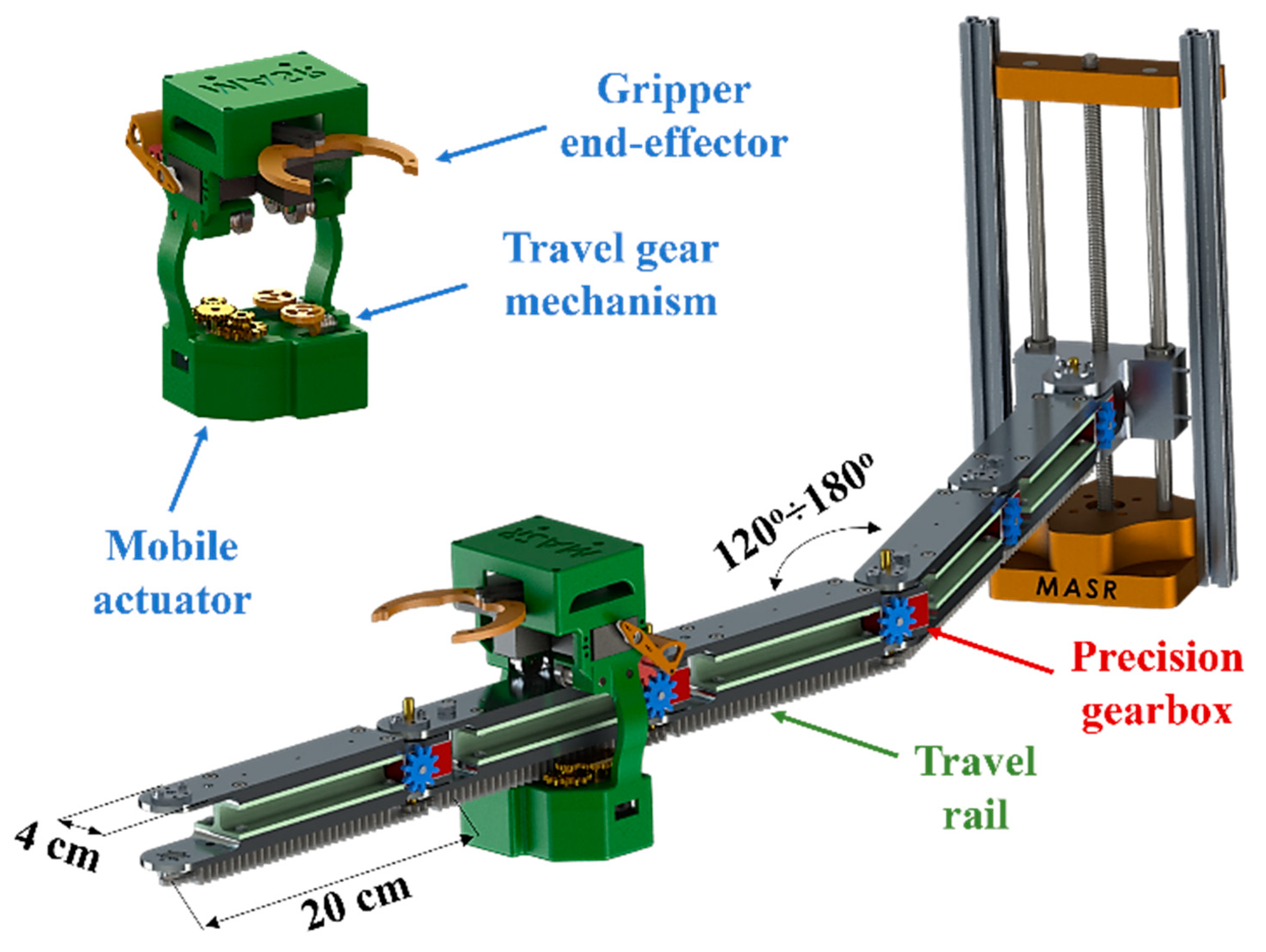
2. MASR Mechanical Characteristics
3. Workspace Analysis
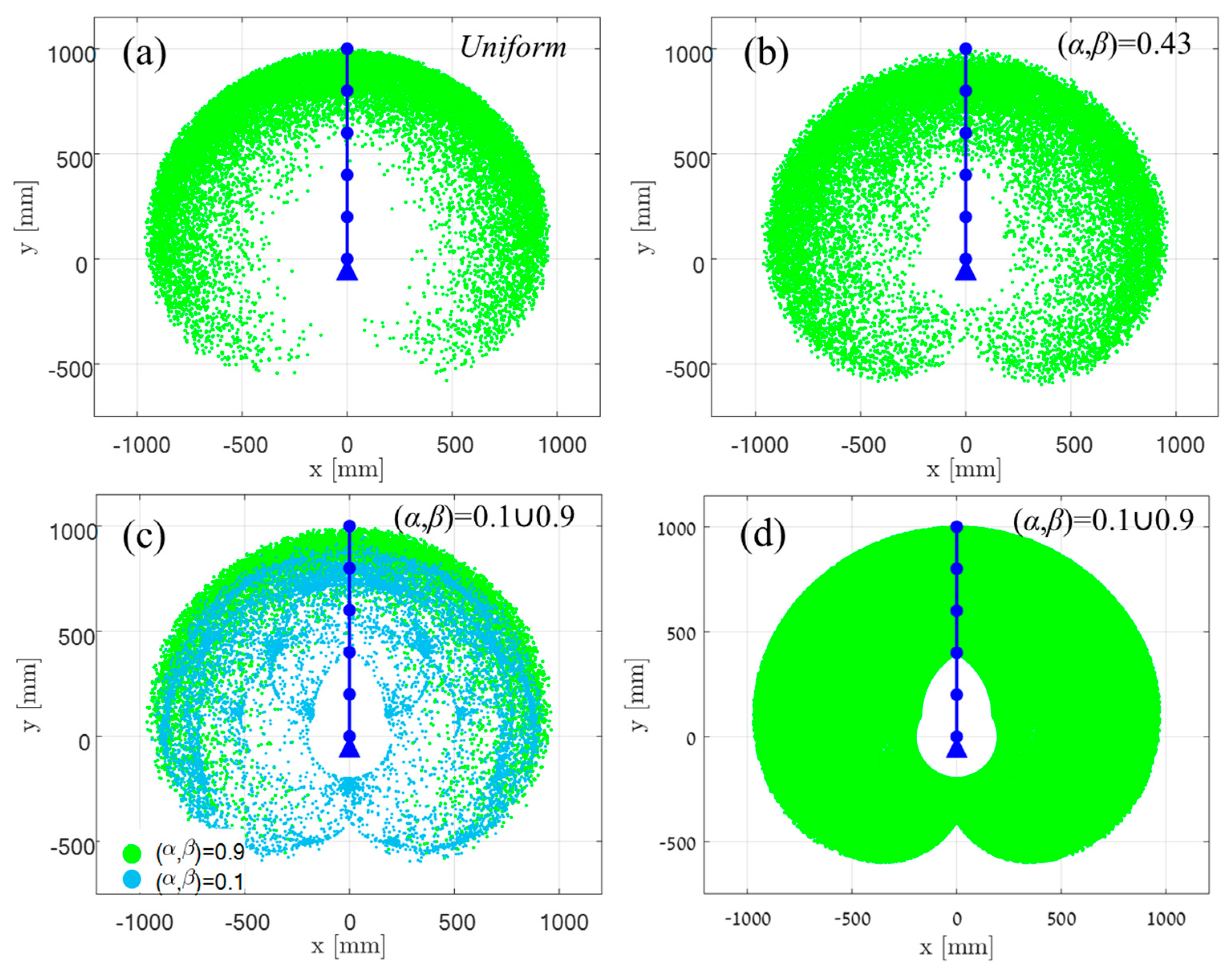
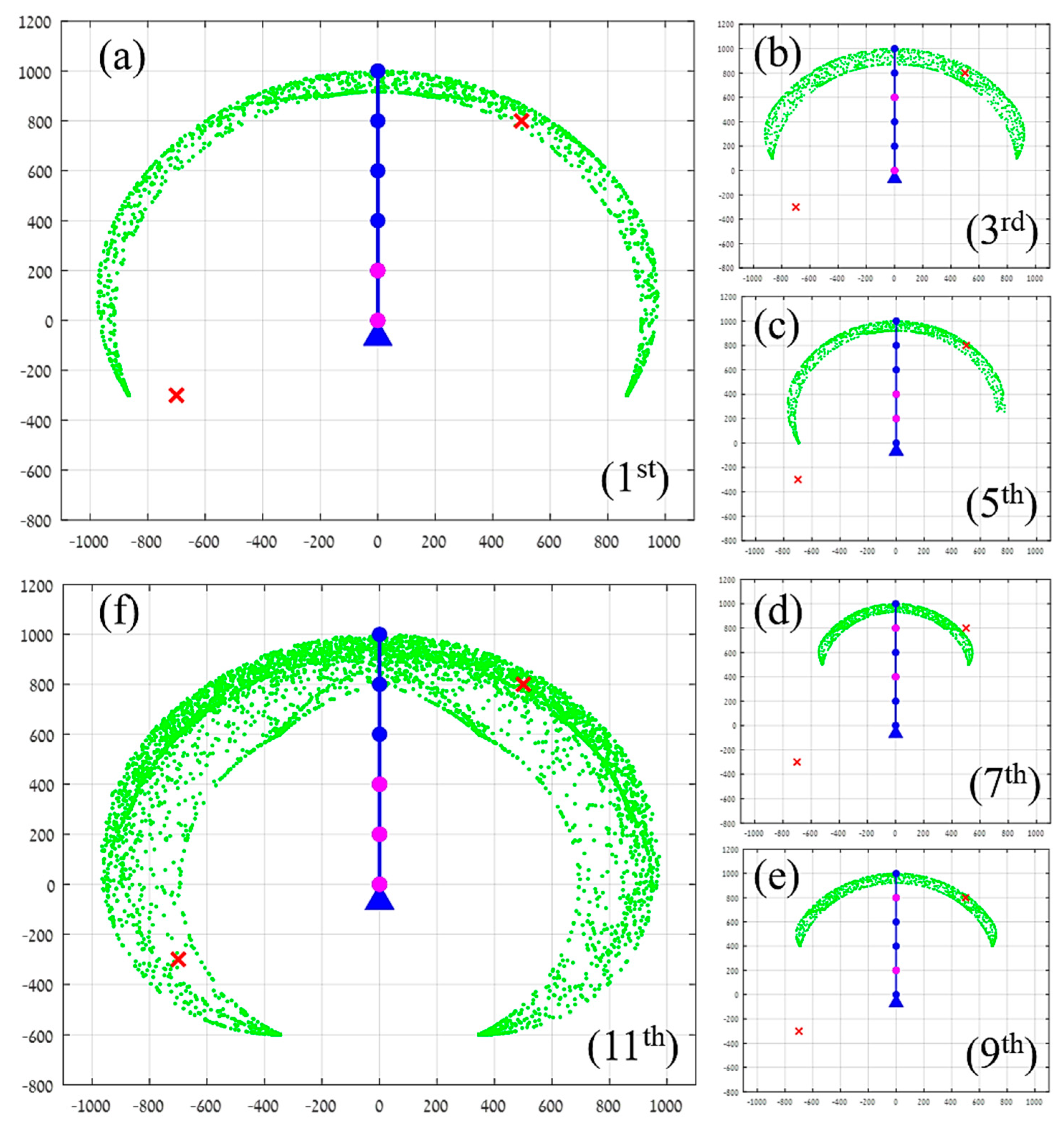
3.1. Workspace Computation
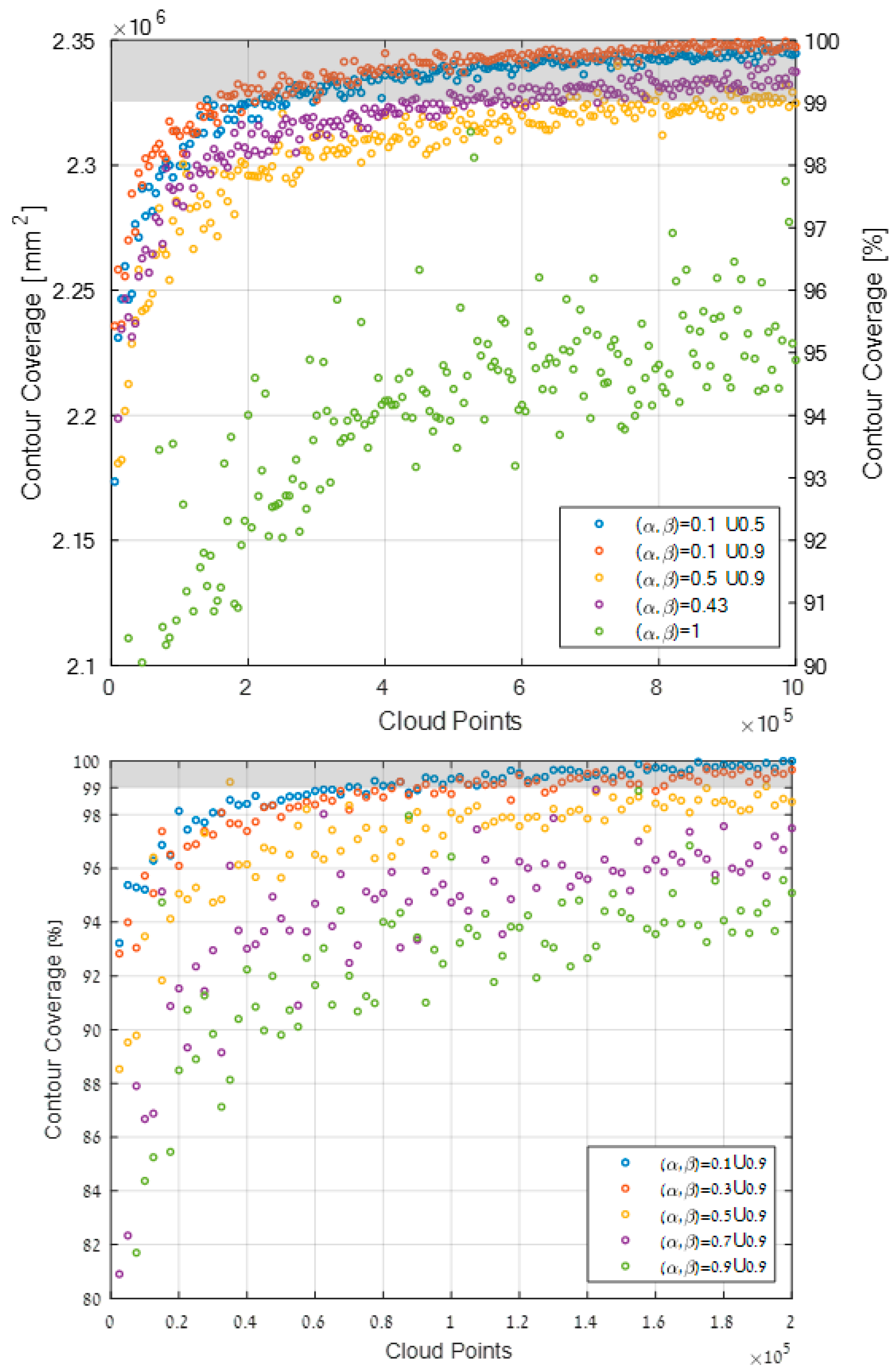
3.2. Contour Coverage
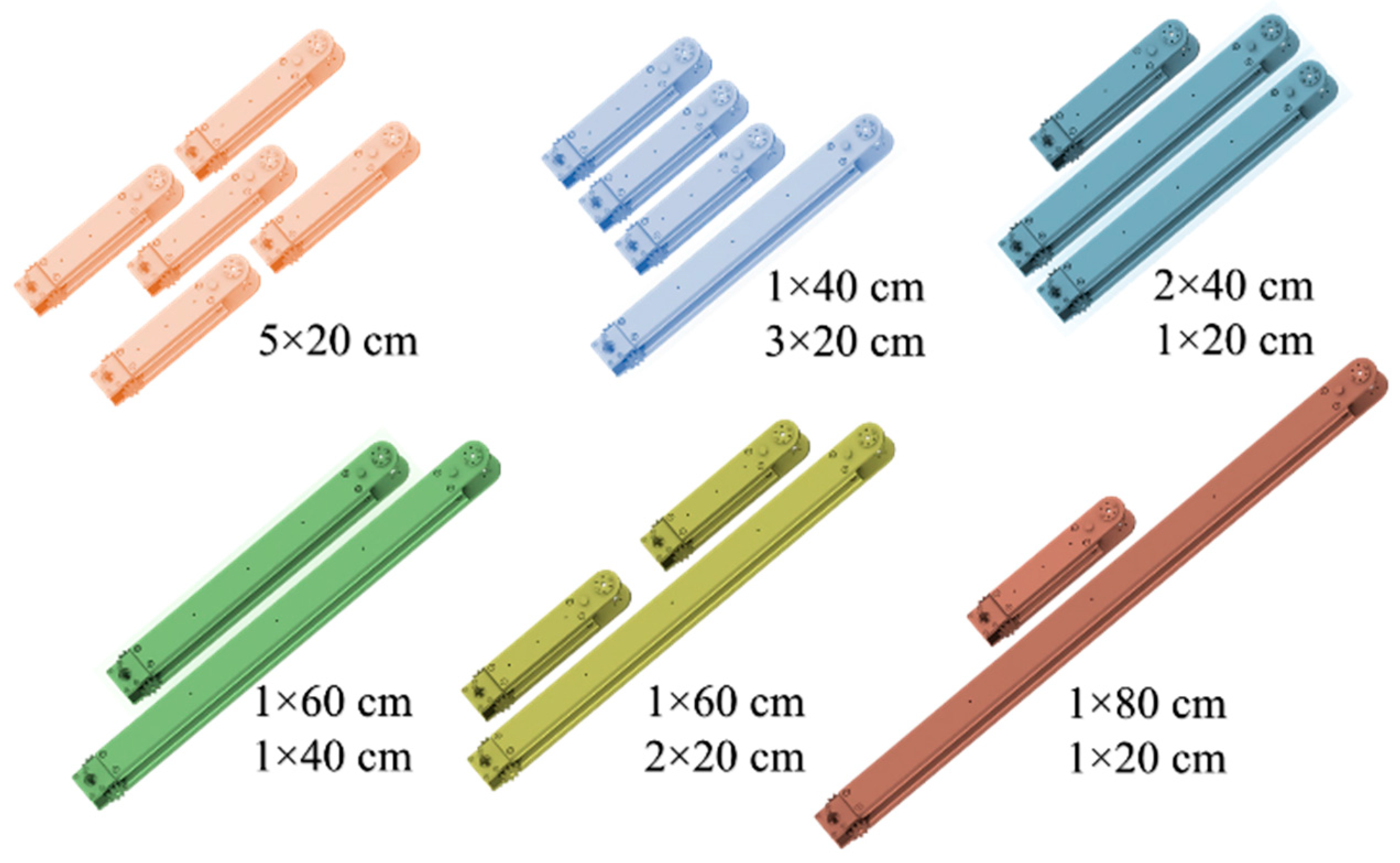
3.3. Optimal Link-Joint Assembly
3.4. Last Link and Any Link Workspace
4. Motion Planning
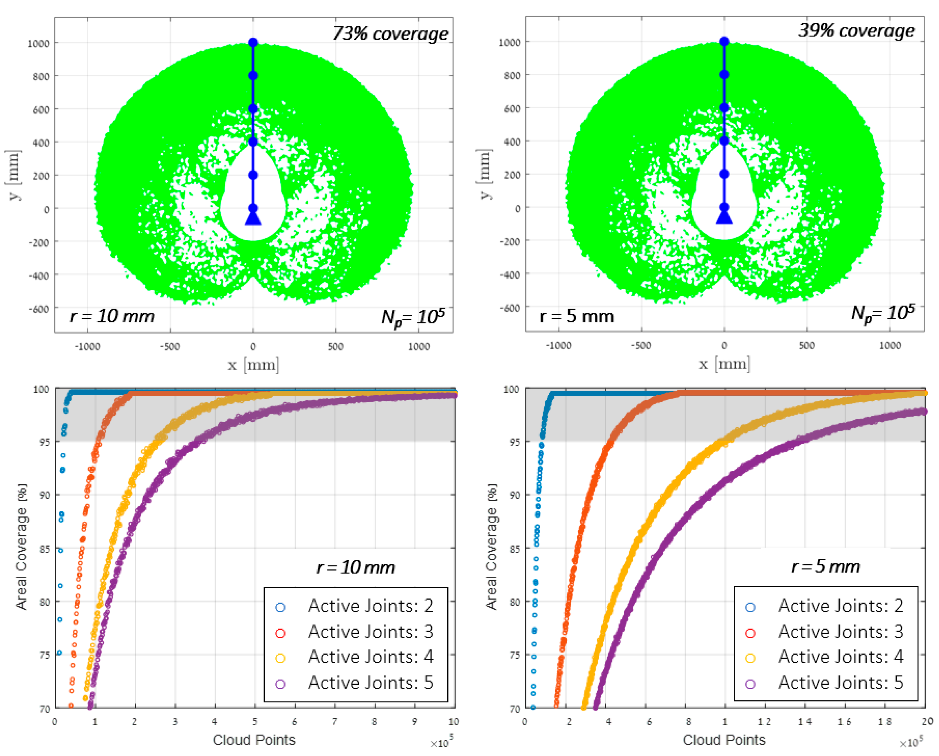
4.1. Areal Coverage
4.2. Heuristic Search
5. Simulation Results
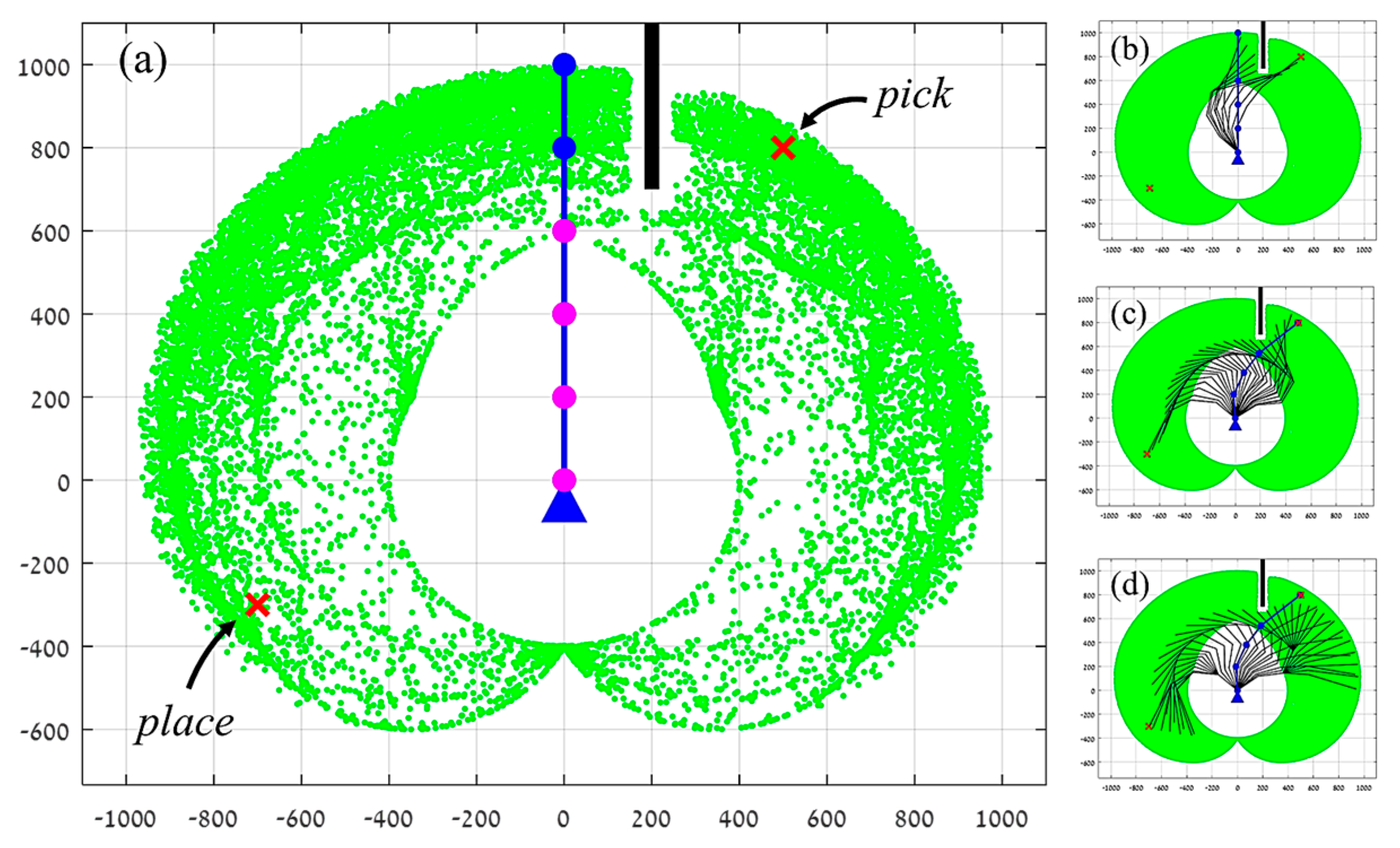
5.1. Pick and Place
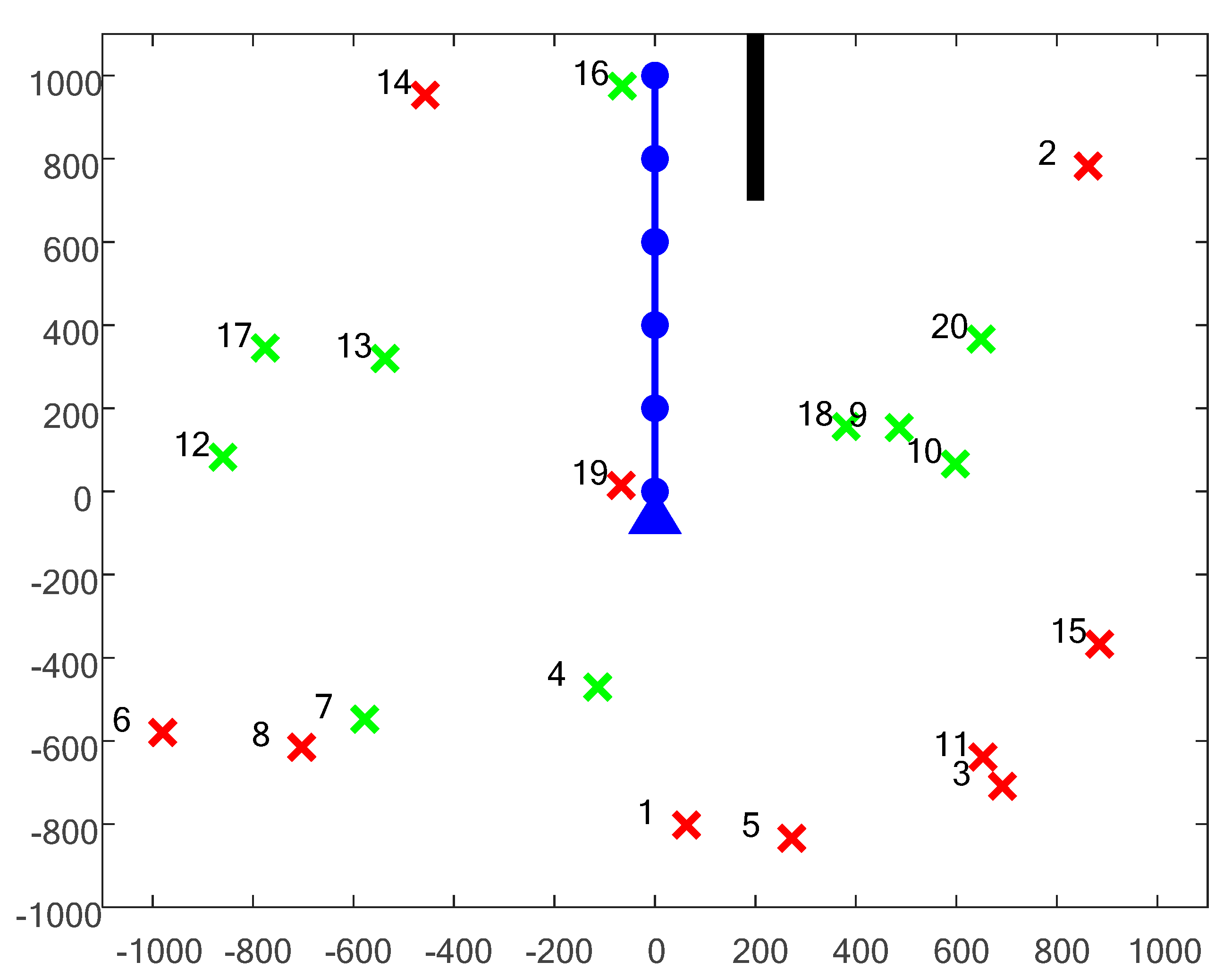
5.2. Last Link vs. Any Link
6. Conclusions
Author Contributions
Funding
Conflicts of Interest
References
- Siciliano, B.; Khatib, O. Springer Handbook of Robotics; Springer: Berlin/Heidelberg, Germany, 2016. [Google Scholar]
- Burgner-Kahrs, J.; Rucker, D.C.; Choset, H. Continuum Robots for Medical Applications: A Survey. IEEE Trans. Robot. 2015, 31, 1261–1280. [Google Scholar] [CrossRef]
- Shao, L.; Guo, B.; Wang, Y.; Chen, X. An overview on theory and implementation of snake-like robots. In Proceedings of the 2015 IEEE International Conference on Mechatronics and Automation (ICMA 2015), Beijing, China, 2–5 August 2015. [Google Scholar]
- Menon, M.S.; Ravi, V.C.; Ghosal, A. Trajectory planning and obstacle avoidance for hyper-redundant serial robots. J. Mech. Robot. 2017, 9, 041010. [Google Scholar] [CrossRef]
- El-Sherbiny, A.; Elhosseini, M.A.; Haikal, A.Y. A comparative study of soft computing methods to solve inverse kinematics problem. Ain Shams Eng. J. 2018, 9, 2535–2548. [Google Scholar] [CrossRef]
- Reiter, A. Path and Trajectory Planning. In Optimal Path and Trajectory Planning for Serial Robots; Springer Vieweg: Wiesbaden, Germany, 2020. [Google Scholar]
- Moubarak, P.; Ben-Tzvi, P. Modular and reconfigurable mobile robotics. Robot. Auton. Syst. 2012, 60, 1648–1663. [Google Scholar] [CrossRef]
- Yim, M.; Shen, W.-M.; Salemi, B.; Rus, D.; Moll, M.; Lipson, H.; Klavins, E. Modular Self-reconfigurable Robot Systems: Challenges and Opportunities for the Future. IEEE Robot. Autom. Mag. 2007, 14, 43–52. [Google Scholar] [CrossRef]
- Ayalon, Y.; Damti, L.; Zarrouk, D. Design and Modelling of a Minimally Actuated Serial Robot. IEEE Robot. Autom. Lett. 2020, 5, 4899–4906. [Google Scholar] [CrossRef]
- Mann, M.P.; Damti, L.; Tirosh, G.; Zarrouk, D. Minimally actuated serial robot. Robotica 2018, 36, 408–426. [Google Scholar] [CrossRef]
- Cao, Y.; Lu, K.; Li, X.; Zang, Y. Accurate Numerical Methods for Computing 2D and 3D Robot Workspace. Int. J. Adv. Robot. Syst. 2011, 8, 76. [Google Scholar] [CrossRef]
- Goyal, K.; Sethi, D. An Analytical Method to Find Workspace of a Robotic Manipulator. J. Mech. Eng. 1970, 41, 25–30. [Google Scholar] [CrossRef]
- Alciatore, D.G.; Ng, C.C.D. Determining manipulator workspace boundaries using the Monte Carlo method and least squares segmentation. Am. Soc. Mech. Eng. Des. Eng. Div. 1994, 72, 141–146. [Google Scholar]
- Rastegar, J.; Fardanesh, B. Manipulation workspace analysis using the Monte Carlo Method. Mech. Mach. Theory 1990, 25, 233–239. [Google Scholar] [CrossRef]
- Hart, P.E.; Nilsson, N.J.; Raphael, B. Formal Basis for the Heuristic Determination eijj. Syst. Sci. Cybern. 1968, 4, 100–107. [Google Scholar]
- Aine, S.; Swaminathan, S.; Narayanan, V.; Hwang, V.; Likhachev, M. Multi-Heuristic A*. Int. J. Robot. Res. 2016, 35, 224–243. [Google Scholar] [CrossRef]
- Owen, T. Heuristics: Intelligent Search Strategies for Computer Problem Solving. Robotica 1988, 6, 165. [Google Scholar] [CrossRef]
- Cohen, B.; Chitta, S.; Likhachev, M. Single- and dual-arm motion planning with heuristic search. Int. J. Robot. Res. 2014, 33, 305–320. [Google Scholar] [CrossRef]
- Likhachev, M.; Gordon, G.; Thrun, S. ARA*: Anytime A* with Provable Bounds on Sub-Optimality. In Proceedings of the Advances in Neural Information Processing Systems (NIPS 2003), Vancouver, BC, Canada, 8–13 December 2003. [Google Scholar]
- Kanehiro, F.; Yoshimi, T.; Kajita, S.; Morisawa, M.; Kaneko, K.; Hirukawa, H.; Tomita, F. Whole Body Locomotion Planning of Humanoid Robots based on a 3D Grid Map. J. Robot. Soc. Jpn. 2007, 25, 589–597. [Google Scholar] [CrossRef][Green Version]
- Kirkpatrick, D.G.; Seidel, R. On the Shape of a Set of Points in the Plane. IEEE Trans. Inf. Theory 1983, 29, 551–559. [Google Scholar] [CrossRef]
- Pohl, I. Heuristic search viewed as path finding in a graph. Artif. Intell. 1970, 1, 193–204. [Google Scholar] [CrossRef]


| Number of Links | Points to Full Contour Coverage | Reduction | |
|---|---|---|---|
| Superposition (α,β) = 0.1∪0.9 | No Superposition (α,β) = 0.43 | (%) | |
| 2 | 1600 | 4950 | 67.7 |
| 3 | 11,100 | 112,350 | 90.1 |
| 4 | 56,950 | 267,200 | 78.7 |
| 5 | 210,000 | 610,000 | 65.6 |
| 98% Coverage | 95% Coverage | Number of Links | ||||
|---|---|---|---|---|---|---|
| r = 15 mm | r = 10 mm | r = 5 mm | r = 15 mm | r = 10 mm | r = 5 mm | |
| 12K | 27K | 108K | 9K | 20K | 82K | 2 |
| 67K | 148K | 574K | 49K | 111K | 433K | 3 |
| 181K | 384K | 1406K | 117K | 261K | 935K | 4 |
| 282K | 587K | 2061K | 165K | 372K | 1372K | 5 |
| Target No. | Last Link Expansions | Any Link Expansions | LL/AL Ratio |
|---|---|---|---|
| 4 | 152,332 | 27,738 | 5.5 |
| 7 | 10,448 | 11,978 | 0.9 |
| 9 | 34,548 | 11,044 | 3.1 |
| 10 | 74,128 | 10,530 | 7.0 |
| 12 | 4495 | 447 | 10.1 |
| 13 | 1211 | 99 | 12.2 |
| 16 | 4 | 9 | 0.4 |
| 17 | 1851 | 276 | 6.7 |
| 18 | 13,021 | 12,712 | 1.0 |
| 20 | 32,299 | 9693 | 3.3 |
Publisher’s Note: MDPI stays neutral with regard to jurisdictional claims in published maps and institutional affiliations. |
© 2022 by the authors. Licensee MDPI, Basel, Switzerland. This article is an open access article distributed under the terms and conditions of the Creative Commons Attribution (CC BY) license (https://creativecommons.org/licenses/by/4.0/).
Share and Cite
Gal, Y.; Zarrouk, D. Task-Based Motion Planning Using Optimal Redundancy for a Minimally Actuated Robotic Arm. Appl. Sci. 2022, 12, 9526. https://doi.org/10.3390/app12199526
Gal Y, Zarrouk D. Task-Based Motion Planning Using Optimal Redundancy for a Minimally Actuated Robotic Arm. Applied Sciences. 2022; 12(19):9526. https://doi.org/10.3390/app12199526
Chicago/Turabian StyleGal, Yanai, and David Zarrouk. 2022. "Task-Based Motion Planning Using Optimal Redundancy for a Minimally Actuated Robotic Arm" Applied Sciences 12, no. 19: 9526. https://doi.org/10.3390/app12199526
APA StyleGal, Y., & Zarrouk, D. (2022). Task-Based Motion Planning Using Optimal Redundancy for a Minimally Actuated Robotic Arm. Applied Sciences, 12(19), 9526. https://doi.org/10.3390/app12199526