
A Resilient Cyber-Physical Demand Forecasting System for Critical Infrastructures against Stealthy False Data Injection Attacks


Abstract
1. Introduction
2. Related Work
2.1. Definitions
2.2. Challenges in Demand Forecasting
2.3. Overview of Existing Defense Strategies against Stealthy False Data Injection Attacks (FDIAs)
3. Proposed Resilient Demand Forecasting Systems
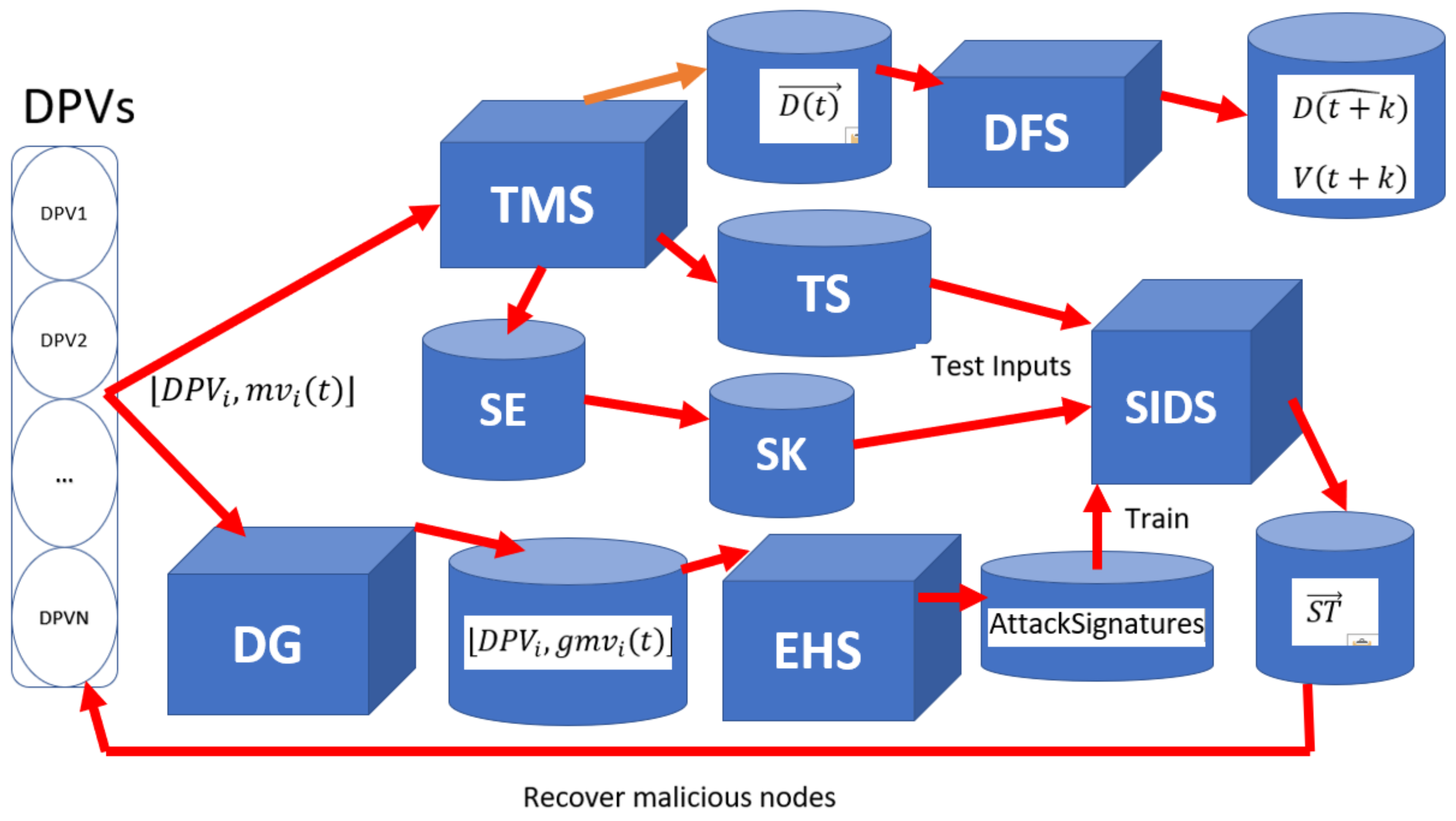
- Present to TMS. TMS estimates the most trustworthy aggregated measurement of demand and sends it to DFS to forecast the k-step ahead demand .
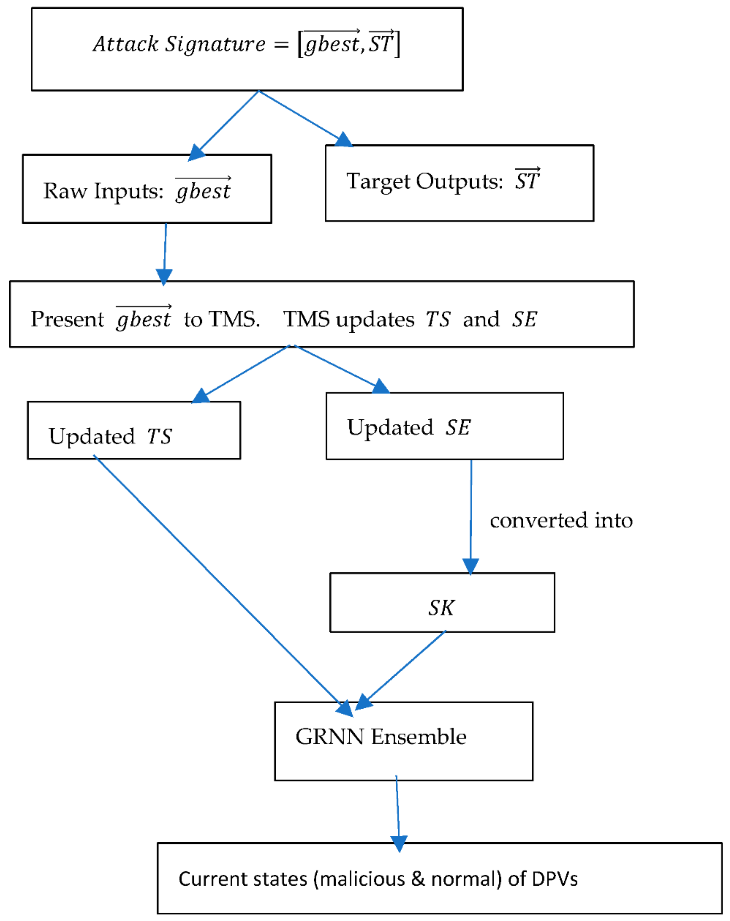
- Present to TMS. TMS estimates the most trustworthy aggregated measurement of demand and sends it to DFS to forecast the k-step ahead demand . TMS also updates the time series of assessed trust scores of DPVs by adding the assessed trust scores of DPVs (found in ) at time step to , as well as the time series of the residuals of one-step ahead forecasts of each DPV’s measurements by adding the residuals of forecasting the measurements of DPVs at time step to . SIDS uses the updated and to predict the current states (malicious and normal) of DPVs.
- If SIDS detects any malicious node correctly, set to zero and change the state(s) of the detected malicious node(s) from malicious to normal in . Else if when the objective is shifting the demand upward or when the objective is shifting the demand downward, set to zero. Else estimate the fitness using the following formula:

4. Research Methodology
4.1. Evaluation Methodology for PRDFS and BRDFS
4.2. Performance Measures
4.2.1. Accuracy in Detecting Malicious Nodes
4.2.2. The Resilience of the Demand Forecasting System in the Face of Ongoing Attack
4.3. Description of the Benchmark Algorithm (BRDFS)
4.3.1. Demand Forecasting System (DFS) of BRDFS
4.3.2. Trust Management System (TMS) of BRDFS
4.3.3. Malicious Node Detection System of BRDFS
Skewness Detector
Correlation Detector ‘CAD’
4.4. Adversary Model
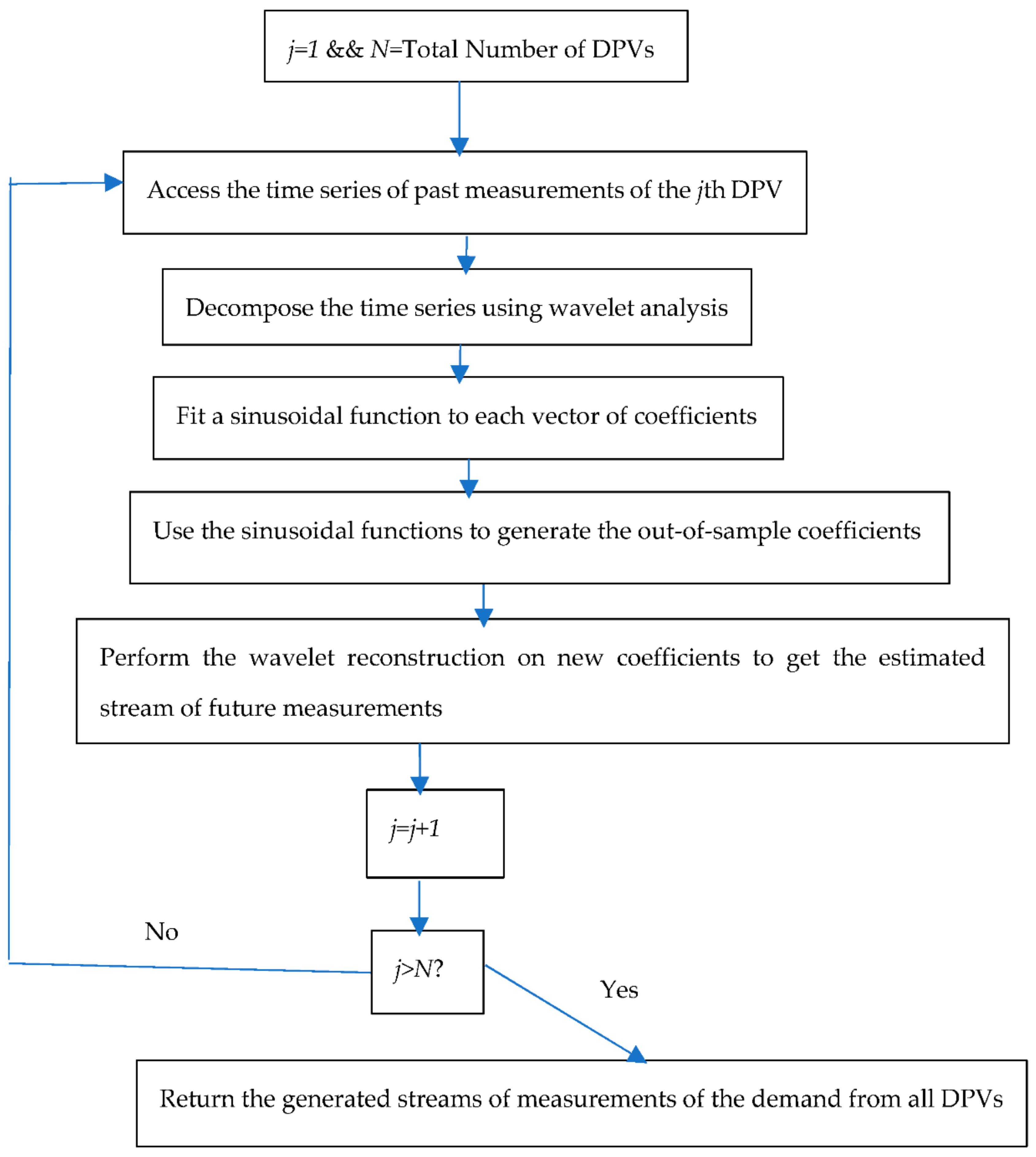
4.5. Data Generator
5. Results and Discussion
5.1. The Comparative Performance of PRDFS and BRDFS in Terms of Demand Forecasting Resilience to Stealth Attacks
Major Findings
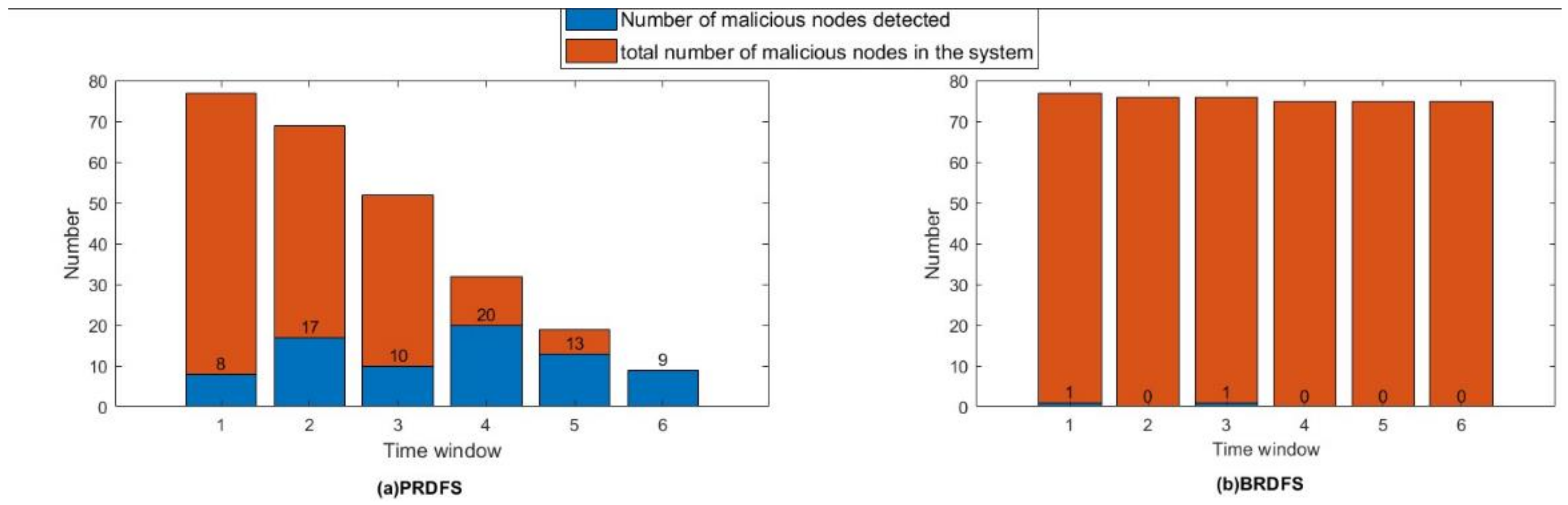
- PRDFS exhibits an almost perfect mean resilience value of over the time frame of the game (i.e., 1000-time steps) regardless of the percentage of the nodes compromised by the adversary (Figure 7). This is mainly because it detects and recovers all compromised nodes at the very early stages of games (within first 30-time steps) (Figure 10).

- During the first 40-time steps of games while the attack is still occurring or just ended, the mean demand forecasting resilience of PRDFS slightly decreases but it never goes below 0.8 (its resilience ranges from 0.82 to 1), regardless of the percentage of the malicious nodes (Figure 7). In contrast, the mean demand forecasting resilience sharply decreases in BRDFS over the simulation period (i.e., 1000 time-steps) as the percentage of malicious nodes increases (Figure 7).
- In PRDFS, the interval demand forecast accuracy demonstrates greater resilience than the point demand forecast accuracy, while the opposite trend is observed in BRDFS (Figure 7). In BRDFS, the interval demand forecast accuracy has weaker resilience compared to the point demand forecast accuracy and the trend becomes more pronounced as the percentage of malicious nodes increases. This is mainly because BRDFS fails to detect most malicious nodes (Figure 11). All colluding malicious nodes report similar measurements and thereby artificially reduce the uncertainty around the mean estimate, which results in low interval demand forecast accuracy and yields a very high FPR in detecting malicious nodes.
5.2. The Comparative Performance of PRDFS and BRDFS in Detecting Malicious Nodes
5.2.1. Major Findings:
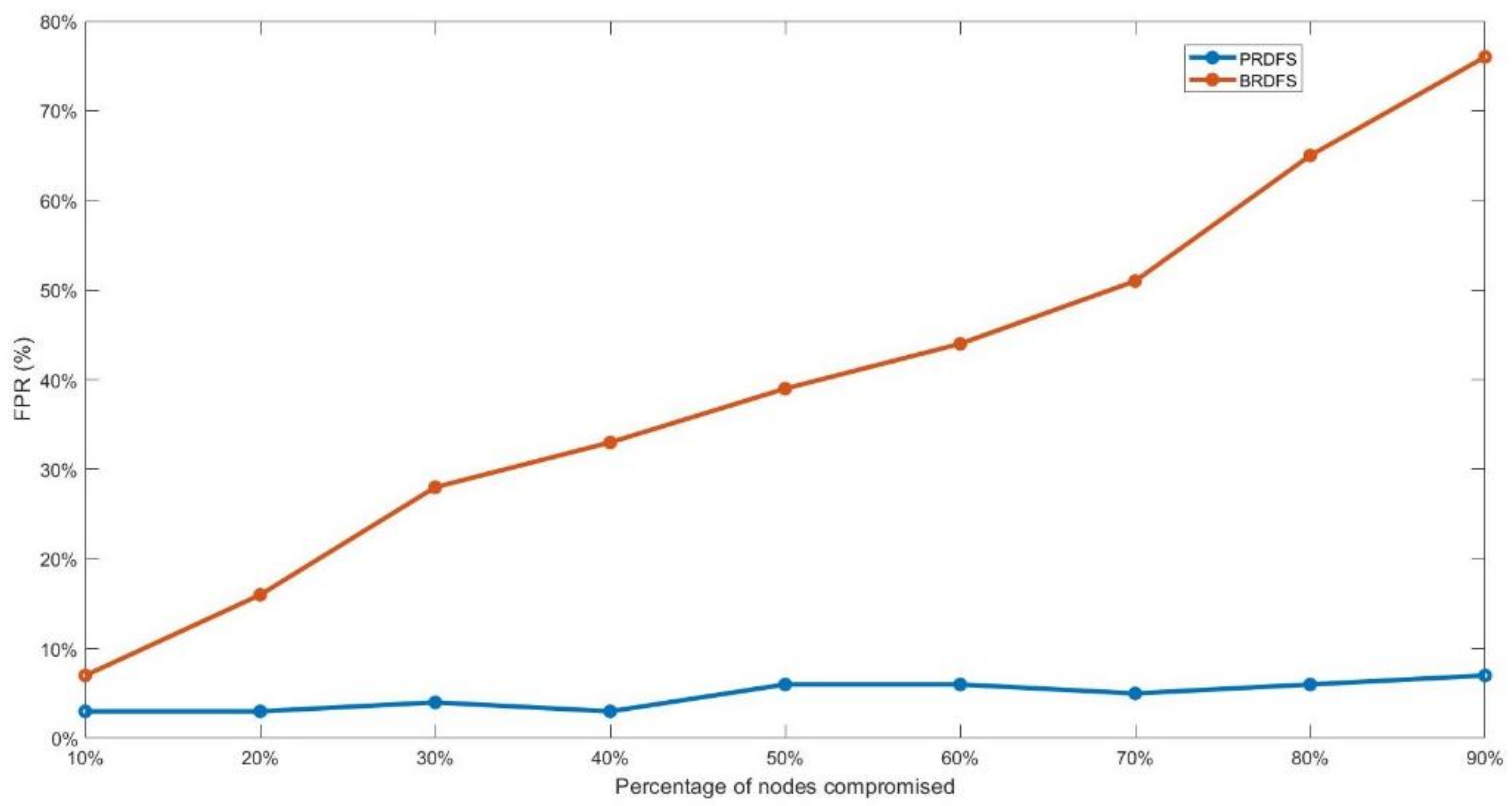
- PRDFS maintains a high malicious node detection accuracy of around 95% (ranging from 97% to 89%) while still maintaining a low FPR, ranging from 3–9%, with the increasing percentage of malicious nodes (Figure 8 and Figure 9). In contrast, the accuracy of BRDFS sharply falls with the rising FPR as the percentage of malicious nodes increases (Figure 8 and Figure 9).


- PRDFS successfully detects all malicious nodes within the first 30-time steps regardless of the percentage of the malicious nodes, whereas BRDFS fails to detect any malicious node after 15-time steps (Figure 10). It appears that BRDFS has a shorter time window for detecting malicious nodes than PRDFS.


5.2.2. Further Observations
- PRDFS uses a supervised intrusion detection system (SIDS) for detecting malicious nodes.
- ⮚
- SIDS learns from the input and output data sets that are contamination-free since they are generated through the game theoretic approach. It employs a supervised learning algorithm (GRNN) to distinguish between malicious and normal nodes.
- ⮚
- It can detect malicious nodes even when all nodes are malicious because it compares the present behaviors of the nodes in respect to dynamic spatio-temporal patterns of trustworthiness and the skewness of residual distribution with previous correct behaviors.
- BRDFS uses an unsupervised anomaly-based intrusion detection system (AIDS) for detecting malicious nodes.
- ⮚
- AIDS learn from unlabeled real data that are contaminated with many undetected malicious nodes. Hence, its learning is not very effective.
- ⮚
- AIDS learn under the assumption that statistically rare or atypical behaviors are abnormal and are possible signs of maliciousness, whereas typical or common behaviors are normal. Hence, AIDS can only detect malicious nodes when the percentage of malicious nodes is low, and the malicious nodes are operating for a short period of time where it is not possible to inject a significant number of malicious instances in the data set. However, stealthy malicious nodes are highly difficult to detect at very early stage.
- ⮚
- The skewness detector and the temporal collusion detection scheme of CAD uses confidence interval-based anomaly detection. If a node’s behavioral traits fall outside the confidence interval, the node is detected as malicious. However, such a strategy is ineffective against collusion attacks. In collusion attacks, the adversary takes control of multiple sensors and changes the readings of these sensors to the desired upward or downward direction in such a way that the malicious nodes always lie within the confidence intervals of correlation coefficients and skewness coefficients. One of the major challenges in time series forecasting is that the distribution of the time series changes over time. Hence, the forecasting model needs to be adapted to the most recent data—the adversaries take advantage of this situation. Returning the upper or lower extreme of the acceptable range as the readings of the compromised sensors, they can gradually move the forecasting model in the wrong direction without getting caught. Since the forecasting model is evolving towards the false data, over time, the non-compromised sensors are marked as compromised one after another and will lose all influence over the model’s evolution, thereby accelerating the compromise rate of the entire forecasting system.
- ⮚
- The spatial collusion detector of the CAD in BRDFS uses unsupervised clustering to separate malicious nodes. These clustering algorithms are based on arbitrary rules. Thus, it is natural that its accuracy is not as good as PRDFS.
5.3. The Comparative Performance of PRDFS and BRDFS in Estimating the Most Trustworthy Measurement of the Current Aggregate Demand
5.3.1. Major Findings
- Since PRDFS detects and recovers all compromised nodes at the very early stages of games (within first 30-time steps) (Figure 10), the mean accuracy of estimating in PRDFS is almost constant to around 98% over the time frame of the game (i.e., 1000-time steps) regardless of the percentage of the nodes compromised by the adversary (Figure 12).
- During the first 40-time steps of games, while the attack is still occurring or just ended, the mean estimation accuracy in PRDFS decreases from around 98% to 83% as the percentage of malicious nodes increases. In contrast, the mean estimation accuracy in BRDFS falls sharply over the simulation period (i.e., 1000 time-steps) as the percentage of malicious nodes increases.

5.3.2. Further Observations
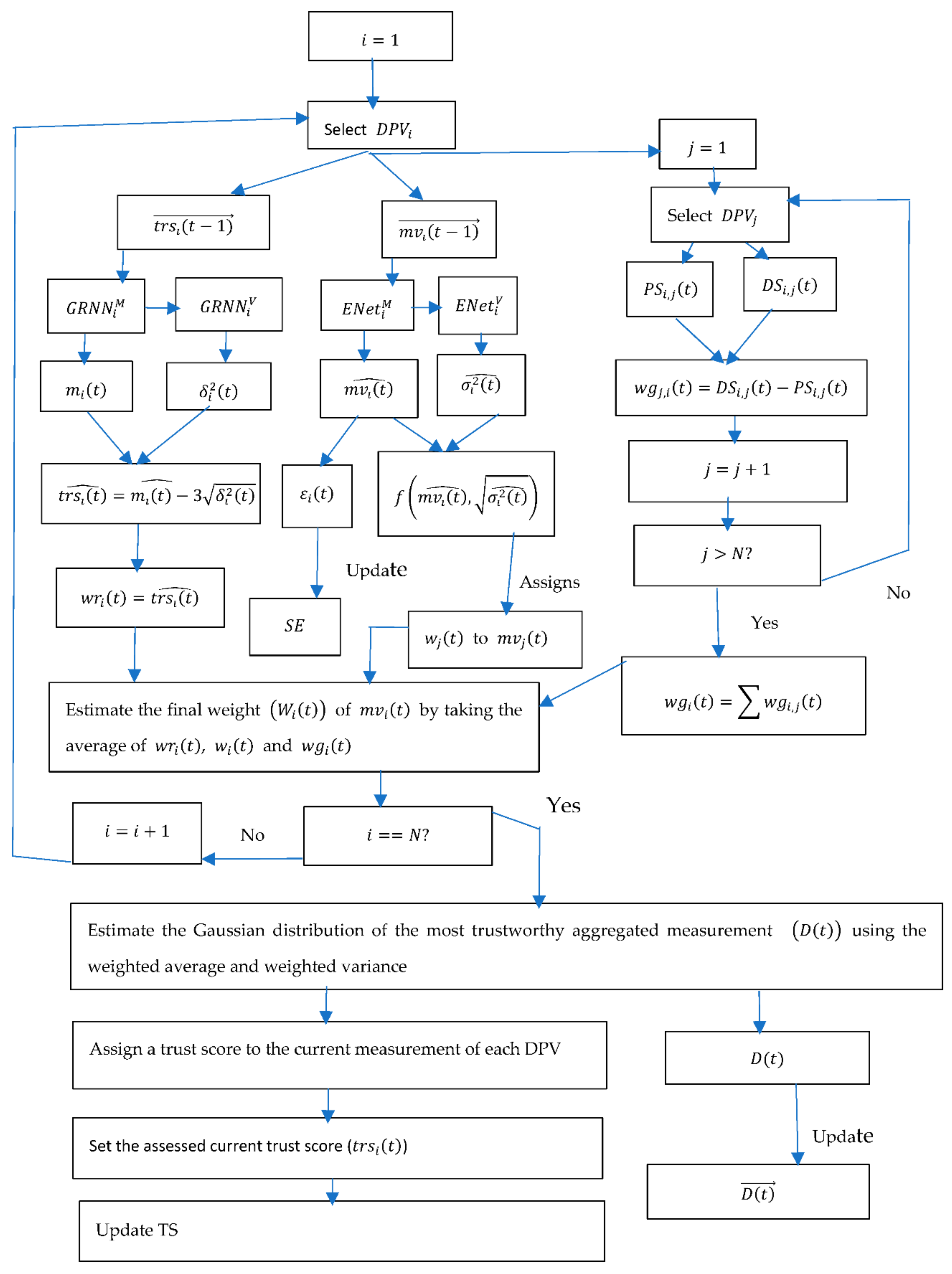
- The TMS of PRDFS considers the following three factors in determining the trustworthiness of a sensor node at a time distant : (1) the trustworthiness of the node, (2) the similarity of the sensor’s reading with the other sensors’ readings at the same time step, and (3) the similarity of the sensor’s measurement at time step with its past measurements, but in contrast, the TMS of BRDFS uses only the first two factors.
- The TMS of BRDFS updates the reputation score of a node at the end of a time step after determining the most trustworthy measurement at that time step. In the presence of on-off attacks, the normal behavior of a node at the last few time steps does not guarantee normal behavior from the node at the next time step. For this reason, the TMS of PRDFS predicts the trust score of a node at the beginning of a time step (before determining the most trustworthy measurement at that time step) using GRNN, which is a powerful pattern recognition algorithm capable of learning local patterns.
- In BRDFS, the reputation score of a node at time step is a linear function of its long-term reputation and its intermediate reputation score computed at time step . In contrast, the TMS of PRDFS uses a powerful fuzzy clustering-based non-linear algorithm (GRNN) to predict the trust score of a node at time step based on its past trustworthiness scores.
- The TMS of BRDFS sets the reputation score of a node at time step to the estimated expected (i.e., mean) reputation score of the node at time step . In stealthy on-off attacks, where at each time step the malicious nodes randomly choose whether to act maliciously or not, the variance of their reputation is an important indicator of their conditions. Hence, the point estimate of the expected reputation score is not very reliable. To overcome this problem, the TMS of PRDFS sets the trust score of a node to the lower bound of the predicted distribution of the plausible trust scores of the node at time step
5.4. The Comparative Performance of PRDFS and BRDFS in Terms of Demand Forecasting when No Attack Is Underway
5.4.1. Major Findings
- PRDFS outperforms BRDFS in terms of demand forecasting accuracy by 15% or more (Figure 13).

5.4.2. Possible Explanations
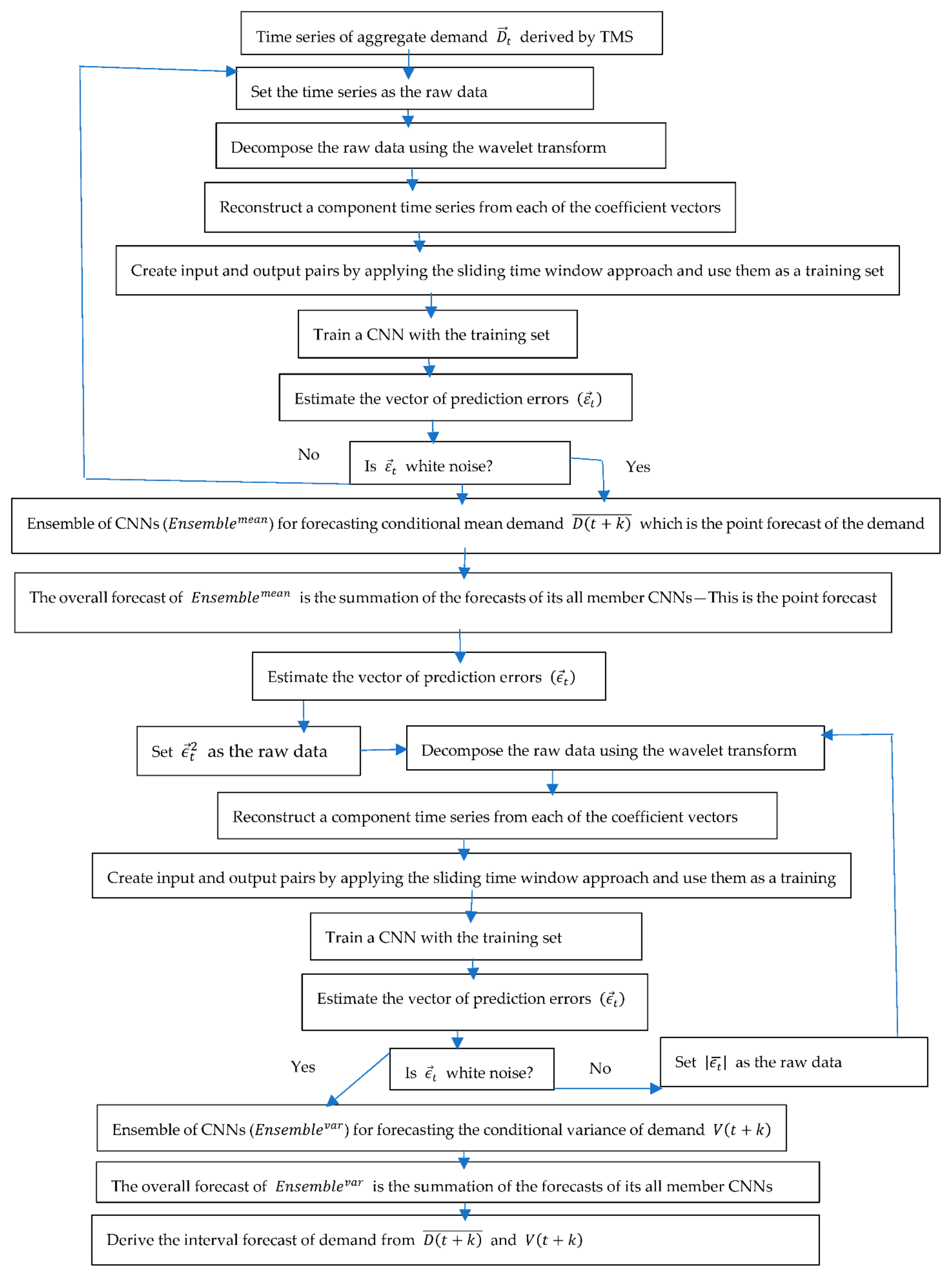
- The curse of dimensionality hits particularly hard on time series forecasting models of high or even moderate dimensional input data, since they use lagged variables as predictor variables and the lagged variables are highly correlated with each other. Hence, to reduce the dimensionality further, the DFS of PRDFS uses a hierarchical ensemble model where each member CNN is trained with only a small number of non-seasonal lagged variables. Ensemble members are trained sequentially. The first ensemble member is trained on the original demand time series. Each of the remaining ensemble members is trained on the residual series of the previous trained ensemble member. Additionally, the DFS of PRDFS uses CNNs as ensemble members. Our study suggests that CNN is more robust to the high dimensionality compared to other existing learning algorithms.
- The DFS of BRDFS does not have any such effective strategy to deal with non-stationarity and high dimensionality. It just uses a single LSTM regression network to forecast the demand.
6. Conclusions
Supplementary Materials
Author Contributions
Funding
Institutional Review Board Statement
Informed Consent Statement
Conflicts of Interest
References
- Gudova, I.A.; Frau, O. Critical infrastructure in the era of IOT and automation. In Proceedings of the International Scientific Conferences; “Strategies XXI”, Supple; Command and Staff Faculty: Bucharest, Romania, 2020. [Google Scholar]
- Muralidhar, N.; Muthiah, S.; Sharma, R.; Ramakrishnan, N. Multivariate long-term state forecasting in cyber-physical systems: A sequence to sequence approach. In Proceedings of the 2019 IEEE International Conference on Big Data, Los Angeles, CA, USA, 9–12 December 2019; pp. 543–552. [Google Scholar] [CrossRef]
- Chekola, E.G.; Ochoa, M.; Chattopadhyay, S. SCOPE: Secure compiling of PLC in cyber-physical systems. Int. J. Crit. Infrastruct. Prot. 2021, 33, 100431. [Google Scholar] [CrossRef]
- Rogers, R.; Apech, E.; Richardson, C.J. Resilience of the Internet of Things (IoT) from an information assurance (IA) perspective. In Proceedings of the 2016 10th International Conference on Software, Knowledge, Information Management & Applications (SKIMA), Chengdu, China, 15–17 December 2016. [Google Scholar] [CrossRef]
- Lee, J.; Bagheri, B. A cyber-physical systems architecture for industry 4.0-based manufacturing systems. Manuf. Lett. 2015, 3, 18–23. [Google Scholar] [CrossRef]
- Asshibani, Y.; Mahmoud, Q.H. Cyber physical systems security: Analysis, challenges and solutions. Comput. Secur. 2017, 68, 81–97. [Google Scholar]
- Sethi, P.; Sarangi, S. Internet of Things: Architectures, protocols, and applications. J. Electr. Comput. Eng. 2017, 2017, 9324035. [Google Scholar] [CrossRef]
- Ghalehkhondabi, I.; Ardjmand, E.; Young, W.A.; Weckman, G.R. Water demand forecasting: Review of soft computing methods. Environ. Monit. Assess. 2017, 189, 313. [Google Scholar] [CrossRef]
- Zhou, X.; Li, Y.; Barreto, C.A.; Li, J.; Volgyesi, P.; Neema, H.; Koutsoukos, X. Evaluating resilience of grid load predictions under stealthy adversarial attacks. In Proceedings of the 2019 Resilience Week (RWS), San Antonio, TX, USA, 4–7 November 2019; pp. 206–212. [Google Scholar] [CrossRef]
- Hoque, M.E.; Thavaneswaran, A.; Appadoo, S.S.; Thulasiram, R.K.; Banitalebi, B. A novel dynamic demand forecasting model for resilient supply chains using machine learning. In Proceedings of the 2021 IEEE 45th Annual Computers, Software, and Applications Conference (COMPSAC), Madrid, Spain, 12–16 July 2021. [Google Scholar] [CrossRef]
- Karthik, N.; Ananthanarayana, V.S. Data trustworthiness in wireless sensor networks. In Proceedings of the 2016 IEEE Trustcom/BigDataSE/ISPA, Tianjin, China, 23–26 August 2016. [Google Scholar] [CrossRef]
- Agarwal, V.; Pal, S.; Sharma, N.; Sethi, V. Identification of defective nodes in cyber-physical systems. In Proceedings of the 2020 IEEE 17th International Conference on Mobile Ad Hoc and Sensor Systems (MASS), Delhi, India, 10–13 December 2020. [Google Scholar] [CrossRef]
- El-Rewini, Z.; Sadatssharan, K.; Sugunaraj, N.; Selvaraj, D.F.; Plathottam, S.J.; Ranganathan, P. Cybersecurity attacks in vehicular sensors. IEEE Sens. J. 2020, 20, 13752–13767. [Google Scholar] [CrossRef]
- Jeba, S.V.; Paramasivan, B. Faalse data injection attack and its countermeasures in wireless sensor networks. Eur. J. Sci. Res. 2012, 82, 248–257. [Google Scholar]
- Tian, M.; Dong, Z.; Wang, X. Analysis of false data injection attackss in power systems: A dynamic Bayesian game-theoretic approach. ISA Transsactions 2021, 115, 108–123. [Google Scholar] [CrossRef]
- Kumari, A.; Tanwar, S. RAKSHAK: Resilient and scalable demand response management scheme for smart grid systems. In Proceedings of the 2021 11th International Conference on Cloud Computing, Data Science & Engineering (Confluence), Noida, India, 28–29 January 2021; pp. 309–314. [Google Scholar] [CrossRef]
- Barreto, C.; Koutsoukos, X. Design of load forecast systems resilient against cyber-attacks. In Decision and Game Theory for Security. Alpcan, T., Vorobeychik, Y., Baras, J., Dan, G., Eds.; Springer: Cham, Switzerland, 2019. [Google Scholar] [CrossRef]
- Babar, M.; Tariq, M.U.; Jan, M.A. Secure and resilient demand side management engine using machine learning for IoT-enabled smart grid. Sustain. Cities Soc. 2020, 62, 102370. [Google Scholar] [CrossRef]
- Chen, Q.; Zhang, C.; Zhang, S. Detection Models of Collusion Attacks. In Secure Transaction Protocol Analysis; Lecture Notes in Computer Science; Springer: Berlin/Heidelberg, Germany, 2008; Volume 5111. [Google Scholar] [CrossRef]
- Karthik, N.; Ananthanarayana, V.S. A hybrid trust management scheme for wireless sensor networks. Wirel. Pers. Commun. 2017, 97, 5137–5170. [Google Scholar] [CrossRef]
- Labraoui, N.; Gueroui, M.; Sekhri, L. On-off attacks mitigation against trust systems in wireless sensor networks. In Computer Science and Its Applications; Amine, A., Bellatreche, L., Elberrichi, Z., Neuhold, E., Wrembel, R., Eds.; IFIP Advances in Information and Communication Technology; Springer: Cham, Switzerland, 2015; Volume 456. [Google Scholar] [CrossRef]
- Lv, Z.; Han, Y.; Singh, A.K.; Manogaran, G.; Lv, H. Trustworthiness in industrial IoT systems based on artificial intelligence. IEEE Trans. Ind. Inform. 2021, 17, 1496–1504. [Google Scholar] [CrossRef]
- Hassan, S.; Khossravi, A.; Jaafar, J. Examining performance of aggregation algorithms for neural network-based electricity demand forecasting. Electr. Power Energy Syst. 2015, 64, 1098–1105. [Google Scholar] [CrossRef]
- Gheitasi, K.; Lucia, W. Undetectable Finite-Time Covert Attack on Constrained Cyber-Physical Systems. IEEE Trans. Control. Netw. Syst. 2022, 9, 1040–1048. [Google Scholar] [CrossRef]
- Ozer, O.; Zheng, Y. Trust and Trustworthiness. In The Handbook of Behavioral Operations, 1st ed.; Donohue, K., Katok, E., Leider, S., Eds.; Wiley Online Library: Hoboken, NJ, USA, 2018; pp. 489–523. [Google Scholar]
- Lopez, J.; Roman, R.; Agudo, I.; Fernandez-Gago, C. Trust management systems for wireless sensor networks:best practices. Comput. Commun. 2010, 33, 1086–1093. [Google Scholar] [CrossRef]
- Mohammadi, V.; Rahmani, A.M.; Darwesh, A.M.; Sahafi, A. Trust-based recommendation systems in internet of things: A systematic literature review. Hum.-Cenric Comput. Inf. Sci. 2019, 9, 21. [Google Scholar] [CrossRef]
- Ryutov, T.; Neuman, C. Trust based approach for improving data reliability in industrial sensor networks. In IFIP International Federation for Information Processing; Etalle, S., Marsh, S., Eds.; Springer: Boston, MA, USA, 2007; Volume 238, pp. 154–196. [Google Scholar] [CrossRef]
- Momani, M.; Challa, S.; Al-Hmouz, R. Bayesian fusion algorithm for inferring trust in wireless sensor networks. J. Netw. 2010, 5, 815–822. [Google Scholar] [CrossRef]
- Marinenkov, E.; Chuprov, S.; Viksnin, I.; Kim, I. Empirical study on trust, reputation, and game theory approach to secure communication in a group of unmanned vehicles. In Proceedings of the MICSECS, Saint Petersburg, Russia, 12–13 December 2019. [Google Scholar]
- Lim, H.-S.; Moon, Y.-S.; Bertino, E. Provenance-based trustworthiness assessment in sensor networks. In Proceedings of the Seventh International Workshop on Data Management for Sensor Networks, Singapore, 13 September 2010; pp. 2–7. [Google Scholar] [CrossRef]
- Lotufo, A.D.P.; Minussi, C.R. Electric power systems load forecasting: A survey. In Proceedings of the International Conference on Electric Power Engineering, Power Tech, Budapest, Budapest, Hungary, 29 August–2 September 1999. [Google Scholar] [CrossRef]
- Fallah, S.N.; Deo, R.C.; Shojafar, M.; Conti, M.; Shamshirband, S. Computational intelligence approaches for energy load forecasting in smart energy management grids: State of the art, future challenges, and research directions. Energies 2018, 11, 596. [Google Scholar] [CrossRef]
- Bose, J.-H.; Flunkert, V.; Gasthaus, J.; Januschowski, T.; Lange, D.; Salinas, D.; Schelter, S.; Seeger, M.; Wang, Y. Probabilistic demand forecasting at scale. Proc. VLDB Endow. 2017, 10, 1694–1705. [Google Scholar] [CrossRef]
- Salles, R.; Belloze, K.; Porto, F.; Gonzalez, P.H.; Ogasawara, E. Nonstationary time series transformation methods: An experimental review. Knowl.-Based Syst. 2019, 164, 274–291. [Google Scholar] [CrossRef]
- Panapakidis, I.P.; Dagoumas, A.S. Day-ahead natural gas demand forecasting based on the combination of wavelet transform and ANFIS/genetic algorithm/neural network model. Energy 2017, 118, 231–245. [Google Scholar] [CrossRef]
- Hu, Y.; Li, H.; Yang, H.; Sun, Y.; Sun, L.; Wang, Z. Detecting stealthy attacks against industrial control systems based on residual skewness analysis. EURASIP J. Wirel. Commun. Netw. 2019, 2019, 74. [Google Scholar] [CrossRef]
- Bhuiyan, M.Z.A.; Wu, J. Collussion attack detection in networked systems. In Proceedings of the 2016 IEEE 14th Intl Conf on Dependable, Automatic and Secure Computing, Aukland, New Zealand, 8–12 August 2016; pp. 286–293. [Google Scholar] [CrossRef]
- Albawi, S.; Mohammed, T.A.; Al-Zawi, S. Understanding of a convolutional neural network. In Proceedings of the 2017 International Conference on Engineering and Technology (ICET), Antalya, Turkey, 21–23 August 2017. [Google Scholar] [CrossRef]
- Specht, D.F. A general regression neural network. IEEE Trans. Neural Netw. 1991, 2, 568–576. [Google Scholar] [CrossRef] [PubMed]
- Zhang, D. Wavelet Transform. In Fundamentals of Image Data Mining; Texts in Computer Science; Springer: Cham, Switzerland, 2019. [Google Scholar] [CrossRef]
- Wang, D.; Tan, D.; Liu, L. Particle swarm optimization algorithm: An overview. Soft Comput. 2018, 22, 387–408. [Google Scholar] [CrossRef]
- Mishra, M.K.; Murari, K.; Parida, S.K. Demand-side management and its impact on utility and consumers through a game theoretic approach. Int. J. Electr. Power Energy Syst. 2022, 140, 107995. [Google Scholar] [CrossRef]
- Fu, W.; Chien, C-F. UNISON data-driven intermittent demand forecast framework to empower supply chain resilience and an empirical study in electronics distribution. Comput. Ind. Eng. 2019, 135, 940–949. [Google Scholar] [CrossRef]
- Kim, S.; Kim, H. A new metric of absolute percentage error for intermittent demand forecasts. Int. J. Forecast. 2016, 32, 669–679. [Google Scholar] [CrossRef]


| Term | Definition |
|---|---|
| Total number of DPVs | |
| Current time step | |
| Data provenance of the ith measurement | |
| Data provenance of the jth measurement | |
| The total number of nodes common to and | |
| The lenght of the longer DPV between and | |
| Time series of the ith DPV’s measurements containing both past and current measurements | |
| Time series of the ith DPV’s past measurements | |
| The received measurement of the ith DPV at time step t | |
| The received measurement of the jth DPV at time step t | |
| The data similarity between and estimated using MAAPE | |
| Provenance similarity between the DPVs of and | |
| One step ahead forecast of the conditional mean of | |
| The residual series for the one step ahead forecasts of ith DPVs measurements containing both the past and current residuals | |
| The residual series for the one step ahead forecasts of ith DPVs measurements containing the past residuals | |
| The observed conditional variance of | |
| One step ahead forecast of | |
| The ensemble of CNNs forecasting | |
| The ensemble of CNNs forecasting based on | |
| A gaussian distribution with mean and standard deviation | |
| A matrix containing the residual series for the one step ahead forecasts of all DPVs measurements | |
| A matrix containing the time series of skewness of the series in | |
| The measurements of all DPVs at | |
| The most trustworthy aggregate demand measurement at time step based on | |
| The time series of aggregate demand | |
| Time series of the assessed trust scores of the ith DPV including its assessed trust score at time step t | |
| Time series of the assessed trust scores of the ith DPV, not including its assessed trust score at time step t | |
| The assessed trust score of the ith DPV at time step t | |
| The forecasted trust score of the ith sensor at time step t | |
| The forecasted conditional mean of based on | |
| The forecasted conditional variance of | |
| The ith member of GRNN of the ensemble of GRNNs forecasting | |
| The ith member of GRNN of the ensemble of GRNNs forecasting | |
| The most trustworthy aggregate demand measurement at time step t | |
| The time series of aggregate demand (based on ) including | |
| The k-step-ahead forecasted conditional mean aggregate demand based on | |
| The k-step-ahead forecasted value of the conditional variance of | |
| The ensemble of CNNs forecasting | |
| The ensemble of CNNs forecasting | |
| Measurement generated for the ith DPV at time step t by DG | |
| contains the measurements generated by DG for all sensors at t: | |
| The most trustworthy aggregate demand measurement at time step t based on | |
| The time series of aggregate demand (based on ) including | |
| The k-step-ahead forecasted conditional mean aggregate demand based on | |
| The position of the qth particle at time step t and iteration I. | |
| The most trustworthy aggregate demand measurement at time step t based on | |
| The time series of aggregate demand (based on ) including | |
| The k-step-ahead forecasted conditional mean aggregate demand based on | |
| is the velocity of the qth particle. | |
| The fitness score of | |
| The personal best position of the qth particle | |
| The fitness score of | |
| The global best position of all the particles | |
| The fitness score of | |
| is a matrix containing the time series of the states (malicious and normal) of each sensor at previous time steps | |
| A vector containing the state of each DPV in the qth particle at time step t and iteration I | |
| A vector containing the state of each DPV at the beginning of a game | |
| A vector containing the state of each DPV in |
| Predicted Label | |||
|---|---|---|---|
| Positive (Malicious) | Negative (Normal) | ||
| Actual Status | Positive (Malicious) | True Positive (TP) | False Negative (FN) |
| Negative (Normal) | False Positive (FP) | True Negative (TN) | |
Publisher’s Note: MDPI stays neutral with regard to jurisdictional claims in published maps and institutional affiliations. |
© 2022 by the authors. Licensee MDPI, Basel, Switzerland. This article is an open access article distributed under the terms and conditions of the Creative Commons Attribution (CC BY) license (https://creativecommons.org/licenses/by/4.0/).
Share and Cite
Gheyas, I.; Epiphaniou, G.; Maple, C.; Lakshminarayana, S. A Resilient Cyber-Physical Demand Forecasting System for Critical Infrastructures against Stealthy False Data Injection Attacks. Appl. Sci. 2022, 12, 10093. https://doi.org/10.3390/app121910093
Gheyas I, Epiphaniou G, Maple C, Lakshminarayana S. A Resilient Cyber-Physical Demand Forecasting System for Critical Infrastructures against Stealthy False Data Injection Attacks. Applied Sciences. 2022; 12(19):10093. https://doi.org/10.3390/app121910093
Chicago/Turabian StyleGheyas, Iffat, Gregory Epiphaniou, Carsten Maple, and Subhash Lakshminarayana. 2022. "A Resilient Cyber-Physical Demand Forecasting System for Critical Infrastructures against Stealthy False Data Injection Attacks" Applied Sciences 12, no. 19: 10093. https://doi.org/10.3390/app121910093
APA StyleGheyas, I., Epiphaniou, G., Maple, C., & Lakshminarayana, S. (2022). A Resilient Cyber-Physical Demand Forecasting System for Critical Infrastructures against Stealthy False Data Injection Attacks. Applied Sciences, 12(19), 10093. https://doi.org/10.3390/app121910093