1. Introduction
Deep learning methods have yielded significant success in several complicated applications, such as image classification [
1,
2,
3] and object detection [
4,
5,
6,
7]. It is essential to train a deep convolutional neural network with an excellent optimizer to obtain considerable accuracy and convergence speed. Stochastic gradient descent (SGD) [
8] is one of the primary and dominant optimizers that performs well across many applications due to its simplicity [
9,
10]. However, SGD scales the gradients uniformly in all directions with a constant learning rate. This strategy leads to a slow training process and sensitivity to tuning learning rates. Recent works proposed various adaptive gradient methods to achieve faster convergence by computing individual learning rates for different gradients to address this problem. Examples of these adaptive methods include AdaGrad [
11], RMSProp [
12], and Adam [
13]. These methods use the exponential moving average (EMA) [
14] of the past square gradients to adjust the learning rates. Particularly, Adam is one of the famous adaptive gradient methods, and it has become the alternative optimizer after SGD(M) across many deep learning frameworks because of its rapid training speed [
15,
16]. Despite their popularity, there is still a performance gap between the adaptive gradient methods with well-tuned SGD (M) [
17].
However, recent theories have shown that Adam suffers from non-convergence issues and weak generalization [
15,
18]. An empirical study showed that the parameters of Adam update unstably; its second moment could be out of date, resulting in producing inappropriate learning rates based on the changes in gradients [
19]. The second moment of Adam in training has been found to produce extreme learning rates; the extreme or abnormal learning rates encountered during training cause poor generalization performance of Adaptive methods [
20].
Reddi et al. [
18] proposed a variant of Adam called AMSGrad to solve the shortcomings of Adam as mentioned above. Although the authors provide a theoretical guarantee of convergence, AMSGrad only shows better results on training data. However, a study further indicated that AMSGrad does not show noticeable improvement over Adam [
21].
Another work to fix the problems of Adam is called AdaBound [
20]. AdaBound borrows the truncating theory of gradient clipping [
22] to constrain the unreasonable learning rates of Adam by two hand-designed asymptotical functions: the upper bound function
and the lower bound function
. These two functions tend to a constant value that transforms Adam to SGD (M) gradually. The experiments in [
20] demonstrate that AdaBound maintains a rapid training speed, like Adam, in the early and achieves a considerable generalization, like SGD (M), in the end. Additionally, the parameters of bound functions are not sensitive and default parameters are recommended for all classification tasks. In contrast, the experiments reported in [
23] showed that AdaBound does not outperform Adam and others, the poor performance of AdaBound could be caused by the default parameters because the same bound are recommended for all classification task. Savarese [
24] showed that the bound functions strongly affect the optimizer’s behavior and might require careful tuning.
A reasonable learning rate range refers to the reasonable learning rates that a current task can converge, the maximum value of this range is considered the largest learning rate that does not cause the disconvergence of training criteria [
25]. However, AdaBound is empirically hand-designed for its bounds, which are independent of tasks. So, it remains a problem to AdaBound that its bounds are able to accurately and completely truncate the unreasonable learning rates or not during training, because the unreasonable learning rates of a certain task are not stated explicitly. Therefore, it is imperative to specify the reasonable convergence range of Adam for a certain task to accurately distinguish the unreasonable learning rates, and design the bound functions according to reasonable convergence range to achieve a smooth transformation from Adam to SGD (M) without any unreasonable learning rates.
To address the problem of AdaBound, we proposed a new variant of the adaptive gradient descent method with a convergence range bound, which is called AdaCB. The major contributions of this paper are summarized as follows:
The LR range test [
26] is used to accurately determine the reasonable convergence learning rate range for Adam instead of empirically hand designed, which can distinguish the unreasonable learning rates for a certain task.
Inspired by the clipping method, the learning rates of Adam are constrained by two asymptotical functions: upper bound and lower bound. The upper bound is the asymptotical function that starts from the maximum value of the convergence range and gradually approaches the global fixed learning rate. The lower bound is the asymptotical function that starts from 0, and gradually approaches the global fixed learning rate.
We evaluate our proposed algorithm for the image classification task. Smallnet [
27], Network IN Network [
28], and Resnet [
29] are trained on CIFAR10 [
30] and CIFAR100 [
30] datasets. Experiment results show that our proposed method behaves like an adaptive gradient method with a faster convergence speed, and achieves considerable results like SGD (M).
The rest of our paper is organized as follows. In
Section 2, we review the background of traditional optimizers and adaptive gradient optimizers. In
Section 3, we introduce our proposed AdaCB. In
Section 4, we conduct experiments to verify the effectiveness of our method. In
Section 5, we discuss the advantages and disadvantages of our proposed optimizer. In
Section 6, we summarize the paper.
2. Related Works
Training neural networks are about tuning the weights with the lowest loss function by learning algorithms (gradient descent methods) to produce an accurate model for classification or prediction [
31]. In general, there are two types of gradient descent methods: stochastic gradient descent methods and adaptive gradient descent methods.
2.1. Stochastic Gradient Descent (SGD)
SGD is the primary and dominant algorithm for CNN models. The SGD updates the weights with a constant learning rate, which is shown in the following Equation (1). The stands for weights at the step and stands for the updated weights after that step . The denotes the gradients for corresponding weights at the step and stands for the global learning rate, which is often set from 0.1, 0.01, and 0.001. SGD takes a long time for training and is sensitive to learning rates. For the sake of clarifying, the variables of , , , and stand for updated weights, current weights, current gradients, and current step respectively for the rest of the equations.
The general updating rule for weights in SGD:
2.2. SGD with Momentum
Inspired by the idea of momentum in physics, Poyak et al. [
32] proposed a variant of SGD called SGD with momentum, shortly named SGD (M). The cumulative momentum speed
is introduced to affect the updating direction and
denotes the last corresponding indicator. The basic idea is that the direction and magnitude of the previous gradients contribute to the step size in the current step. As a result, the training speed is slightly improved.
The general updating rule for weights in SGD (M):
Calculating the cumulative momentum speed:
In Equations (2) and (3), the is the momentum term that determines the influence of previous gradients on the current update, which is set as close to 1 as possible. The is a global learning rate like vanilla SGD.
2.3. AdaGrad
However, SGDs scale the gradients in all directions with a constant learning rate, ignoring the sight of the difference between each parameter is not ideal. Therefore, the adaptive gradient descent methods are proposed. In such a situation, the parameter with the critical update should take a more significant step in the gradient direction than the parameter with a less critical update. In other words: to speed up the learning process, every parameter to be updated should have its learning rate in every step.
The first try is AdaGrad. This method calculates the individual learning rates for different parameters, given by a constant value dividing the root of the sum of the square of the past gradients from step 0 to . The updating rule is defined as following Equation (4).
The general updating rule for weights in AdaGrad:
where the
is a constant value, which is given by 0.001 in practice, and epsilon
is 1 × 10
−8 to avoid the zero of the denominator. The adaptive learning rates are determined by
. However, the denominator is the sum of squared gradients, which can lead to a monotonic increase. Therefore, the learning rates decrease monotonically, leading to slow updating or non-updating circumstances.
2.4. RMSProp
To address the problem of AdaGrad, RMSProp is developed. Instead, RMSProp uses an exponential moving average of square gradients, which is donated to , and is the last corresponding indicator. As a result, the denominator is not monotony increasing. Equations (5) and (6) show the updating rules. The momentum term of EMA is given by 0.9. The constant value is 0.001 in practice, and the epsilon is 1 × 10⁻⁸ to avoid the zero of the denominator.
The general updating rule for weights in RMSProp:
Calculating the EMA indicator of square gradients:
2.5. Adam
The Adaptive Moment Estimation (Adam) algorithm is another adaptive gradient method proposed by Kingma [
13], which is widely used in CNNs [
33]. It is an extension of RMSprop. Like RMSprop, an Exponential Moving Average of squared gradients
is used, and
stands as the last corresponding indicator. Additionally, an Exponential Moving Average of gradients
is included, and
is the last corresponding indicator. This new value resembles the average direction of the gradients to avoid non-updating cases caused by zero value of gradient. The authors also employ two bias corrections for these two EMA indicators, which are denoted as
and
. As a result, they could obtain proper estimations for both denominator and gradients in the early training stage. The formal notations are shown as follows Equations (7) to (11). The variables of
and
, which determine the memory time of that two EMA indicators. The authors suggest standard values of
for 0.9, and
for 0.999. The value of
is set as 0.001 in practice, and
is 1 × 10
−8.
The general updating rule for weights in Adam:
Calculating the EMA indicator of gradients:
Calculating the bias correction for EMA indicator of gradient:
Calculating the EMA indicator of square gradients:
Calculating the bias correction for EMA indicator of square gradient:
2.6. AMSGrad
In the recent paper “On the convergence of Adam and beyond” [
18], the authors indicated that Adam might suffer from non-convergence issues. Long-term memory should be emphasized to reduce the influence of non-informative gradients and eliminate unreasonable large learning rates. Therefore, the AMSGrad is proposed.
The AMSGrad differs at two points from the Adam algorithm. The first difference is that the AMSGrad only uses the EMA indicator of gradients and EMA predictor of square gradients , and omits the bias corrections for both and . Note that and are the last corresponding EMA indicators. The second difference concerning Adam is that the denominator calculation is replaced by taking the maximum value between the last indicator and the current indicator . In this way, a sort of long-term memory is incorporated into large gradients, which results in a non-increasing step size and avoids the pitfalls of Adam. However, the denominator increases monotonically because only the biggest variable is concerned, leading the slow updating or non-updating circumstances like AdaGrad. The formal notations of AMSGrad are described as follows Equations (12) to (15). The parameter setting is the same as Adam, where is 0.001, is 0.9, and is 0.999. The epsilon is 1 × 10⁻⁸.
The general updating rule for weights in AMSGrad:
Calculating the EMA indicator of gradients:
Calculating the EMA indicator of square gradients:
Taking the maximum operation for the denominator:
2.7. AdaBound
AMSGrad designed a strategy of non-increasing learning rates to tackle extreme learning rate problems. However, recent work has pointed out AMSGrad does not show evident improvement over Adam [
21]. Luo et al. [
20] speculate that Adam’s extremely large and small learning rates are likely to account for weak generalization ability. To this end, they proposed AdaBound which implemented a gradual transformation from Adam to SGD (M) by employing dynamic bounds to clip extreme ones. However, AdaBound only tackles the extreme learning rates at the end. AdaBound is described in the following Equations (16) to (23).
The general updating rule for weights in AdaBound:
Calculating the EMA indicator of gradients:
Calculating the bias correction for EMA indicator of gradient:
Calculating the EMA predictor of square gradient:
Calculating the bias correction for EMA predictor of square gradient:
Setting the lower bound function for Adam:
Setting the upper bound function for Adam:
Constraining the learning rates of Adam in these two bounds:
where the
is the lower bound and
is the upper bound, and
is considered as a global constant learning rate to the end. The value
controls the transition speed from Adam to SGD (M). The authors do the grid search on these two parameters, and they are not sensitive to accuracy. The
and the
are given to 0.999 and 0.1 for all tasks, respectively. The rest of the parameters are the same as Adam, which mention in the last
Section 2.5. In this setting, the bound range is empirically hand-designed without data information, which is an exhausting way. As a result, it is unknown whether bounds of AdaBound can properly truncate the unreasonable learning rates, because the unreasonable learning rates of a certain task are not state clearly. Intuitively, AdaBound uses the same bounds for all tasks because parameters are not sensitive, which may hurt the generalization performance of the algorithm [
23].
2.8. Differences and Similarities between Algorithms
The algorithms described above are considered the adaptive version of SGD because some terms or techniques are mutually used. The general updating rules of them can be described in the following Equation (24).
Most algorithms can be described as a uniquely used combination of a small number of building blocks in Equations (25) to (28), and they vary in some terms, as shown in
Table 1.
Calculating the EMA indicator of gradient:
Calculating the EMA indicator of square gradient:
Calculating the bias correction for EMA indicator of gradient:
Calculating the bias correction for EMA indicator of square gradient:
3. Proposed Algorithm
Inspired by Adam and Adabound, we propose a new optimizer with convergence range-bound named AdaCB. Firstly, the convergence range of Adam for a particular task is specified by the learning rate range test (LR test). Secondly, two bound functions named upper bound and lower bound are designed to clip the learning rates of Adam in this convergence range. The upper bound starts from the maximum value of the convergence range and approaches the global fixed learning rate asymptotically; the lower bound starts from zero value and approaches the global fixed learning rate asymptotically. In this setting, AdaCB behaves like Adam in the early stage and gradually transforms to SGD in the end, thus, extreme learning rates are considered during the whole stage because the bounds are specified.
3.1. Specify the Convergence Range for Adam
LR test is a helpful way to determine the reasonable convergence range of learning rate for a new model or dataset. LR test wraps the update part of an optimizer to train a model for several epochs and makes the learning rate gradually increase from small to large ones, then the acceptable range learning rate can be approximately estimated by the curve of the loss function. When the loss keeps decreasing, it means the current learning rate is acceptable, when the loss starts rising, it means the current learning rate is the proper largest learning rate the model can be converged.
Adam automatically adjusts the learning rates for different parameters by the formula
, which is always changed during training. We wrap the update part of Adam into the LR test as an individual value and make the value increase from small to large. When the loss starts rising, this current learning rate can be considered the maximum learning rate at which the model can be converged. The global fixed learning rate can be considered as the proper learning rate that the model can be converged stably. A global fixed learning rate is recommended as the common SGD (M) learning rate in which one order lower than the learning rate where loss is minimum [
26].
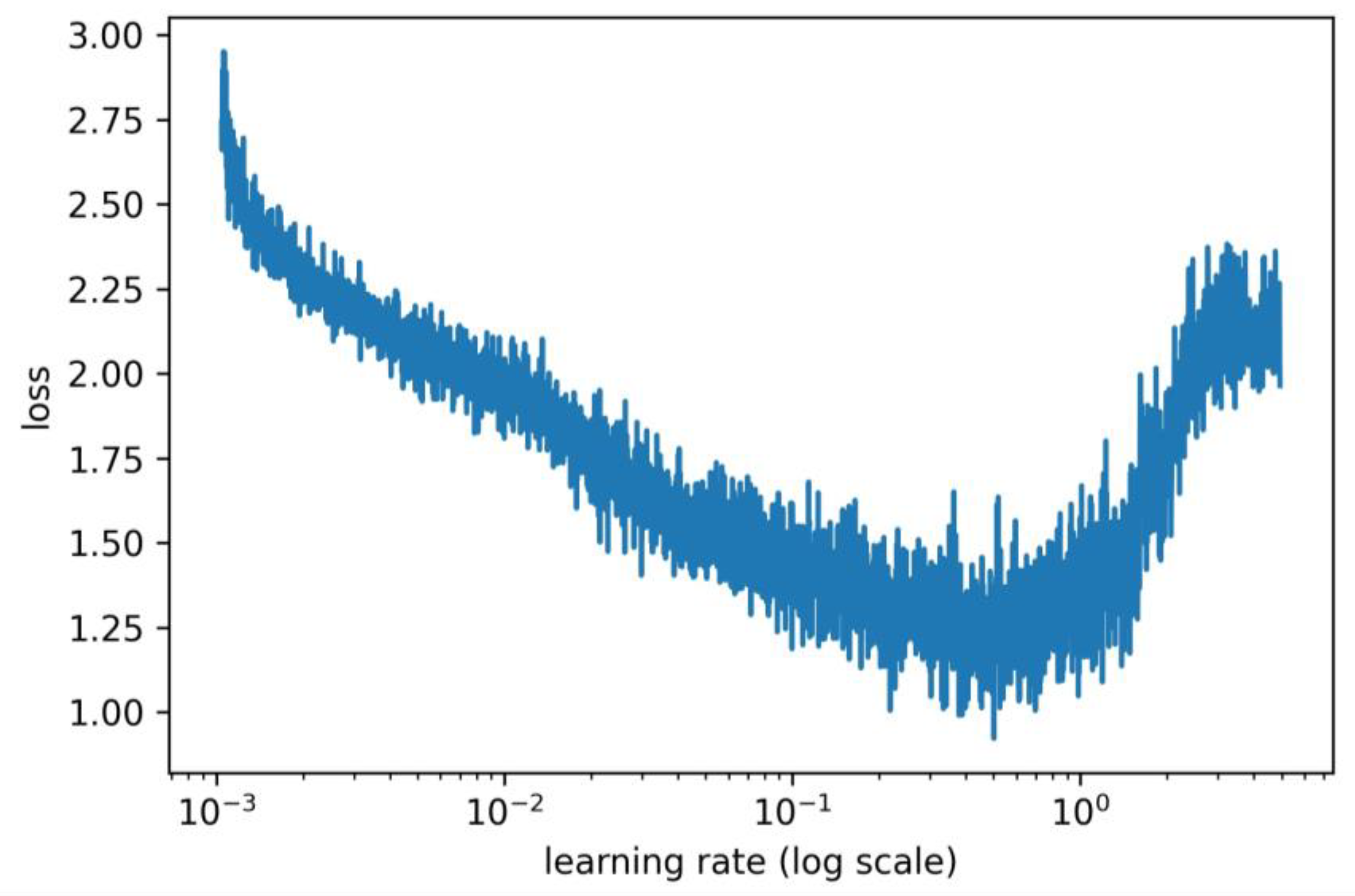
For example, we use the Smallnet [
27] architecture to perform the LR test wrapped with Adam on the CIFAR10 dataset [
30] and generate the curve of the loss function, which is shown in the following
Figure 1. As we can see in
Figure 1, the loss starts increasing when the current learning is approximately 0.5, so 0.5 is considered the maximum value that this particular task can be converged. The SGD (M) learning rate is commonly chosen from {0.1, 0.01, 0.001} [
34,
35], according to principle of choosing a global fixed learning rate [
26], the global fixed value can be 0.01.
3.2. Design the Bound Functions
Similar to AdaBound, the clipping operation
is employed on a reasonable learning rate range of Adam obtained by the above
Section 3.1, which can be demonstrated in the following Equation (29).
is donated as the learning rates of Adam,
is the lower bound function that starts from 0 to and gradually approaches the global fixed learning rate, and
is the upper bound function that starts from the maximum value of convergence range to the global fixed learning rate.
Clipping the learning rates of Adam in convergence range:
3.2.1. The Design of Upper Bound
The linear and exponential properties are the common and widely used mechanisms to solve some mathematical problems in practical [
36,
37,
38,
39,
40]. To tackle the extreme learning rates of Adam during whole training and achieve a smooth transformation from Adam to SGD, the upper bound is designed to be an asymptotical function from the maximum value of convergence range to the global fixed value. In this section, we define the two toy functions for the upper bound
, which can be linear and exponential according to basic math definitions [
41]. The upper bound functions are shown in the following Equations (30) and (31).
Linear asymptotic of upper bound:
Exponential asymptotic of upper bound:
where the
is the largest learning rate that a task can be converged, the
is the global fixed learning rate that a task can be converged stably, the
is the total training step of a particular task, and
is the current step,
is the certain moment that Adam completely transforms to SGD, and
is the clipping operation to take the minimum value 1 to avoid the range explosion. For the explanation of
, when the
is defined as 0.5, it takes 50 percent of training time to complete the asymptotical process from the largest learning rate to the global fixed learning rate. By this design principle, the upper bound can start from the largest learning rate of the convergence range and gradually approach the fixed learning rate at a certain moment, then
.
3.2.2. The Design of Lower Bound
For the lower bound, we design an asymptotical function that starts from zero and gradually approaches the upper bound. However, the upper bound gradually approaches a global fixed value, so the lower bound gradually approaches a global fixed value too. As a result, the lower bound depends on the upper bound, which varies for a particular task that enhances the flexibility of the range. Regarding the exponential design principle [
41], the initial value and denominator cannot be zero. Therefore, in this section, we only define the linear function for the lower bound
, which is shown in Equation (32).
Linear asymptotic of lower bound:
where
is the current training step and
is the total training step,
is the moment that Adam completely transforms to SGD (M), and
is the clipping operation to take the minimum value 1 to avoid the range explosion. By this design principle, the lower bound can start from zero value and gradually approach a global fixed value at a certain moment, then
.
3.3. Algorithm Overview for AdaCB
Based on the above analysis, this subsection demonstrates our proposed algorithm named AdaCB, which considers tackling the extreme learning rates during the whole training stage using specified bounds. The details of AdaCB are illustrated in Algorithm 1. The
and
can be found by the LR test mentioned in the last
Section 3.1. The
is the total training step, which is automatically calculated by
. The
is a certain moment when Adam completely transforms into SGD (M). For example, if we set it
, it takes 50 percent of the total training time to complete the transformation between Adam and SGD (M). The
,
and
are initial parameters of Adam. The
is the constraint operation in a range and the
and
are bound functions designed in the last
Section 3.2.1 and
Section 3.2.2.
In this setting, the AdaCB behaves like Adam in the early stage, and it gradually becomes SGD (M) in the end as two bounds tend to a fixed value. Additionally, the extreme learning rates are tackled during whole training because the bound ranges are specified particularly.
| Algorithm 1 AdaCB |
| Parameters: (parameters of our proposed algorithm) |
| Initialize: (initial parameters for Adam) |
| 1:set |
| 2:for do |
| 3: (calculating the gradients) |
| 4: (calculating EMA indicator of gradients) |
| 5: (calculating bias correction of EMA indicator of gradients) |
| 6: (calculating EMA indicator of square gradients) |
| 7: (calculating bias correction of EMA indicator of square gradients) |
| 6: (clipping the learning rates in the convergence range) |
| 8: (updating the weights) |
| 9:ends for |
4. Experiments
In this section, we validate our optimizer AdaCB on the image classification task and compare it to the other three state-of-the-art optimizers, including SGD (M), Adam, and AdaBound. The details of the optimizers are presented in previous
Section 2. All the experiments are implemented using Keras with the backend support of Tensorflow, while GeForce GTX 1060 6 GB GPU is utilized to accelerate the computations. Three CNN architectures with various depths and widths are used respectively to train on CIFAR10 and CIFAR100 datasets in a total of 100 epochs, which include Smallnet [
27], Network IN Network [
28], and 18 layers of Resnet [
29]. The batch size is set to 128. We report the average accuracy over five runs for each optimizer across different CNN architectures and datasets.
Data augmentation is a popular regularization technique used to expand the dataset size. However, it is difficult to isolate the impact of the data augmentation from the methodology [
42,
43]. To exclude complex data expansion that affected the final results, we only divide the original images by 255, and no data augmentation is used. Please note that we are only testing the performance of the optimizers, and we are not testing the effect of the regularization technique.
4.1. Hyper Parameter Tuning
The setting of hyper parameters has a great impact on the performance of the optimization algorithm. Here we describe how we adjust them. We follow Luo et.al. [
20] and implement a logarithmical grid search on a large space of learning rate for SGD (M) and take the best results. We set the recommended parameters for another adaptive gradient method. The hyper parameters of each algorithm are adjusted and summarized as follows:
SGD (M): we roughly tune the learning rate for SGD (M) on a logarithmic scale from {10, 1, 0.1, 0.01, 0.001} and then fine-tune it. We set the momentum parameter to the default value of 0.9. As a result, we set the learning rate of SGD (M) as 0.01 for CIFAR10 and CIFAR100 under Smallnet, Network IN Network, respectively; and 0.1 as the learning rate for CIFAR10 and CIFAR100 under Resnet18.
Adam: we set the recommended parameters for Adam, where , , .
AdaBound: we set the recommended parameters for AdaBound, where , , , , and .
AdaCB: We use the same hyper parameter settings for Adam. The
and
are determined by the LR test, which is mentioned in
Section 3.1. As a result, we set the
and the
on CIFAR10 and CIFAR100 under Smallnet; we set the
and
on CIFAR10 and CIFAR100 under Network IN Network; we set the
and
on CIFAR10 and CIFAR100 under Resnet18. The total training step is
. For more, we will conduct an empirical study to obtain the proper value for transformation speed and asymptotical behavior of the bound function.
4.2. Empirical Study on Behaviors of Bound Function and Transformation Speed
In the previous
Section 3.2.1, we propose a linear and exponential asymptotic function for the upper bound and a parameter for transformation speed. To investigate the proper behaviors of bound function and transformation speed
, we conduct a quick analysis with the Smallnet on CIFAR10 dataset, in which the moment
is chosen in {0.1, 0.2, 0.3, 0.4, 0.5, 0.6, 0.7, 0.8, 0.9, 1}. The results are shown in
Table 2. The experiment results show that linear behavior is better than exponential behavior intuitively, and the best result is obtained when
. For the sake of clarifying, we use linear behavior for the upper bound function and
in the rest of the experiments.
4.3. Results of Smallnet on CIFAR10 and CIFAR100
Figure 2 and
Figure 3 show the learning curve of testing accuracy for each gradient descent method on CIFAR10 and CIFAR100 under Smallnet architecture. We find that Adam has a faster convergence speed in the early stage, but it finally produces the worst test accuracy. Despite of slow convergence speed for SGD (M) in the early stage, SGD (M) gradually outperforms Adam and AdaBound with increasing training steps. AdaBound has a comparable convergence speed with SGD (M), but the testing accuracy is worse than SGD (M). Our proposed algorithm has a comparable convergence speed with Adam, and it achieves the highest testing accuracy. The detail of testing accuracy for each optimizer on CIFAR10 and CIFAR100 under Smallnet architecture is shown in
Table 3. According to
Table 3, AdaCB achieves the best accuracy over five runs, followed by SGD (M), AdaBound, and Adam.
4.4. Results of Network in Network on CIFAR10 and CIFAR100
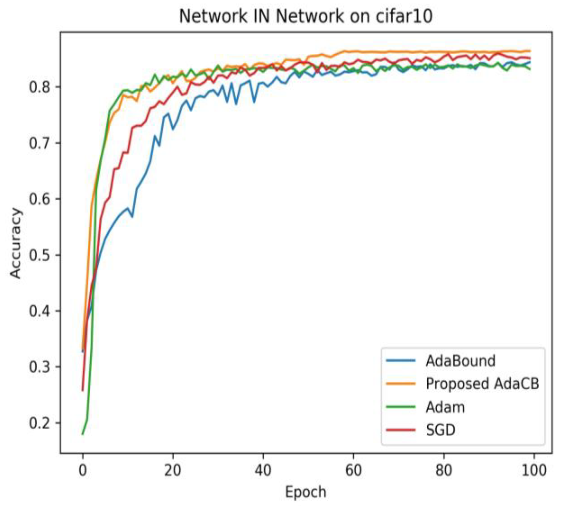
As we can see in
Figure 4, AdaBound has the worst convergence speed in the early stage and produces the worst testing accuracy on CIFAR10 under Network IN Network architecture. SGD (M) has a better convergence speed than AdaBound, and it finally beat AdaBound and Adam. AdaCB is as faster as Adam in the early stage and achieves the highest testing accuracy in the end. From
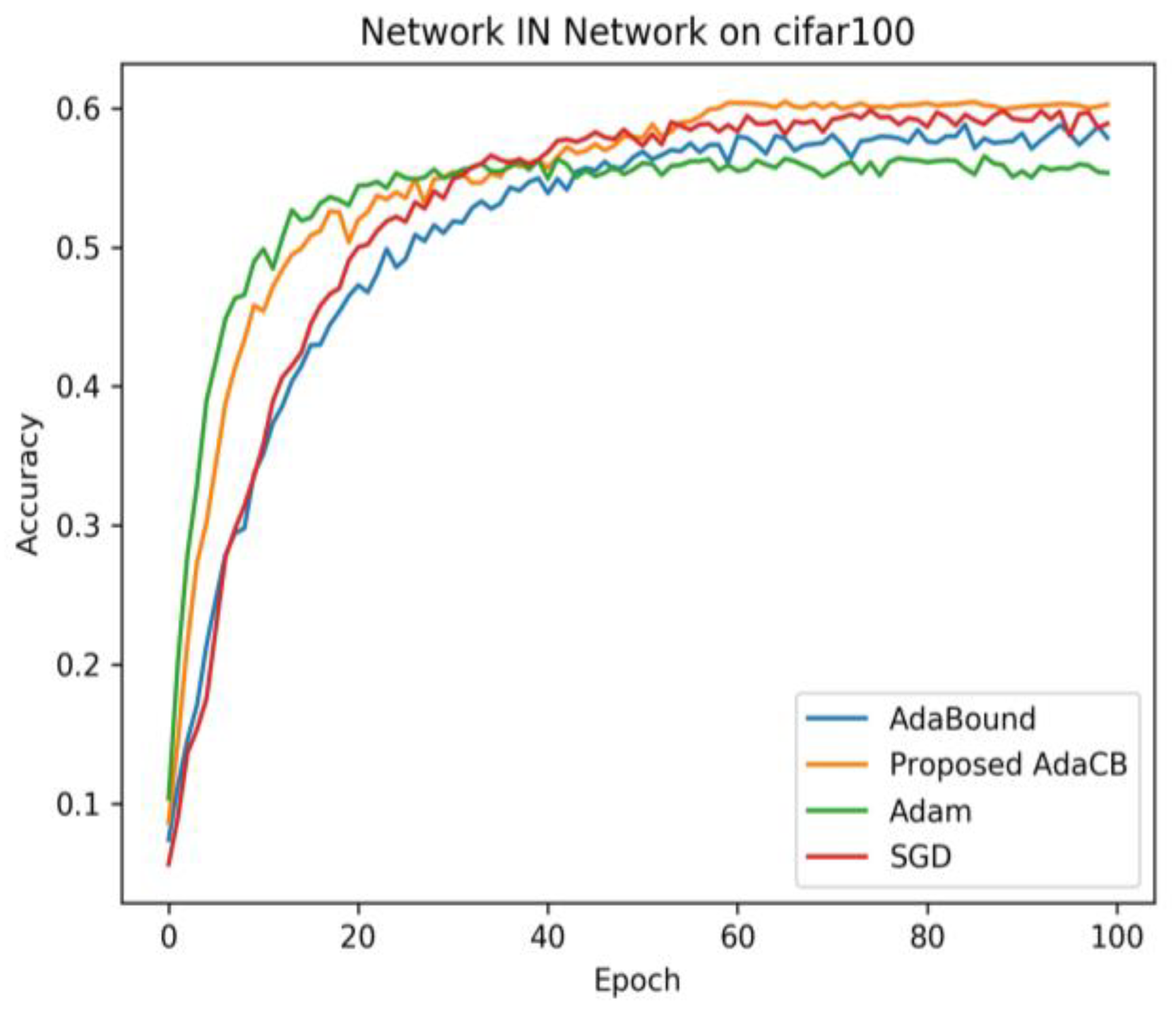
Figure 5, we can find that Adam has the fastest convergence speed in the early stage and the worst testing accuracy in the end. AdaCB is second only to Adam in convergence speed in the early stage, and it finally achieves the best testing accuracy on CIFAR100 under Network IN Network architecture. Adabound has a comparable convergence speed with SGD (M) before 20 epochs, and SGD (M) wins Adabound eventually.
Table 4 demonstrates the performance of each optimizer on CIFAR10 and CIFAR100 under Network IN Network.
4.5. Results of Resnet18 on CIFAR10 and CIFAR100
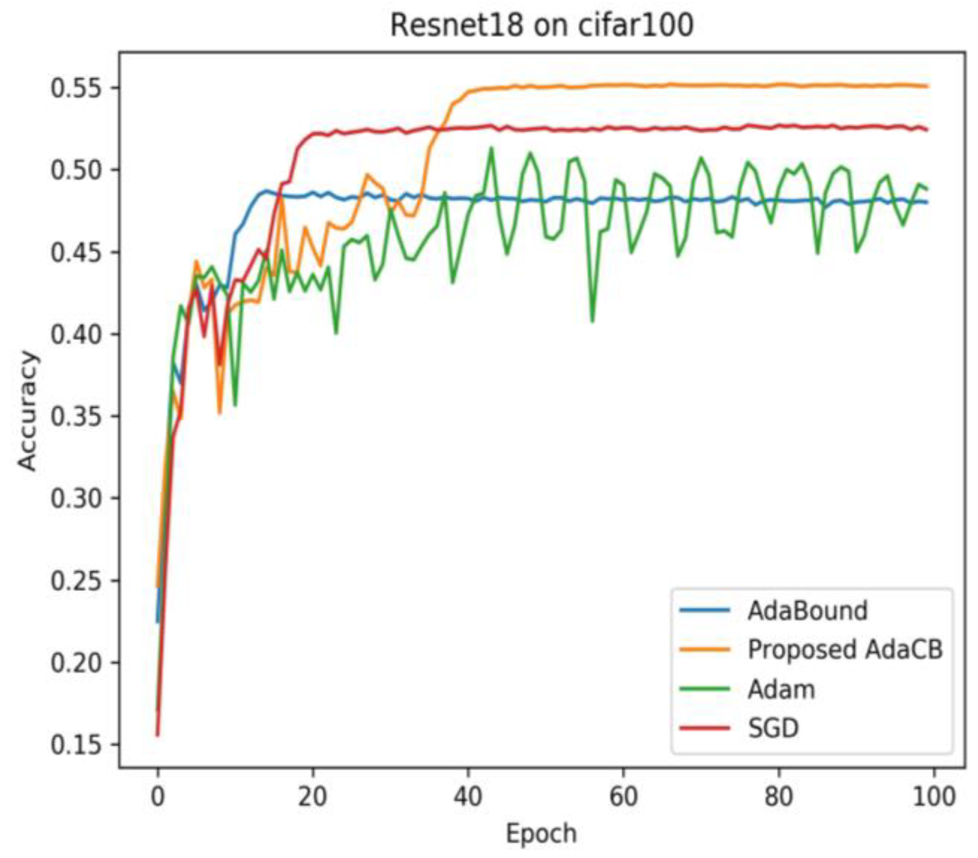
As we can see in
Figure 6 and
Figure 7, the testing accuracy of Adam is fluctuating on CIFAR10 and CIFAR100 under Resnet18 architecture. Adabound produces a smooth curve of testing accuracy, but its testing accuracy is the worst. AdaCB achieves the best testing accuracy, followed by SGD (M), Adam, and AdaBound. The results are shown in
Table 5.
5. Discussion
The experimental outcomes obtained from the last section have shown that AdaCB outperformed the other optimizers. Compared to Adam, our proposed method employs the two bounds to clip the learning rates of Adam, so the effect of unreasonable learning rates is alleviated during training. Additionally, compared to AdaBound, the bound functions of our method are designed based on reasonable convergence range obtained by the LR test instead of empirically hand designed, which can accurately truncate the unreasonable learning rates for a certain task. Moreover, our proposed method is faster than SGD (M) with convergence speed, because our method generates the feature of adaptive learning rates in the early stage. AdaCB integrates both advantages of the adaptive gradient descent method and SGD (M), which can behave like Adam in the early stage with faster convergence speed and become SGD (M) in the end with considerable accuracy. However, our method also has shortcomings. Our method relies on the LR test to pre-specify the convergence bound range, which takes a bit of time to train the current task with a few epochs to calculate the starting point and end point of the convergence range. In future work, we will investigate to determine the convergence bound range adaptively rather than pre-specify with the LR test, so more time can be saved.
6. Conclusions
In this paper, we proposed a new optimizer called AdaCB, which employs the convergence range bound on their effective learning rates. We compare our proposed method with Adam, AdaBound, and SGD (M) on CIFAR 10 and CIFAR 100 datasets across Smallnet, Network IN Network, and Resent. The outcomes indicate that our method outperforms other optimizers on CIFAR10 and CIFAR100 datasets with accuracies of (82.76%, 53.29%), (86.24%, 60.19%), and (83.24%, 55.04%) on Smallnet, Network IN Network and Resnet, respectively. Moreover, the proposed optimizer enjoys the convergence speed of Adam and generates considerable results like SGD (M).


