Article

Experimental Study on the Heat Transfer Performance of Various Magnet Arrangements in a Closed Space Filled with Ferrofluid

1
Graduate School of Mechanical Engineering, Sungkyunkwan University, Suwon 16419, Korea
2
Flow & Thermal Simulation Cell Team, Hyundai Mobis, Yongin 16891, Korea
3
School of Mechanical Engineering, Sungkyunkwan University, Suwon 16419, Korea
*
Authors to whom correspondence should be addressed.
Appl. Sci. 2022, 12(17), 8666; https://doi.org/10.3390/app12178666
Submission received: 4 August 2022 / Revised: 22 August 2022 / Accepted: 25 August 2022 / Published: 29 August 2022
(This article belongs to the Special Issue NANO KOREA 2022 in Applied Sciences)

Abstract

:
In this study, experiments, simulations, and optimization were performed to evaluate heat transfer performance of ferrofluids. Ferrofluids are colloidal suspensions containing magnetic-nano particles with a diameter of 5 to 15 nm in a base fluid such as oil or water. Recently, as many devices are miniaturized, the design of heat dissipation systems are being diversified to consider cost and safety, and it is becoming important to separate an ancillary device for cooling from main unit. In ferrofluids, the behavior and vortex of magnetic-nano particles are actively generated by an external magnetic field, and the cooling system can be designed in a simplified manner by using this characteristic. The main design parameter is the arrangement of permanent magnets, and the output variable is the temperature inside the magnetic nanofluid. The permanent magnet can be moved up and down, and the temperature inside the magnetic nanofluid was measured at various locations. A predictive model was created using a design of experiments (DOE) and response surface method (RSM) using selected design and temperature variables. Based on the generated regression model, an optimization was applied to find a permanent magnet arrangement that maximizes heat transfer performance. Through the optimization technique used in this study, economic efficiency in terms of time and cost was obtained by reducing the number of experiments.

1. Introduction

Recently, interest in safety issues of electronic devices has increased. This is because, as devices become smaller, risk of an explosion may occur if an efficient heat dissipation performance system cannot be built. To solve this problem, various studies of methods such as water cooling and air cooling have been conducted [1,2]. However, there is a limit to the method of uniformly distributing heat or cooling the device in the conventional way. In this study, an improved heat dissipation system was set by using a working fluid called a ferrofluid that can control the heat flow. A ferrofluid is a fluid, whose base fluid is water or oil, that is ferromagnetic because it contains ferromagnetic particles such as Fe 3 O 4 , Fe 2 O 3 , Gd 2 O 3 with a size of 3 to 15 nm [3]. Due to the magnetic particles, this fluid flows in a direction along with kinetic energy when an external magnetic field exists [4,5]. The thermal conductivity of a ferrofluid is also increased. Various studies using ferrofluids are being conducted due to the advantage of being able to control the flow in a desired direction to improve the heat transfer rate.
Singh et al. [6] used a ferrofluid and external magnetic fields to increase heat transfer on high temperature surfaces of solar photovoltaic (PV) systems. Parameter sets were set as actuation frequency of alternating magnetic field (0.5~20 Hz), Reynolds number (Re = 24, 60 and 100). Using velocity and temperature contours, results were visually compared depending on whether magnetic field was applied. When an electromagnet was applied, numerical results were compared and analyzed by increasing Re or changing the frequency. Through this, a difference in the heat transfer performance between the high temperature ferrofluid and the low temperature wall was confirmed. Finally, compared with the case where no electromagnet was applied, the heat transfer was increased by 17.41% in the case of Re = 100 and magnetic flux density (B) = 1 T.
Heidari et al. [7] set up a new cooling system for PV systems using a ferrofluid composed of Fe 3 O 4 based on pure deionized water (DIW) as a cooling medium and a rotating magnetic field (RMF). The experimental setup consisted of four major components. There was a PV system that generated heat, a metal halide lamp, a ferrofluid and permanent magnets. The design variables were the concentration of magnetic nano particles (MNPs = 0.01, 0.02, 0.03, 0.04, 0.05%), the rotational speed of magnet, and the magnetic field induction (B = 0.35, 0.45, 0.57, 0.72, 0.88 T). The system consisted of 72 cells, and 12 temperature measurement points were set. Overall, the cooling performance of the cell surface was improved as the concentration of magnetic nano particles, the strength of the magnetic flux density, and the rotation speed increased. This was due to the performance change by the magnetic torque of particles and the vorticity of the ferrofluid. Finally, a cooling performance improvement of 17.8~30% and a maximum power improvement of 1.67~47.5% was shown.
Bezaatpour et al. [8] tried to improve the performance of a flat plate solar collector by using four rotary tubes and a magnetic field inducer. As the working fluid inside the collector tube, a ferrofluid composed of Fe 3 O 4 and water was used. The design parameters were set as the tube rotation speed ( ω = 0~2.5 rpm) and magnetic field intensity (B = 0~8 mT). Heat dissipation occurred through an external magnetic field and tube rotation, and the performance was improved by setting the convective heat transfer coefficient as an output parameter. In conclusion, 27.8% and 10.44% of energy loss was recovered by using a magnetic field inducer and a rotary pipe, respectively.
Mehrez et al. [9] analyzed the heat transfer performance using a low temperature ferrofluid flowing in a rectangular horizontal channel. Design parameters include nanoparticles volume fractions ( φ = 0~0.05), Reynolds number (Re = 50~500), and magnetic number (Mn = 0~100). Heat exchange became active by using a magnetic field and the ferrofluid. This is because a recirculation region was created around the magnetic source and the thermal boundary layer was removed. Finally, compared to the case without an external magnetic field, the heat exchange increased by 20% at φ = 0.05. In addition, in the case of φ = 0.05 and Re = 500, the heat transfer performance was improved by 86%.
Ashjaee et al. [10] experimentally studied laminar forced convection using a ferrofluid by applying an external magnetic field around a small heat sink device. The magnetic field area was visually confirmed using the commercial program COMSOL Multiphysics. In addition, the temperature of the heat sink was measured by using thermocouple wire and a data logger. The magnetic field strength and Re were set as variables to analyze the heat transfer performance by the ferrofluid. In the presence of an external fixed magnetic field, the magnetic nanoparticles were maintained in a constant arrangement towards the magnetic field in the base fluid. Finally, the thermal conductivity of the ferrofluid was increased by the magnetic field, thereby improving the heat transfer performance.
Ghorbani et al. [11] set the magnetic field strength and position as variables and studied the heat transfer performance of high temperature ferrofluid when it flowed over a cold wall. The magnetic field strength was set to five variables and the location to six variables. The higher the magnetic field strength, the better the heat transfer performance. The heat exchange was most active when all magnets were located on the cold wall. This is because small circulation is combined around the magnet to create a big vortex, and the temperature exchange is activated by this vortex. Finally, the cooling rate was increased.
Studies have been recently conducted comparing the heat transfer performance of ferrofluids under different arrangements of magnets. However, studies comparing the performance of ferrofluids based on optimization techniques are insufficient [12]. Therefore, the experimental results were analyzed according to the arrangement of external permanent magnets after containing the ferrofluid in a glass tube. Based on this, an arrangement of permanent magnets with optimal heat dissipation performance was found by utilizing optimization techniques such as design of experiments (DOE) and response surface method (RSM).

2. Experimental Process

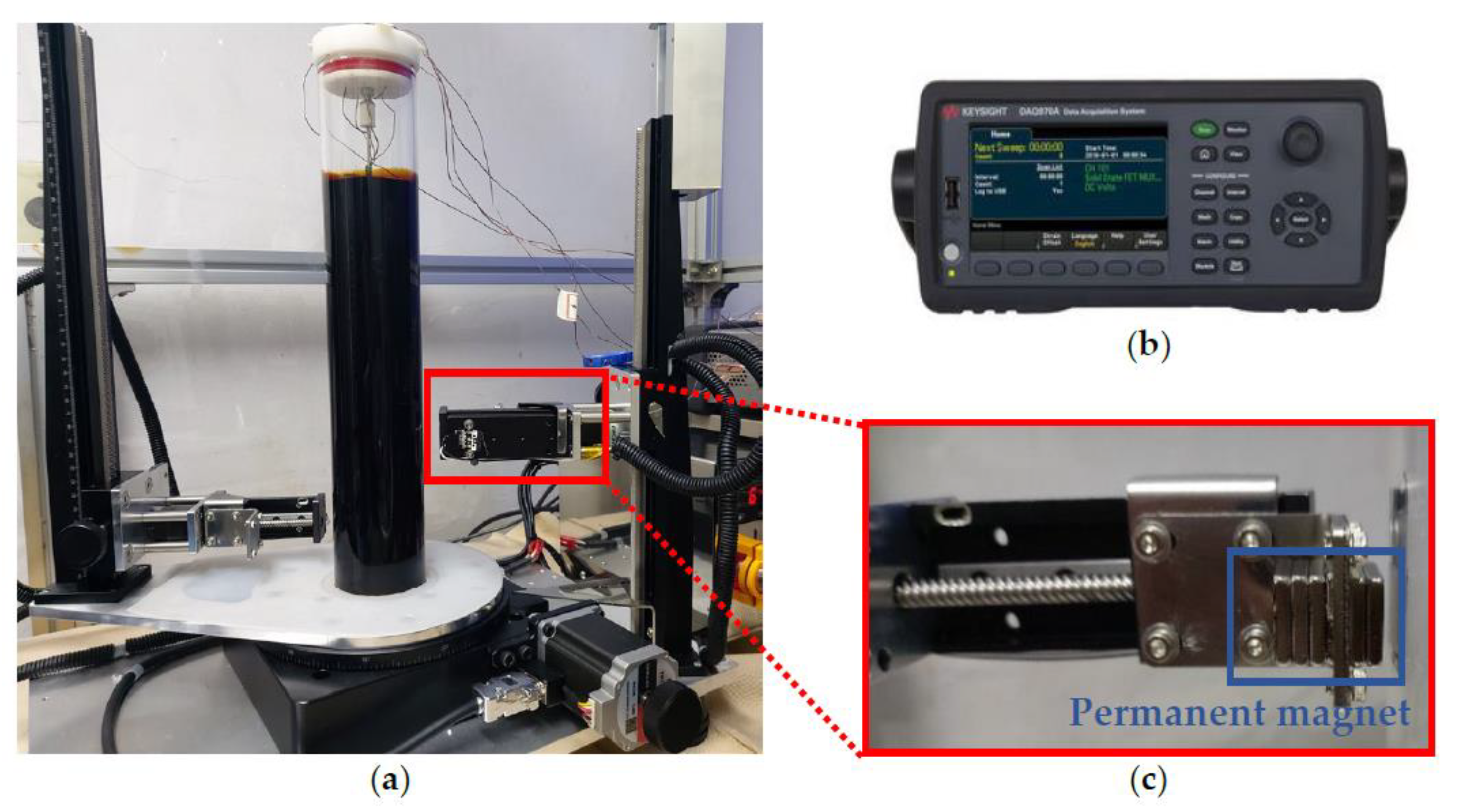
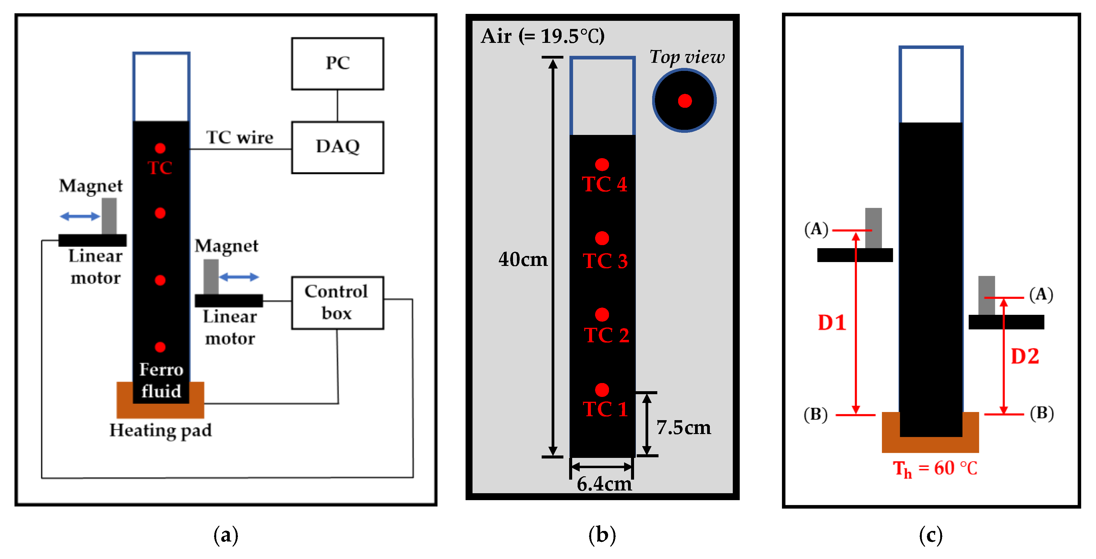
2.1. Experimental Device

In this study, a ferrofluid was used as the heat transfer medium. It was a colloidal solution containing Fe 3 O 4 magnetic nanoparticles with a size of 5 to 15 nm in an oil-based base fluid called EFH-1. It was composed of iron oxide magnetite, oleic acid dispersant, hydrotreated light distillate. Surfactant treatment was applied to prevent agglomeration between particles. Table 1 shows the physical properties of EFH-1 [13]. It has a property of increasing thermal conductivity when an external magnetic field is applied, so heat transfer performance can be improved by using ferrofluid. The overall experimental setup is shown in Figure 1a. To contain the ferrofluid, a Pyrex glass tube with high heat resistance was used. The temperature deviation was set to compare the heat transfer performance inside the glass tube according to the arrangement of permanent magnets. A heating pad was placed to transfer high temperature heat to the lower portion of the glass tube. The heating pad was the principle of generating heat by the internal coil. This device can set the target temperature through the control box. Permanent magnets were placed around the glass tube to apply an external magnetic field. Neodymium permanent magnets (20 mm × 15 mm × 3 mm) were used, and they were arranged as shown in Figure 1c. The magnetic field strength was set to 0.325 T. When permanent magnets are fixed in one position without movement, magnetic nanoparticles aggregate only around the magnets, and the fluidity of the ferrofluid is limited. Therefore, linear motors were used to ensure the dispersion of the particles and to promote heat exchange by the fluid. Permanent magnets were placed on the front side of the motors; the magnets moved according to the reciprocating motion of motors. Through various arrangements of the permanent magnets, the behavior of the ferrofluid inside the glass tube could be diversified, thereby affecting the heat transfer performance. A T-type thermocouple TC wire was used to measure the temperature inside the glass tube in real time. The TC wires were placed at four points at regular height intervals, and the location was set at the center of the glass tube. The temperature data obtained from the TC wires was confirmed in real time through a data acquisition system DAQ (DAQ970A, of Keysight). Temperature data using the DAQ was measured and stored at 2 s cycle.

2.2. Experimental Procedure

For the experiment, the glass tube was filled with the ferrofluid to 80% of its height (40 cm). Four TC wires for real time temperature measurement were arranged at equal intervals of 7.5 cm from the bottom of the glass tube as shown in Figure 2b. In this experiment, the temperature deviation at the glass tube was set using the outside air and heating pad. The outside temperature (air) was maintained at 19.5 °C (±0.1 °C) during the experiment. The heating pad was placed at the bottom of the tube as shown in Figure 2a, and the experiment was conducted by setting T h (=60 °C) as the reference temperature. The linear motor installed for the permanent magnet movement was set to reciprocate at a speed of 17.5 cm/s to maximize the movement of ferrofluid (Table 2). The experiment was conducted for 4 h and 30 min for each case to obtain converged result for all cases.

2.3. Design of Experiments

To analyze the heat transfer performance according to the permanent magnet arrangement, a design of experiments (DOE) was conducted [14]. As design parameters, the height of permanent magnets (D1, D2 of Figure 2c) was set. The center position of the permanent magnet was set to (A), and the upper surface of the heating pad was set to (B) (see Figure 2c). Based on the glass tube, the distance corresponding to the side is D1, and to the right side is D2. The DOE was processed using Ansys Design Xplorer software. Latin hypercube sampling (LHS) was selected as the DOE type, and the parameter sets for the design variables (height of the permanent magnet) were set according to LHS. The advantage of LHS is the permanent magnet arrangement can be randomly determined without overlapping the design points between the parameter sets. Nine experiments were conducted with different permanent magnet arrangements (see Table 3). The resulting temperature for each of the TC wires in each experiment is shown in Table 4. In experiment 4 and 8, it was numerically confirmed that temperature was high. Based on this result, an optimization process was performed.
In addition, we considered two experimental uncertainties; the random error was the permanent magnet vertical position adjustment (D1, D2), and the systematic error was the measurement error caused by the thermocouple (TC). It was assumed that a random error occurs about 0.25 mm in the D1 and D2 adjustment. The uncertainty of the TC is known to be about 0.013 °C at 0.006 mV/°C at 25 °C and was ignored.

3. Numerical Analysis

3.1. Governing Equations

Prior to the experiment, numerical analysis was performed using the COMSOL Multiphysics, CFD (Computational Fluid Dynamics) commercial software program. Numerical analysis was set under the same conditions as the experiment. To analyze changes according to the vertical arrangement of permanent magnets, numerical analysis was performed in 2D. The equations for continuity, momentum, and energy are as follows [15]:
-
Continuity:
· ( ρ V ) = 0  
-
Momentum:
· ( ρ V V ) = · μ ( ( V ) T + V ) p 2 3 μ ( · V ) I + F
-
Energy:
· ( V ( p + ρ E ) ) = · ( ( τ = · V ) + k T h j J j ) + S h
The last F term of momentum Equation (2) is the force term that corresponds to both the buoyancy force and the magnetic force. Therefore, the F term can be replaced with the sum of ρ β ( T T r e f ) corresponding to buoyancy force and ( M · ) B corresponding to magnetic force. The final Equation (2) with these terms is as follows:
-
Momentum:
· ( ρ V V ) = · μ ( ( V ) T + V ) p 2 3 μ ( · V ) I + ρ β ( T T r e f )   + ( M · ) B
Additionally, the expression for Gauss’s laws is as follows [16]:
B = μ 0 ( M + H )  
where B is the magnetic flux density, M is the magnetization, and H is the magnetic field strength. Furthermore, μ 0 is a constant value, meaning a permeability value in a vacuum state (= 4 π × 10 7 ); B and H as expressions for Maxwell’s equation, respectively, are as follows [17]:
· B = 0
  × H = 0
Moreover, the relation for M and H in Equation (5) is expressed as follows:
M = χ m H  
In Equation (8), χ m is the magnetic susceptibility, and is defined as follows [18]:
χ m = χ 0 1 + β ( T T 0 )  
In this expression, β means a thermal expansion coefficient, and it is confirmed that an inverse relationship between χ m and T is established. This is, high temperature ferrofluid responds loss to the external magnetic field, and low temperature fluid actively responds to the magnetic field. Due to these characteristics, the convection phenomenon occurring in the magnetic field is called a thermomagnetic convection, and it promotes heat exchange.

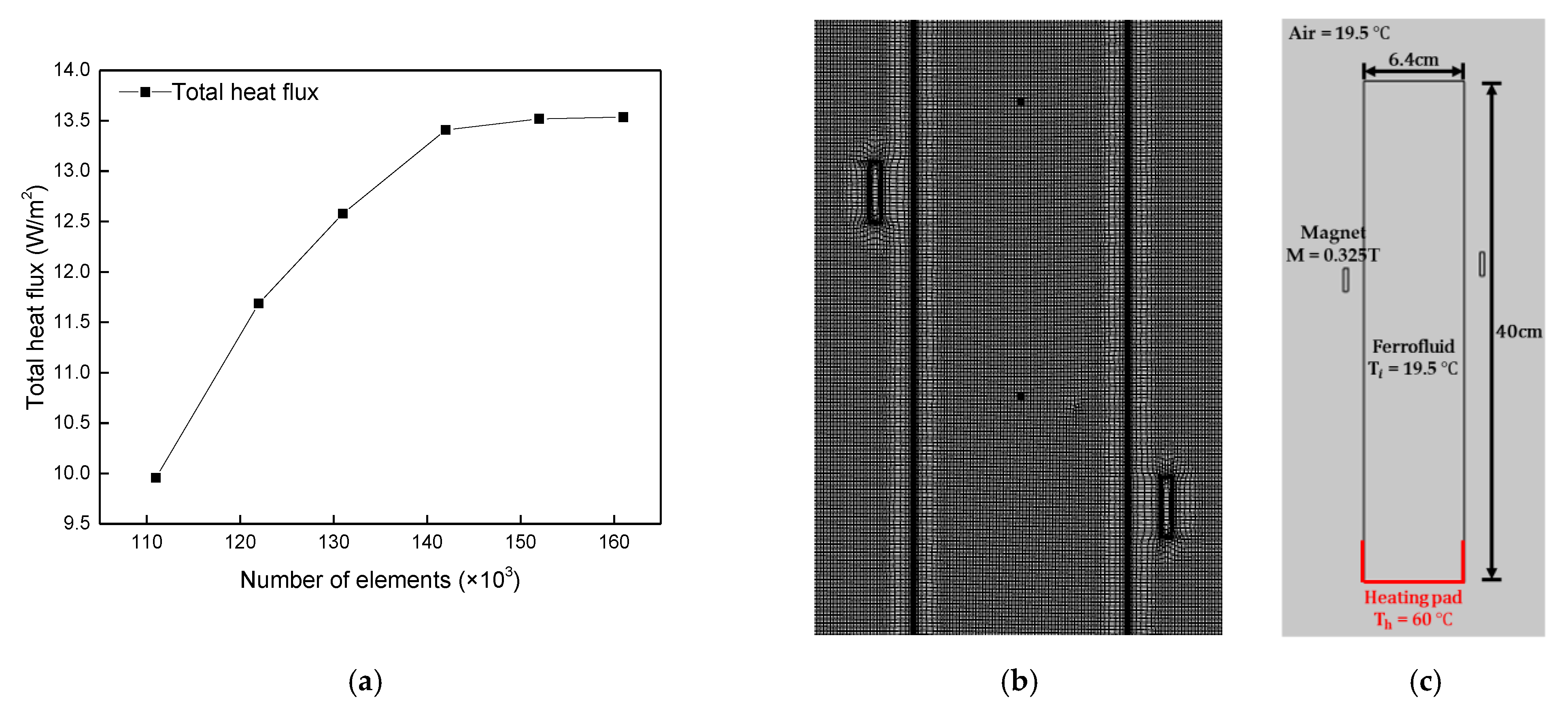
3.2. Grid Systems and Operating Conditions

To reduce the simulation result error, a grid dependency test was conducted. This process was carried out six times. As shown in Figure 3a, the x-axis of the graph is the number of elements, and the y-axis is the total heat flux. Starting with about 110,000 elements, the number of elements was increased by about 100,000 and the results were analyzed. As a result, there was an error in the previous three cases. After about 140,000 elements, it was determined that the total heat flux converged to about 13.5 W/m2. Therefore, numerical analysis was performed on about 140,000 elements in consideration of time and efficiency. Additionally, eight inflation layers were arranged to precisely observe the flow pattern around the permanent magnets and the wall of the glass tube. Finally, mesh configurations in these conditions are shown in Figure 3b. The operating conditions and boundary conditions of the simulation were basically set to the same as those of the experiment. As shown Figure 3c, the heating pad temperature T h (=60 °C) at the lower part of the glass tube and the initial temperature T i   (=19.5 °C) of the ferrofluid were set as in the experiment, and the magnetic flux density (M) of the permanent magnet was set to 0.325 T. Since the effect of the outside temperature was not large in the actual experiment, the boundary condition of the glass tube except for the heating pad were assumed to be walls in the simulation. Then, numerical analysis was performed.

4. Optimization Process

4.1. Response Surface Methods

In this study, a response surface based on design of experiments was created. A neural network (NN) and a non-parametric regression (NPR) method were used to generate the response surface [19,20,21].
The first regression method is a neural network. The NN’s fundamental schematic is shown in Figure 4. Three layers make up a NN: the input side, the hidden layer, and the output layer. A hidden layer may include one or more layers, and a NN is trained by establishing mathematical connections and weights between neighboring layers. The hidden layer’s layers repeat learning and provide the output layer with the chosen input. When building a regression model, 70% of the data are used for training and 30% are used for checking. For nonlinear issues, NN-based regression has a high success rate. The number of layers was one of the NN factors that were changed for this investigation.
The second method is a non-parametric regression. In contrast to previous RSM approaches, the non-parametric regression method estimates the values of the one design point that must be determined. Error in a particular data set can be reduced or eliminated using this kind of non-parametric regression analysis. This enables the creation of a regression model that is more like the original data. The basic formula of NPR method is as follows:
f ( X ) = W , X + b = i = 1 N ( A i A i * ) * K ( X i , X ) + b
Here W is weighting factor, X is input sample from DOE, b is bias, K is Gaussian kernel, A is Lagrange multipliers, N is number of DOE points, a and b are the unknown parameters.

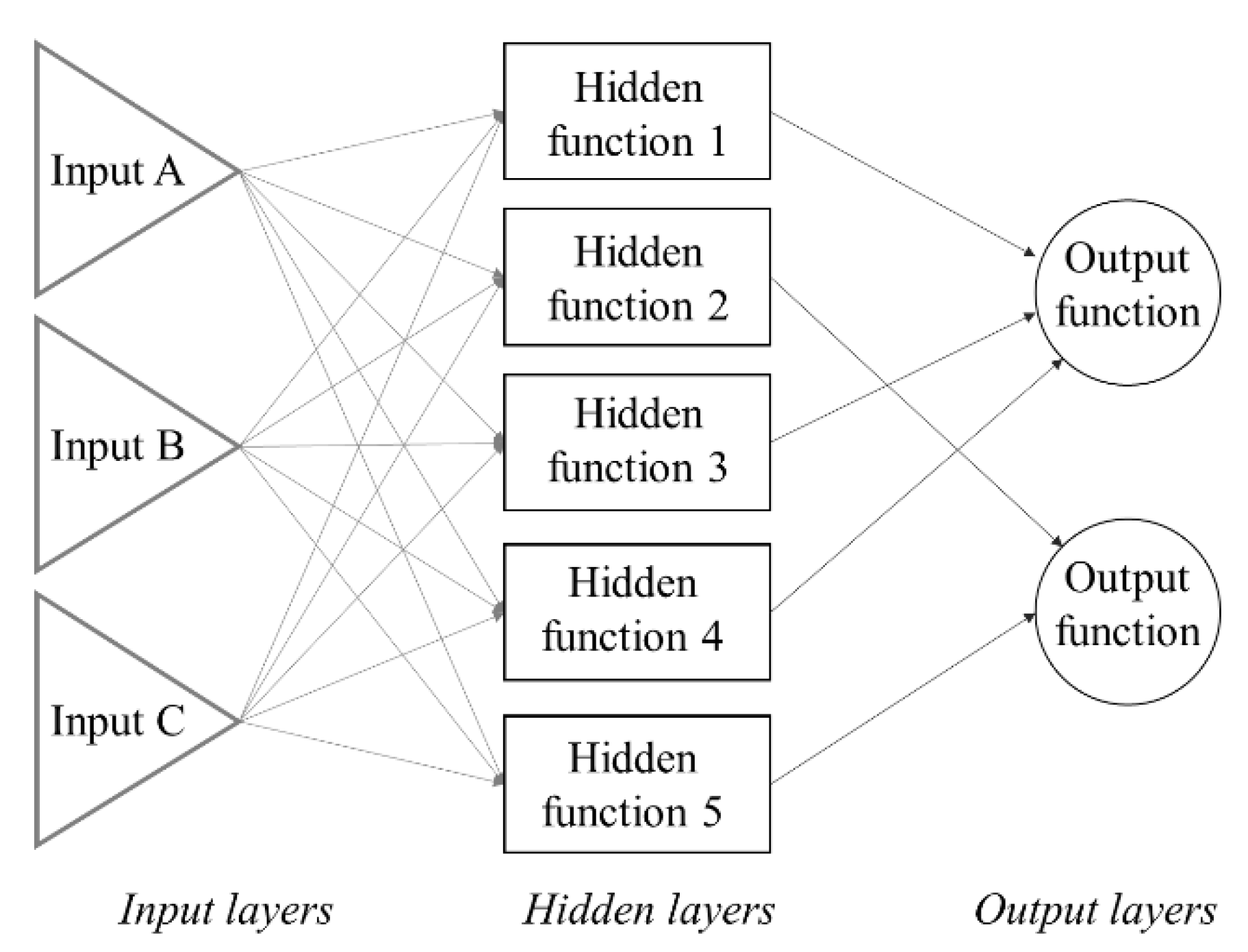
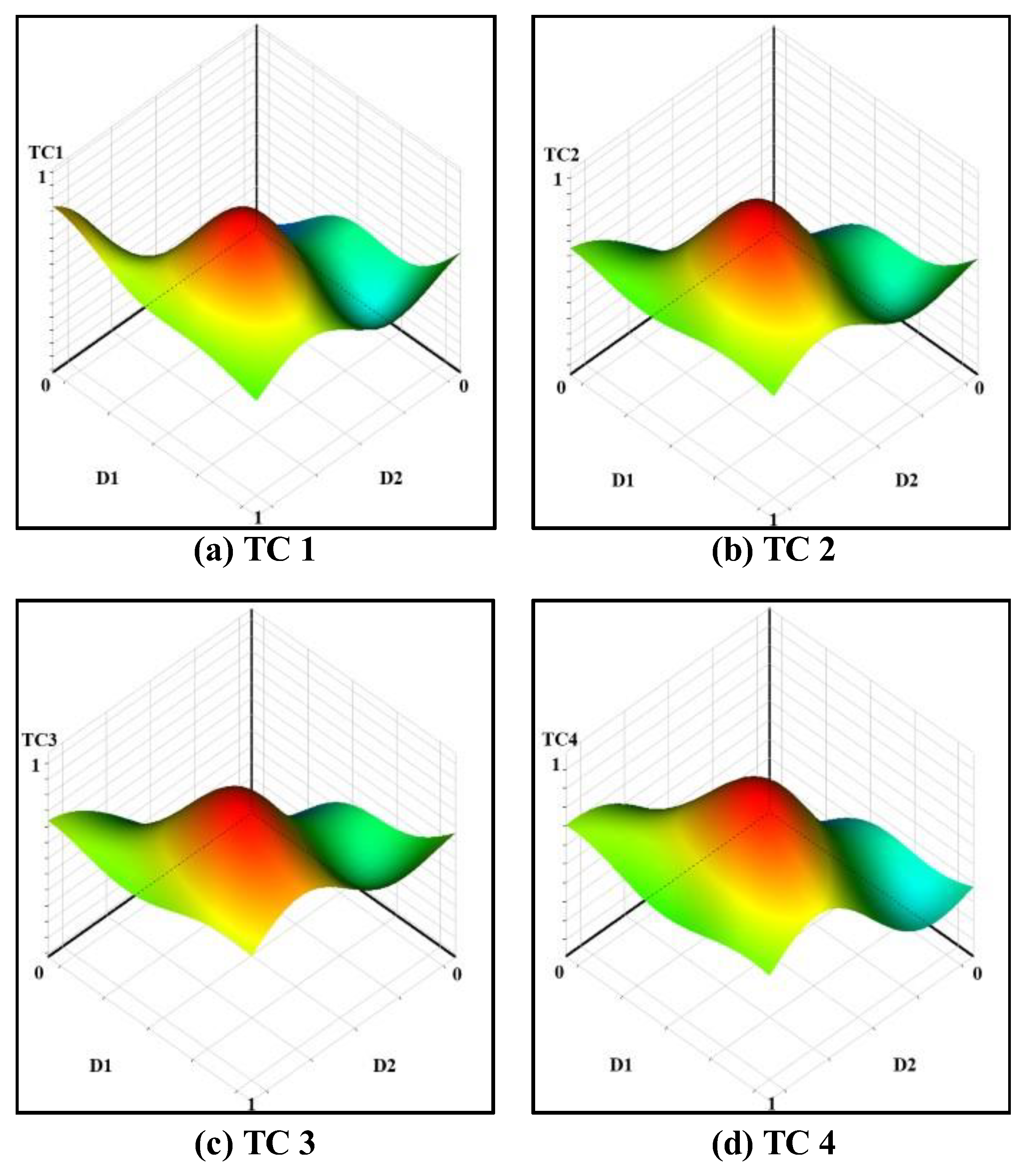
4.2. Response Surface Result of Neural Networks

Figure 5 shows the response surface using the NN method. The x-axis means D1, the y-axis means D2, and the z-axis means values from TC1 to TC4, respectively. For (a) TC1 and (b) TC2, the overall trend was very similar. As the D1 value increased, the temperature of TC1 increased, and the maximum point of the temperature value was shown at D1 and D2 = 25. (c) TC3 and (d) TC4 showed a similar relationship. The maximum point was shown when D1 was a low value, and the maximum point was shown when D2.

4.3. Response Surface Result of Non-Parametric Regression

Figure 6 shows the response surface using the NPR method. In the case of the NPR method, an overall similar trend was shown from TC1 to TC4. In the case of D1, the maximum TC value was shown at about 16, and in the case of D2, the maximum TC value was shown at about 20.

4.4. Accuracy of Response Surface

Root mean square error (RMSE) and coefficient of determination (R2) were used to evaluate the regression models. Both methods are generally used to assess the correctness of a regression model, and the formula is as follows [22]:
RMSE = 1 N i = 1 N ( y i y i ^ ) 2
R 2 = i = 1 N ( y i y i ^ ) 2 i = 1 N ( y i y i ¯ ) 2
where y i is the function value of an experimental point’s response variable, y i ^ is the function value of the regression model and N represents the number of design points for the regression model evaluation.
Figure 7 schematically shows the goodness of fit for the three regression models. Each figure (circle, diamond) for the two regression models is a generalized distribution for four output variables (see Table 5). The x-axis and y-axis denote normalized test and predicted data, and it can be judged that the prediction is better the more it matches the x = y line. It can be judged that the NPR method better predicts the data. Based on this result, the regression model to be used for optimization was selected as NPR.

4.5. Optimization Formula

In this optimization, the screening method was used. The screening is non-iterative sampling method using a quasi-random number generator. Besides, it can be available for both continuous and discrete input parameters. The objective function in the optimization of this study is to maximize the temperature of TC4 that is farthest from the floor. This is to ensure that the optimized magnet arrangement produces the best heat transfer. As a constraint, the temperature of the remaining TC1~TC3 should be raised to 35 degrees or higher. The optimization formula is as follows:
Find   D i   ( i = 1 , 2 ) To maximize T C 4 Subject to T C 1 > 35   ( ° ) T C 2 > 35   ( ° ) T C 3 > 35   ( ° ) 3.6   <   D 1   <   26.66   ( c m ) 3.6   <   D 2   <   26.66   ( c m )

5. Results and Discussion

5.1. Optimization Results

Table 6 shows the test results based on the optimal values (D1, D2) predicted by the two regression models. Both NN and NPR predicted temperatures above 35 °C from TC1 to TC4, but in the actual experimental results, there was no result exceeding 35 °C in the case of the NN model. However, in the NPR result, it can be judged that the temperature of 35 °C or higher was measured in the actual test from TC1 to TC3, and it is consistent with the constraints condition of this optimization.
The relative errors of the two regression models were compared. The average relative error (predict vs. exp.) occurred about 1.5% in the NN models TC1 to TC4, but the relative error in the NPR model was 0.6%. In Figure 7, the goodness-of-fit results showed that the NPR model had a higher fit, which was also confirmed by the experimental results.
In the case of TC4 temperature, which is the objective of this optimization, the NPR model showed better results in this optimization because a higher temperature was measured in the NPR model (34.99 °C) compared to the NN model (34.57 °C).

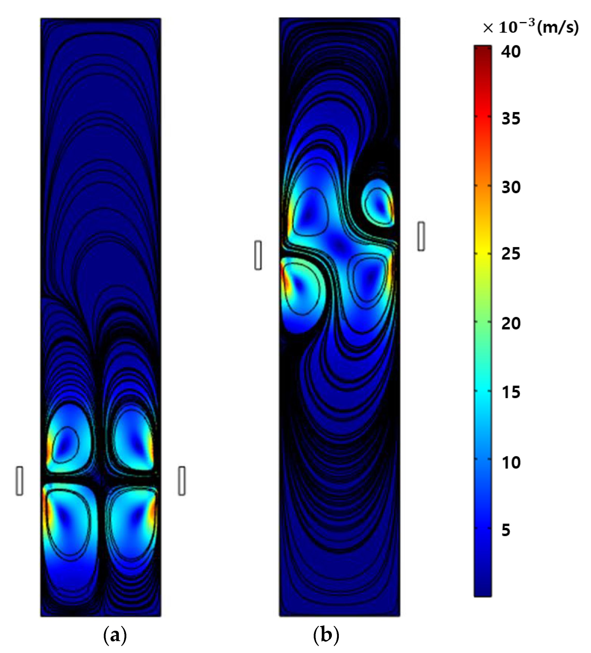
5.2. Numerical Results

To verify the reliability of the numerical analysis, experimental values and simulation values were compared for NPR (the permanent magnets arrangement of the highest temperature distribution) and experiment 3 (the arrangement of the lowest temperature distribution) in Table 7. Only an error of maximum 1.08% was shown, proving the validity of the numerical analysis results.
The velocity contour was used to visualize the behavior of the ferrofluid in the Pyrex glass tube. Numerical analysis was performed for all experiments. Figure 8 shows two experiments (experiment 3 and NPR) among them. In experiment 3 (see Figure 8a), most of the fluid behavior is located at the bottom of the glass tube. There were cells only near permanent magnets, and heat diffusion of the fluid was concentrated near there. The high-temperature fluid in the lower part could not reach the upper part of the tube. Therefore, the overall temperature distribution was low. In the case of NPR (see Figure 8b), the fluid behavior was different from experiment 3. The fluid concentration around the permanent magnets was similar to experiment 3, but there was a difference in that ferrofluid circulated over a wide range in the tube. An eddy was actively generated by the external magnetic field. It means that the high-temperature fluid at the bottom affected the upper part of the tube. That is, the energy exchange occurred most actively, and the temperature distribution was the highest. Through numerical analysis, the variation of the fluid behavior was confirmed according to the arrangement of permanent magnets.

6. Conclusions

In this study, experiments, numerical analysis, and optimization were performed using a ferrofluid that has the advantage of controlling flow by a magnetic field.
The vertical arrangement of permanent magnets around the glass tube containing the magnetic fluid was selected as the design variable (input variable), and TC1 to TC4 for measuring the temperature of the magnetic fluid were selected as the temperature variable (output variable).
Design of experiments (DOE) was performed to establish experimental points for the permanent arrangement. Among various DOE methods, Latin hypercube sampling (LHS), which has the advantage of predicting the population well even with a small sample, was selected. Experiments were conducted with a total of nine experimental arrangements derived through this method (refer to Table 3). As a result, in experiment 4, the temperature distribution was the highest in the four TCs (see Table 4). In particular, it was measured about 34.95 °C at TC 4. That means the heat diffusion was actively distributed to the top of the glass tube. On the other hand, experiment 3 had the lowest temperature at TC 4, about 34.01 °C. Through this, it was determined that the circulation of the ferrofluid did not occur well when permanent magnets were placed at the bottom of the glass tube (D1, D2 = 5.3 cm).
To determine the arrangement of permanent magnets in which optimal heat diffusion occurs, an optimal design based on the response surface method was performed.
For the regression of the response surface method, two methods (NN, NPR) were performed. The maximum temperature of TC4 was obtained by setting the range of temperature from TC1~TC3 and constraints of the design variables D1 and D2. Through the process, temperature values for NN and NPR were derived.
As a result of optimization, when the arrangement of D1 and D2 was 17.78 cm and 18.8 cm, thermal diffusion results of more than 35 °C were predicted for both TC1 and TC4. In the experiment results, the average relative error of TC1~TC4 was about 0.6% compared to the predicted value, from which it can be judged that the optimal value prediction of the NPR model was good.
Numerical analysis was performed by reflecting the optimization results. The lowest (experiment 3) and highest (NPR) temperature distribution were intensively compared. In the case of NPR, the fluid behavior formed cell shapes throughout the glass tube in a relatively wide range. Through this, the heat diffusion occurred actively, and the temperature distribution was high.

Author Contributions

Conceptualization, H.-S.K. and Y.-S.C.; methodology, H.-S.K. and Y.-S.C.; software, H.-S.K. and Y.-S.C.; validation, H.-S.K.; formal analysis, Y.-S.C.; investigation, Y.-S.C.; resources, H.-S.K.; data curation, H.-S.S.; writing—original draft preparation, Y.-S.C.; writing—review and editing, H.-S.K. and Y.-S.C.; visualization, H.-S.K.; supervision, Y.-J.K.; project administration, Y.-J.K.; funding acquisition, Y.-J.K. All authors have read and agreed to the published version of the manuscript.

Funding

This research was funded by the National Research Foundation of Korea (NRF), grant number (No. NRF-2021R1A2C1010499).

Institutional Review Board Statement

Not applicable.

Informed Consent Statement

Not applicable.

Data Availability Statement

Not applicable.

Conflicts of Interest

The authors declare no conflict of interest.

References

  1. Tang, G.; Han, Y.; Lau, B.L.; Zhang, X.; Rhee, D.M. An efficient single phase liquid cooling system for microelectronic devices with high power chip. In Proceedings of the 17th Electronics Packaging and Technology Conference (EPTC), Singapore, 2–4 December 2015; pp. 1–6. [Google Scholar]
  2. Marcinichen, J.B.; Olivier, J.A.; Thome, J.R. On-chip two-phase cooling of datacenters: Cooling system and energy recovery evaluation. Appl. Therm. Eng. 2012, 41, 36–51. [Google Scholar] [CrossRef]
  3. Pislaru-Danescu, L.; Morega, A.; Telipan, G.; Stoica, V. Nanoparticles of ferrofluid Fe3O4 synthetised by coprecipitation method used in microactuation process. Optoelectron Adv. Mater. 2010, 8, 1182–1186. [Google Scholar]
  4. Sheikhnejad, Y.; Hosseini, R.; Avval, M.S. Experimental study on heat transfer enhancement of laminar ferrofluid flow in horizontal tube partially filled porous media under fixed parallel magnet bars. J. Magn. Magn. Mater. 2017, 424, 16–25. [Google Scholar] [CrossRef]
  5. Choi, Y.S.; Kim, Y.J. Effect of Magnetic Nanofluids on the Performance of a Fin-Tube Heat Exchanger. Appl. Sci. 2021, 11, 9261. [Google Scholar] [CrossRef]
  6. Singh, D.; Shyam, S.; Mehta, B.; Asfer, M.; Alshqirate, A.S. Exploring heat transfer characteristics of ferrofluid in the presence of magnetic field for cooling of solar photovoltaic systems. J. Therm. Sci. Eng. Appl. 2019, 11, 041017. [Google Scholar] [CrossRef]
  7. Heidari, N.; Rahimi, M.; Azimi, N. Experimental investigation on using ferrofluid and rotating magnetic field (RMF) for cooling enhancement in a photovoltaic cell. Int. Commun. Heat Mass Transf. 2018, 94, 32–38. [Google Scholar] [CrossRef]
  8. Bezaatpour, M.; Rostamzadeh, H. Design and evaluation of flat plate solar collector equipped with nanofluid, rotary tube, and magnetic field inducer in a cold region. Renew. Energy 2021, 170, 574–586. [Google Scholar] [CrossRef]
  9. Mehrez, Z.; El Cafsi, A. Heat exchange enhancement of ferrofluid flow into rectangular channel in the presence of a magnetic field. Appl. Math. Comput. 2021, 391, 125634. [Google Scholar] [CrossRef]
  10. Ashjaee, M.; Goharkhah, M.; Khadem, L.A.; Ahmadi, R. Effect of magnetic field on the forced convection heat transfer and pressure drop of a magnetic nanofluid in a miniature heat sink. Heat Mass Transf. 2015, 51, 953–964. [Google Scholar] [CrossRef]
  11. Ghorbani, B.; Ebrahimi, S.; Vijayaraghavan, K. CFD modeling and sensitivity analysis of heat transfer enhancement of a ferrofluid flow in the presence of a magnetic field. Int. J. Heat Mass Transf. 2018, 127, 544–552. [Google Scholar] [CrossRef]
  12. Pathak, S.; Zhang, R.; Bun, K.; Zhang, H.; Gayen, B.; Wang, X. Development of a novel wind to electrical energy converter of passive ferrofluid levitation through its parameter modelling and optimization. Sustain. Energy Technol. Assess. 2021, 48, 101641. [Google Scholar] [CrossRef]
  13. Lee, M.; Kim, Y.J. Thermomagnetic convection of ferrofluid in an enclosure channel with an internal magnetic field. Micromachines 2019, 10, 553. [Google Scholar] [CrossRef] [PubMed]
  14. Lyu, Q.; Xiao, Z.; Zeng, Q.; Xiao, L.; Long, X. Implementation of design of experiment for structural optimization of annular jet pump. J. Mech. Sci. Technol. 2016, 30, 585–592. [Google Scholar] [CrossRef]
  15. Sheikholeslami, M.; Gerdroodbary, M.B.; Mousavi, S.V.; Ganji, D.D.; Moradi, R. Heat transfer enhancement of ferrofluid inside an 90 elbow channel by non-uniform magnetic field. J. Magn. Magn. Mater. 2018, 460, 302–311. [Google Scholar] [CrossRef]
  16. Cheng, Y.; Li, D. Experimental investigation on convection heat transfer characteristics of ferrofluid in a horizontal channel under a non-uniform magnetic field. Appl. Therm. Eng. 2019, 163, 114306. [Google Scholar] [CrossRef]
  17. Szabo, P.S.; Früh, W.G. The transition from natural convection to thermomagnetic convection of a magnetic fluid in a non-uniform magnetic field. J. Magn. Magn. Mater. 2018, 447, 116–123. [Google Scholar] [CrossRef]
  18. Bezaatpour, M.; Goharkhah, M. Convective heat transfer enhancement in a double pipe mini heat exchanger by magnetic field induced swirling flow. Appl. Therm. Eng. 2020, 167, 114801. [Google Scholar] [CrossRef]
  19. Liu, Y.; Shimoda, M.; Shibutani, Y. Parameter-free method for the shape optimization of stiffeners on thin-walled structures to minimize stress concentration. J. Mech. Sci. Technol. 2015, 29, 1383–1390. [Google Scholar] [CrossRef]
  20. Green, P.J.; Silverman, B.W. Generalized Linear Models and Nonparametric Regression; Chapman and Hall: New York, NY, USA, 1994. [Google Scholar]
  21. Kang, H.S.; Kim, Y.J. Optimal design of impeller for centrifugal compressor under the influence of one-way fluid-structure interaction. J. Mech. Sci. Technol. 2016, 30, 3953–3959. [Google Scholar] [CrossRef]
  22. Malekan, M.; Khosravi, A. Investigation of convective heat transfer of ferrofluid using CFD simulation and adaptive neuro-fuzzy inference system optimized with particle swarm optimization algorithm. Powder Technol. 2018, 333, 364–376. [Google Scholar] [CrossRef]
Figure 1. Total experimental device configuration applied in this study (a) Total experimental device, (b) DAQ (DAQ970A of Keysight), (c) Permanent magnet and linear motor.
Applsci 12 08666 g001
Figure 2. (a) Schematic of total experimental device, (b) Figures of Pyrex glass tube and TC wire configuration, (c) Parameter sets for permanent magnets.
Applsci 12 08666 g002
Figure 3. (a) Grid dependency test, (b) mesh configurations, (c) boundary conditions.
Applsci 12 08666 g003
Figure 4. Fundamental schematic of neural network.
Applsci 12 08666 g004
Figure 5. Response surface of neural network method (0 to 1 normalized x, y and z axis).
Applsci 12 08666 g005
Figure 6. Response surface of non-parametric regression (0 to 1 normalized x, y and z axis).
Applsci 12 08666 g006
Figure 7. Goodness-of-Fit for the NN and NPR models.
Applsci 12 08666 g007
Figure 8. Velocity contour for two experiments (a) Experiment 3, (b) NPR.
Applsci 12 08666 g008
Table 1. The properties of EFH-1 [13].
PropertiesValue
Thermal conductivity 0.19   W / ( m · K )
Thermal expansion coefficient 0.00086   1 / K
Relative permeability 2.552
Heat capacity at static pressure 1840   J / ( kg · K )
Density (T = 298.15 K) 1221   kg / m 3
Dynamic viscosity 0.00727   Pa · s
Table 2. Operating and boundary conditions applied in this study.
PropertiesValue
Temperature of Air 292.65   K
Initial temperature of the Ferrofluid ( T i ) 292.65   K
High temperature ( T h ) surface of the Pyrex glass tube 333.15   K
Magnetic flux density of the permanent magnet (M)0.325 T
Velocity of reciprocating linear motor17.5 cm/s
Table 3. Parameter sets based on DOE.
ExperimentDistance of D1Distance of D2
Experiment 113.3 ± 0.025 cm8.0 ± 0.025 cm
Experiment 221.3 ± 0.025 cm13.3 ± 0.025 cm
Experiment 35.3 ± 0.025 cm5.3 ± 0.025 cm
Experiment 418.7 ± 0.025 cm16.0 ± 0.025 cm
Experiment 58.0 ± 0.025 cm24.0 ± 0.025 cm
Experiment 626.7 ± 0.025 cm10.7 ± 0.025 cm
Experiment 716.0 ± 0.025 cm26.7 ± 0.025 cm
Experiment 824.0 ± 0.025 cm21.3 ± 0.025 cm
Experiment 910.7 ± 0.025 cm18.7 ± 0.025 cm
Table 4. Temperature result for each TC based on all DOE cases.
ExperimentTC 1 (°C)TC 2 (°C)TC 3 (°C)TC 4 (°C)
Experiment 134.562734.576934.518834.4329
Experiment 234.750734.757434.734534.6549
Experiment 334.039034.058333.992034.0150
Experiment 435.092134.986634.800334.9575
Experiment 535.033934.821334.807034.7308
Experiment 634.737834.716934.724934.3848
Experiment 734.947234.799034.772434.5860
Experiment 835.201134.115335.151834.9218
Experiment 934.820434.916034.853734.8118
Table 5. Performance evaluation for each TC based on all DOE cases.
TC 1TC 2TC 3TC 4
NNR20.9760.9430.9660.973
RMSE0.2460.1260.0910.0968
NPRR20.9980.9980.9980.998
RMSE0.0120.0110.0110.009
Table 6. Optimization results for the two regression models (NN and NPR).
D1 (cm)D2 (cm)TC 1 (°C)TC 2 (°C)TC 3 (°C)TC 4 (°C)
NNPredict1821.0635.1635.1935.1935.08
Experiment34.6334.6834.6934.57
TC’s Relative error (Predict vs. Exp.)1.5%1.45%1.42%1.45%
NPRPredict17.7818.8035.5135.3535.2535.09
Experiment35.0935.1935.0934.99
TC’s Relative error (Predict vs. Exp.)1.18%0.45%0.45%0.28%
Table 7. Validations of numerical analysis for two experiments (Experiment 3 and NPR).
TC 1 (°C)TC 2 (°C)TC 3 (°C)TC 4 (°C)
Experiment 3Numerical analysis33.8833.8633.8433.83
Experiment34.0334.0533.9934.01
TC’s Relative error
(Numerical. vs. Exp.)
0.44%0.56%0.44%0.53%
NPRNumerical analysis34.8434.8134.8034.78
Experiment35.0935.1935.0934.99
TC’s Relative error
(Numerical. vs. Exp.)
0.71%1.08%0.83%0.60%
Publisher’s Note: MDPI stays neutral with regard to jurisdictional claims in published maps and institutional affiliations.

