Abstract
Recently, many artificial intelligence applications in smart cars have been utilized in real life. Making an unmanned ground vehicle (UGV) capable of moving autonomously has become a critical topic. Hence, in this work, a novel method for a UGV to realize path planning and obstacle avoidance is presented using a deep deterministic policy gradient approach (DDPG). More specifically, the lidar sensor mounted on the vehicle is utilized to measure the distance between the vehicle and the surrounding obstacles, and the odometer measures the mileage of the vehicle for the purpose of estimating the current location. Then, the above sensed data are treated as the training data for the DDPG training procedure, and several experiments are performed in different settings utilizing the robot operating system (ROS) and the Gazebo simulator with a real robot module, TurtleBot3, to present a comprehensive discussion. The simulation results show that using the presented design and reward architecture, the DDPG method is better than the classic deep Q-network (DQN) method, e.g., taking fewer steps to reach the goal, less training time to find the smallest number of steps for reaching the goal, and so on.
1. Introduction
In recent years, unmanned ground vehicles (UGVs) have become increasingly prevalent. They can be utilized in different applications both indoors and outdoors. Nevertheless, in some scenarios, the global positioning system (GPS) may not always be precise or may not be available, due to the effects of signal attenuation and multi-path propagation [1,2]. Consequently, many types of methods have been proposed in the literature for positioning UGVs [3]. For example, to gather more data for pose estimation, the sensor fusion approach relies on multiple sensors. On the other hand, for estimating the position and trajectory, the device-assisted method relies on the utilization of ground sensors. The latter is a vision-based method, which finds the path by analyzing the geometric features. In this paper, we use onboard sensors to implement a vision-based method for the purposes of autonomous path planning and obstacle avoidance.
Previous research into indoor path planning and obstacle avoidance has mostly used rule-based methods, but these have poor adaptability to new environments. That is, while they are able to deal with some changes in the environment, they cannot cope with unexpected situations. Recently, due to the development of deep reinforcement learning (DRL), some researchers have used a deep Q-network (DQN) to address the above issue. However, since the design of the action space of a DQN is discrete, it cannot control a UGV well. Hence, the work in this paper attempts to reconsider this issue by using a modified DRL method. In this work, based on a deep deterministic policy gradient approach (DDPG) [4,5,6], a novel method of controlling a UGV autonomously is presented in order to achieve the goal of intelligent path planning and obstacle avoidance. This method allows the UGV to determine how to utilize high-level actions autonomously. In particular, the UGV acquires information only via lidar and the odometer, with no other sensors. Obviously, since the design is not affected by the GPS issue, it can be applied to both outdoor and indoor situations.
Finally, based on the robot operating system (ROS) simulator [7,8], namely, Gazebo [9], a simulation study is presented. More specifically, the TurtleBot3 module is utilized to realize these experiments. In the simulation, the effects of taking different sets of actions in different environments, as well as adopting different DRL approaches, i.e., DQN and DDPG, are investigated. The results show that the utilization of various sets of DRL methods, actions, and environments lead to different performances and accuracies. Hence, selecting the proper DRL method and action sets for a specific environment is important for the goal of intelligent path planning and obstacle avoidance. More importantly, the work considers the perception of both the lidar sensor and odometer mounted on a real machine, namely, TurtleBot3, based on different methods with distinct settings simultaneously, to present a comprehensive discussion. Several experiments with distinct settings are performed utilizing the robot operating system (ROS) and the Gazebo simulator with a real robot model, TurtleBot3, in order to present a comprehensive discussion. Here, we also mention some related studies [3,10,11,12,13,14,15]. For example, in [10], the authors implemented their work using only a lidar sensor, based on DDPG methods. In [11], although the authors also realized their work based on the perception of a lidar sensor and odometer, they only considered the -greedy policy of a DQN with different parameters for updating the neural network. In addition, in [12,13], the authors’ method was implemented based on virtual robots. Rather than using a real robot machine, they directly assumed the effectiveness of the simulation properties of a virtual robot, e.g., the gyration radius and mass, the maximum speed and acceleration, and so on. Obviously, this may reduce the level of confidence. Moreover, since the dynamic range of a camera is much smaller than that of human eyes, using the vision information from the simulation environment directly to design the algorithm for the UGV may cause problems when porting to a practical application [3,14,15,16,17,18].
The rest of the paper is organized as follows. In Section 2, the preliminaries regarding the constituents of the research are reviewed, e.g., ROS, Gazebo, DQN, DDPG, and so on. Then, the DRL methods are detailed in Section 3, and the simulation results corresponding to different settings are analyzed and discussed in Section 4. Lastly, in Section 5, the paper is concluded, and some possible future directions for the research are also discussed.
2. Preliminary
2.1. Robot Operating System
ROS is a flexible and scalable structure for the purpose of creating robot software. It aims to clarify design work on robust and complex robot behavior across diverse platforms. Since producing robust robot software is complex, no single institution or laboratory can hope to achieve it independently [19]. Hence, ROS was created to encourage collaborative development. For example, one laboratory may contribute a design for producing maps, and another institution may use those maps to realize navigation.
ROS is composed of many tools, libraries, and conventions, where a process/node in the graph structure is connected by one or more edges, called topics. Furthermore, peer-to-peer communication is applied in ROS. Accordingly, processes can deliver information to one another via topics, using the peer-to-peer communication for making service calls, providing services, or other applications. This decentralized architecture works well for robot applications, since the design of a robot usually consists of numerous types of networked software and hardware elements [3].
2.2. Gazebo
Gazebo is a dynamic simulator with the capacity to efficiently and accurately simulate the behavior of robots in 3D outdoor and indoor scenarios [20,21,22]. It is like a game engine, and offers high-degree physics simulation, e.g., sensors and corresponding noises, interfaces for programs and users, built-in robot models, and so on. In addition, Gazebo has become one of the foremost tools utilized in the community, since it can easily be integrated with ROS [3].
There are many pre-existing models in the simulator for various experiments. Here, the TurtleBot3 module is utilized in the simulation experiments, which was developed with features to supplement the functions that were lacking its predecessors and to meet the demands of users [23]. In addition, TurtleBot3 is suitable for embedded systems and the 360-degree distance sensor (lidar). Furthermore, it can be controlled remotely from a laptop, joypad, or smart phone. These properties make it satisfactory for home services and smart applications.
In summary, ROS provides a publish–subscribe messaging infrastructure to support the construction of distributed computing systems. There are also many open-source libraries providing useful robot functionalities, e.g., mobility, manipulation, perception, and so on, in the ecosystem. For example, Gazebo is a robot simulation environment. Via Gazebo, a virtual world can be created and several simulated components can be loaded into it, e.g., robots, sensors, and so on. Hence, simulated sensors can detect the virtual world. This allows us to test algorithms easily and efficiently. After ROS and Gazebo are installed, simple functions/methods for obtaining sensed data in the virtual world can be used. For example, invoking returns the current position of the robot estimated by the odometer, and returns the current orientation.
2.3. Model-Based and Model-Free Methods
A method for solving the reinforcement Learning (RL) problem that uses a pre-planned strategy is called a model-based method. In contrast, a model-free method is a trial-and-error strategy. Model-based methods have proven extremely effective in applications where the environments are known from previous rules or designs. However, fully model-based cases are rare. In most studies, a tabular model without other functions will greatly limit applicability. Model-free methods make decisions by accessing information that has been learned by trial and error. Obviously, they perform poorly at the beginning due to limited knowledge. However, with continued experience, they become more trustworthy. Hence, a model-based method relies on planning as its main component, while a model-free method primarily relies on learning.
2.4. On-Policy and Off-Policy Methods
An on-policy method only attempts to evaluate and/or improve the policy used to make decisions. It learns action values not for the optimal policy but for a near-optimal one that can still explore new knowledge. On the other hand, an off-policy method may evaluate and/or improve a policy different from that used to explore new knowledge. These methods require supplementary concepts and notations and are slower to converge, due to greater variance. Obviously, the design of an on-policy method is generally simpler than that of an off-policy method, but the latter is more powerful and general.
2.5. Value-Based and Policy-Based Methods
In fact, value-based and policy-based approaches can be regarded as two facets of the model-free method. The former focus on estimation of the optimal value function, and the latter search directly for the optimal policy. Although value-based approaches such as DQN have shown high performance in many domains, they are still limited to a discrete action space. In particular, in a value-based approach, the value function for each state is first computed for the purpose of determining the optimal policy. This is apparently an indirect way of finding the best policy. On the other hand, it can directly find the best policy, yielding the most reward, using a policy-based method such as DDPG. Hence, it works well with a continuous action space [24].
2.6. Deep Q-Network (DQN)
Q-learning is commonly used in RL problems. It attempts to evaluate the action value in order to take the best possible action during the procedure. In particular, the state–action–reward–state tuples are used as experience to implement the estimation [5]. Specifically, an agent with this approach interacts with an environment that is external to where the agent resides and is represented by states. At time t, after taking an action a in state s, the agent is given a reward r and transfers to the next state . According to each state and action in the future , called the Q-value, the expected total reward can be calculated recursively. Furthermore, it is updated as follows:
where and are the learning rate and discount rate. The Q-value of each state and action will be kept in a table, i.e., the Q-table. Thus, the main purpose in an RL problem is determining how to choose a fitting action at a specific state to accumulate the highest possible total reward during the entire procedure.
DQN is inspired by Q-learning and the concept that the human visual cortex area understands the images received by the eyes [5]. Note that the term “deep” in DQN refers to the utilization of a “deep convolutional neural network” (DCNN). For image inputs, the state should be abstracted, due to the efficiency of realization in the Q-learning approach. Hence, the agent will be intelligent enough to make sense of the visual states by simplifying the states of raw image pixels using DCNN. In summary, DQN is an algorithm with model-free, off-policy, and value-based (discrete action space) properties.
2.7. Deep Deterministic Policy Gradient (DDPG)
DDPG is motivated in the same way as Q-learning. In contrast to Q-learning, DDPG is adapted to an environment with a continuous action space and typically optimizes the performance objective using an expected cumulative reward. Assuming that the optimal action-value function is , and the optimal action is in any given state, the following equation can be given:
where DDPG interleaves learning an approximator for the optimal action-value function with learning an approximator for the optimal action. It is proven that by doing so, it is adapted for an environment with a continuous action space [6].
Since the action space is continuous, the optimal action-value function is presumed to be differentiable with respect to the action argument. Therefore, an efficient and gradientbased learning rule for a policy to exploit that fact can be set up. Thus, instead of operating an expensive optimization subroutine for computing , it can be approximated with [25]. In summary, DDPG is an algorithm with model-free, off-policy, and policy-based (continuous action space) properties.
As a result, if there are a lower or a finite number of discrete actions, the max operation poses no problem. It can just compute the Q-values for each action separately and compare them directly [25]. However, if the action space is large or continuous, it cannot be evaluated exhaustively. Using a normal optimization algorithm would make the calculation expensive. Such a subroutine must be operated every time the agent wishes to take an action, and this is unacceptable with regard to computing performance. Hence, as mentioned previously, DDPG deals properly with this issue by utilizing the concept of the target policy network, which averages the policy parameters over the training course.
3. DRL Methods
In this section, DRL methods are introduced. Specifically, the study considers autonomous control of a UGV in order to achieve the goal of intelligent path planning and obstacle avoidance. All existing DRL concepts that have been proposed in the literature are frameworks only, and therefore design work and experiments are still required in order to realize a specific application. This is the main contribution of this study.
In Figure 1, the block diagram detailing the relationship between Gazebo and the methods used is presented. This is the practical topology used in the ROS environment and experiments, where the orange oval-shaped nodes are main modules that interact with each other repeatedly via the topics (shown in green rectangles) that provide some specific information. First, the communication interface of the Gazebo simulator is connected to node . Then, provides node with messages through the following three topics: , , and . More specifically, provides the coordinates of the goal, the current position of the UGV, and other information about the simulation environment, provides the pose and the current position accumulated by the odometer, and provides the information about the simulation environment obtained by the lidar sensor mounted on the UGV. Note that the lidar sensor is a 2D laser scanner capable of sensing 360 degrees that collects a set of data around the UGV, and then the lidar and odometer data are used to obtain the distance and heading information for the training and testing procedures of the DRL algorithms.
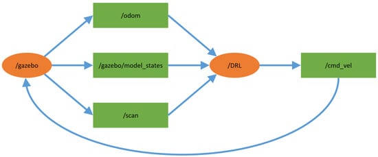
Figure 1.
The practical topology used in the experiments.
Next, according to above-mentioned simulation environment information, sends the action instructions based on the control strategy of the corresponding DRL method as feedback to via the topic . Finally, operates the UGV and updates all the states of the UGV and the simulation environment. Again, based on the ROS architecture, for the applications of different DRL approaches (DDPG and DQN), it only needs to replace the source code in with another example.
The design of the reward mechanism is divided into the following three parts:
- Non-collision;
- Collision;
- Reaching the goal.
Obviously, for the states of collision and reaching the goal, the current procedure will be terminated. The state of non-collision is formulated as shown below:
where C is a factor chosen empirically according to the simulation settings, is the distance between the goal and the UGV, defined as
and is the angle difference between the goal and the UGV, given by
in which is the movement around the yaw axis of the UGV and can be calculated as:
Note that the main concepts of the reward architecture in Equation (3) are:
- : Putting in the denominator means that getting closer to the goal will result in a higher reward;
- : Subtracting means that facing the goal will result in a higher reward;
- C: A factor that should be determined empirically. For different settings, different values of C may induce different performances. In the simulation, .
Since the action space of DQN is discrete, the action mechanism devised for the UGV in the experiments includes fewer action types, e.g., the rotation mode is simulated with fixed states. On the other hand, the action space of DDPG is continuous, and the action mechanism devised for the UGV in the experiments includes more/continuous/infinite action types in the simulation. For example, the rotation of the UGV can occur through any rotation angle within the specific rotation velocity.
For the design of the action mechanism, there are two independent designs for DDPG and DQN. First, for DQN, the moving velocity is fixed at 0.15 m/s. Then, in Figure 2, there are two kinds of rotation modes, as shown below:
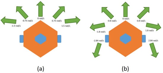
Figure 2.
Two kinds of rotation modes for DQN: (a) 5 states and (b) 7 states.
- With five states: rad/s, rad/s, 0 rad/s, 0.75 rad/s, and 1.5 rad/s;
- With seven states: rad/s, rad/s, rad/s, 0 rad/s, 0.8 rad/s, 1.8 rad/s, and 2.84 rad/s.
For DDPG, since it can adapt to an environment with a continuous action space, the range of moving velocity is set to 0∼0.22 m/s and the rotation velocity is set to ∼2.5 rad/s.
Moreover, a decaying exploration is used. This is then utilized as the scale of the normal distribution on the action sets obtained from the DDPG and DQN models, for the next action and future training procedures.
4. Experimental Results
In the simulation study, the Gazebo simulator of ROS was used to realize and verify the DRL methods. Furthermore, the TurtleBot3 model of Gazebo was also utilized in the experiments. During the process, Gazebo continuously updates all environment information, including the current position of TurtleBot3, the pose and the current position accumulated by the odometer, the information of the simulation environment scanned by the lidar sensor mounted on TurtleBot3, and so on, while TurtleBot3 interacts with the environment.
For the simulation scenarios, two kinds of environments are shown in Figure 3 and Figure 4, and the comparison between the two scenarios is presented in Table 1. The settings were as follows:
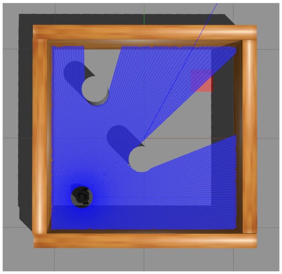
Figure 3.
The first experimental scenario with larger size and two obstacles.
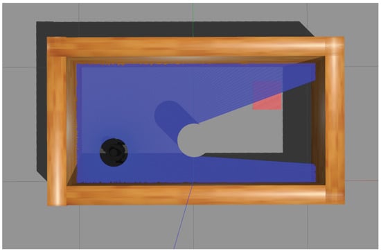
Figure 4.
The second experimental scenario with smaller size and one obstacle.

Table 1.
The comparison between the two scenarios.
- The sizes were and , respectively;
- The initial positions were and ;
- The goals (marked with red) were located at and ;
- There were two and one obstacles placed in each scenario, located at , , and ;
- The unit of all values presented above was meters;
- Three learning approaches, DQN with five states, DQN with seven states, and DDPG were considered in the simulation;
- Each procedure with the corresponding settings was executed 50,000 times;
- A decaying exploration was also utilized, which started from 1 and was multiplied by 0.9999 every five actions taken by the agent, after 50,000 actions were achieved;
- The specifications of the experimental computer were: CPU: Intel Core i7-10750H; RAM: 40 GB DDR4 2666 MHz, and GPU: Nvidia GeForce RTX 2070 GDDR6 8 GB.
First, the statistics of two scenarios are shown in Table 2 and Table 3, where the information regarding the smallest number of steps to reach the goal of each simulation and the corresponding training time (round) is gathered. Note that a learning procedure for a setting was executed 50,000 times (50,000 rounds) and could be terminated due to the events of a collision or reaching the goal. For example, for the setting of DQN with five states in the first scenario, the UGV only required 63 steps to reach the goal in the 23,167th round. This is the best record for the setting of DQN with five states in the first scenario. According to the statistics, DDPG had the best performance in two scenarios. The secondbest performance was obtained from DQN with seven states, and the worst with DQN with five states. Hence, if a control strategy has more action states to choose, it shows better performance in controlling the UGV, i.e., fewer steps to reach the goal and less training time to find the smallest number of steps for reaching the goal.
Table 2.
The statistics for the first scenario, including smallest number of steps to reach the goal and the training time required to find the smallest number of steps for reaching the goal.
Table 3.
The statistics for the second scenario, including the smallest number of steps to reach the goal and the training time required to find the smallest number of steps for reaching the goal.
For a more complex scenario, i.e., the first scenario, there is a larger gap in performance between DQN with seven states and DQN with five states. However, for a simpler scenario, the gap between the above two approaches is smaller. In particular, the number of steps required to reach the goal is almost the same. Consequently, if the number of action states of a UGV is in direct proportion to the price of its hardware, cheaper hardware could be chosen for a simpler scenario, due to the gap in performance.
Note that in the above paragraphs, the units of the smallest time to reach the goal and training time are the number of steps and rounds rather than the clock time. The main purpose is to separate the estimation from computer performance. Hence, no matter what computer is used, the estimation presented in the above paragraphs remains constant.
Last but not least, Figure 5 and Figure 6 demonstrate the average rewards with respect to the corresponding control strategies for every 1000 UGV rides. Note that the reason for considering every 1000 rides is that doing so enables us to illustrate the results more clearly and readably. In accordance with the experimental results, at the beginning, since most rides are finished due to a collision event, the reward values are lower. Then, the proportions of non-collision events and instances of reaching the goal become higher, and the reward values also become higher. More importantly, the larger the adopted number of states, the lower the reward value at the beginning. This is reasonable, since there are more possibilities that must to be explored. Moreover, proceeding with the training procedures, the control strategy with a larger adopted number of states will finally reach a better performance. In particular, DDPG > DQN with seven states > DQN with five states.
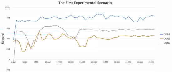
Figure 5.
The statistics of average rewards in the first experimental scenario.
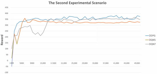
Figure 6.
The statistics of average rewards in the second experimental scenario.
5. Conclusions
In this paper, several control strategies were presented for the purpose of path planning and obstacle avoidance for UGVs. The goal was to find and discuss the optimal solution under different scenarios. In particular, the abilities of the control strategies were exhibited via several simulation experiments with various settings. According to the results, the learning processes achieved more accurate results with more adopted states and actions.
Furthermore, there was no learning approach that always possessed the best performance in all respects. For example, although more adopted states and actions led to more accurate results, more expensive hardware with higher performance was needed to support the procedure. Consequently, in the future, a challenge will be to combine DRL methods to integrate their learning procedures/structures for taking better decisions for all the different experiments, considering, e.g., hardware performance/price, sensor performance/price, and so on. There is a trade-off between accurate performance and reasonable cost. This is one of the most difficult issues.
However, some applications may have more robots in the same scenario simultaneously. Hence, realizing path planning and obstacle avoidance and interacting with other UGVs in the same scenario simultaneously by utilizing multi-agent deep reinforcement learning is also an important and interesting problem.
Lastly, the concept of reinforcement learning requires many trial-and-error searches. It is hard, or even impossible, to realize this directly via an experiment in a real environment. Hence, simulation is needed to derive a better algorithm first, and then port the training results to the real machine. Obviously, in the porting step, adjustments are still necessary. This is also a critical topic.
Author Contributions
Conceptualization, J.T. and C.-C.C.; methodology, J.T. and C.-C.C.; software, Y.-C.O. and B.-H.S.; validation, C.-C.C., B.-H.S., and Y.-M.O.; formal analysis, C.-C.C., B.-H.S., and Y.-M.O.; writing—original draft preparation, J.T. and C.-C.C.; writing—review and editing, J.T. and C.-C.C. All authors have read and agreed to the published version of the manuscript.
Funding
This research was supported by the Ministry of Science and Technology, Taiwan, R.O.C., under grants 110-2221-E-005-017-, 109-2221-E-035-067-MY3, and 109-2622-H-035-001-.
Institutional Review Board Statement
Not applicable.
Informed Consent Statement
Not applicable.
Data Availability Statement
Not applicable.
Conflicts of Interest
The authors declare no conflict of interest.
References
- Dionisio-Ortega, S.; Rojas-Perez, L.O.; Martinez-Carranza, J.; Cruz-Vega, I. A Deep Learning Approach towards Autonomous Flight in Forest Environments. In Proceedings of the 2018 International Conference on Electronics, Communications and Computers (CONIELECOMP), Cholula, Mexico, 21–23 February 2018; pp. 139–144. [Google Scholar]
- Maximov, V.; Tabarovsky, O. Survey of Accuracy Improvement Approaches for Tightly Coupled ToA/IMU Personal Indoor Navigation System. In Proceedings of the International Conference on Indoor Positioning and Indoor Navigation, Montbeliard, France, 28–31 October 2013. [Google Scholar]
- Chang, C.-C.; Tsai, J.; Lu, P.-C.; Lai, C.-A. Accuracy Improvement of Autonomous Straight Take-off, Flying Forward, and Landing of a Drone with Deep Reinforcement Learning. Int. J. Comput. Intell. Syst. 2020, 13, 914–919. [Google Scholar] [CrossRef]
- Sutton, R.S.; Barto, A.G. Reinforcement Learning: An Introduction; The MIT Press: Cambridge, MA, USA, 2018. [Google Scholar]
- Sewak, M. Deep Reinforcement Learning; Springer: Singapore, 2019. [Google Scholar]
- Francois-Lavet, V.; Henderson, P.; Islam, R.; Bellemare, M.G.; Pineau, J. An Introduction to Deep Reinforcement Learning. Found. Trends Mach. Learn. 2018, 11, 219–354. [Google Scholar] [CrossRef] [Green Version]
- Mishra, R.; Javed, A. ROS based service robot platform. In Proceedings of the 4th International Conference on Control, Automation and Robotics (ICCAR), Auckland, New Zealand, 20–23 April 2018; pp. 55–59. [Google Scholar]
- Quigley, M.; Conley, K.; Gerkey, B.; Faust, J.; Foote, T.; Leibs, J.; Wheeler, R.; Ng, A.-Y. ROS: An Open-Source Robot Operating System. ICRA Workshop Open Source Softw. 2009, 3, 5. [Google Scholar]
- Koenig, N.; Howard, A. Design and Use Paradigms for Gazebo, an Open-Source Multi-Robot Simulator. In Proceedings of the 2004 IEEE/RSJ International Conference on Intelligent Robots and Systems (IROS), Sendai, Japan, 28 September–2 October 2004; pp. 2149–2154. [Google Scholar]
- Chen, W.; Zhou, S.; Pan, Z.; Zheng, H.; Liu, Y. Mapless Collaborative Navigation for a Multi-Robot System Based on the Deep Reinforcement Learning. Appl. Sci. 2019, 9, 4198. [Google Scholar] [CrossRef] [Green Version]
- Feng, S.; Sebastian, B.; Ben-Tzvi, P. A Collision Avoidance Method Based on Deep Reinforcement Learning. Robotics 2021, 10, 73. [Google Scholar] [CrossRef]
- Zhu, P.; Dai, W.; Yao, W.; Ma, J.; Zeng, Z.; Lu, H. Multi-Robot Flocking Control Based on Deep Reinforcement Learning. IEEE Access 2020, 8, 150397–150406. [Google Scholar] [CrossRef]
- Chang, C.-C.; Tsai, J.; Lin, J.-H.; Ooi, Y.-M. Autonomous Driving Control Using the DDPG and RDPG Algorithms. Appl. Sci. 2021, 11, 10659. [Google Scholar] [CrossRef]
- Krishnan, S.; Boroujerdian, B.; Fu, W.; Faust, A.; Reddi, V.J. Air Learning: A Deep Reinforcement Learning Gym for Autonomous Aerial Robot Visual Navigation. Mach. Learn. 2021, 110, 2501–2540. [Google Scholar] [CrossRef]
- Shin, S.-Y.; Kang, Y.-W.; Kim, Y.-G. Obstacle Avoidance Drone by Deep Reinforcement Learning and Its Racing with Human Pilot. Appl. Sci. 2019, 9, 5571. [Google Scholar] [CrossRef] [Green Version]
- The Most Powerful Real-Time 3D Creation Platform—Unreal Engine. Available online: https://www.unrealengine.com/en-US/ (accessed on 6 July 2022).
- Home—AirSim. Available online: https://microsoft.github.io/AirSim/ (accessed on 6 July 2022).
- Stockman, G.; Shapiro, L.G. Computer Vision; Prentice Hall PTR: Hoboken, NJ, USA, 2001. [Google Scholar]
- ROS.org|Powering the World’s Robots. Available online: https://www.ros.org/ (accessed on 6 July 2022).
- Gazebo. Available online: http://gazebosim.org/ (accessed on 6 July 2022).
- Dong, J.; He, B. Novel Fuzzy PID-Type Iterative Learning Control for Quadrotor UAV. Sensors 2019, 19, 24. [Google Scholar] [CrossRef] [PubMed] [Green Version]
- Odry, A. An Open-Source Test Environment for Effective Development of MARG-Based Algorithms. Sensors 2021, 21, 1183. [Google Scholar] [CrossRef] [PubMed]
- TurtleBot3. Available online: https://emanual.robotis.com/docs/en/platform/turtlebot3/overview/ (accessed on 6 July 2022).
- Lillicrap, T.P.; Hunt, J.J.; Pritzel, A.; Heess, N.; Erez, T.; Tassa, Y.; Silver, D.; Wierstra, D. Continuous Control with Deep Reinforcement Learning. arXiv 2019, arXiv:1509.02971v6. [Google Scholar]
- Spinning Up Documentation. Available online: https://spinningup.openai.com/en/latest/index.html (accessed on 6 July 2022).
Publisher’s Note: MDPI stays neutral with regard to jurisdictional claims in published maps and institutional affiliations. |
© 2022 by the authors. Licensee MDPI, Basel, Switzerland. This article is an open access article distributed under the terms and conditions of the Creative Commons Attribution (CC BY) license (https://creativecommons.org/licenses/by/4.0/).