Determination of Johnson–Cook Material and Failure Model Constants for High-Tensile-Strength Tendon Steel in Post-Tensioned Concrete Members

Abstract

The estimation of damage in steel tendons is important for evaluating the remaining capacity of existing tensioned members. This research focuses on calculating Johnson–Cook (LC) model and damage parameters of high-strength steel material through quasi-static and dynamic uniaxial tests. Finite element analysis is used to replicate the experimental procedure, and through dynamic image correlation analysis, the numerical results accuracy is verified. In this investigation, it is found that the JC model can accurately replicate deformation and stress concentration under different strain rates and triaxiality conditions and, thus, can be used for fracture analysis of prestressed concrete members.

1. Introduction

Clear understanding of damage and deformation caused in high-strength steel tendons due to plastic deformation, strain rate and stress concentration effects is of critical importance for the accurate evaluation of existing tensioned concrete members. During regular operation and function of tensioned members, tendons should remain elastic or well within their serviceability state. Despite that, in recent history, due to corrosion, damage on tensioned members of bridge girders has been reported by several researchers [1,2,3,4,5,6]. Corrosion-induced failure of tendons is not thoroughly included in typical design practices of prestressed members and may cause the collapse of bridges in which they are most commonly installed. In current practice, manual inspection along the length of tendons where corrosion is suspected to have occurred is necessary. Corrosion of tendons in these applications commonly occurs due to two primarily two reasons. On the one hand, cracks are formed in surrounding concrete or due to the prestressed member being in close proximity to chloride-contaminated water. On the other hand, tendon rupture at inadequate grouting positions in the sheathing occurs due to the ingress of water from anchoring points. Once corrosion has occurred in a tendon, depending on the severity, it can cause significant reduction in the cross-sectional area of the member [7] and thus induce an unfavorable stress concentration condition. Furthermore, in cases of severe corrosion, the remaining cross-sectional area might be inefficient for bearing the imposed service dead loads and might yield or fracture (Figure 1). In the latter case, depending on the condition of the surrounding tendons, complete failure might occur if during fracture and dynamic loading, redistribution capacity of the remaining tendons is exceeded. That is why the investigation of fracture performance of high-strength tendons under high strain rates and stress concentration conditions is important to properly evaluate the remaining capacity of a tensioned member.

Once the state of corrosion in a tensioned member is verified, risk assessment analysis can be performed, and thus, the remaining capacity can be simulated with the aid of finite element (FE) tools. One of the most common tools used by researchers [8,9,10,11] to evaluate the performance and characteristics of metals under coupled stress and high strain-rate conditions is the Johnson–Cook (JC) material model with damage [12] and it is currently one of the most widely incorporated models in commercial FE software packages, due to its ability to predict material behavior with accuracy and speed, and because it couples a flow stress model with strain rates, elevated temperatures as well as stress concentration conditions.

K. Xu et al. [13] performed an experimental investigation of seven high-strength steels in an effort to propose a modification to the traditional JC constitutive model. In their research, BH300, HSLA350, 440 W, HSS590, TRIP590, DP600 and DP800 steel materials were used in uniaxial tensile tests with strain rates ranging from 0.005 s⁻¹ to 1000 s⁻¹, at normal environmental temperatures, as the heat-related material softening was not the primary objective of the research. Results were used to calibrate material parameters of the traditional JC constitutive model as well as for the evaluation of resulting differences between their proposed model, the traditional JC model, and the experimental data. From their research, it was found that from strain ranges of 2–15% and a tensile strength of 450–850 MPa, the proposed model had an average error of 2%, which is acceptable.

K. Vedantam et al. [14] investigated the mechanical response of two types of steel, Mild and DP590, in tension, at room temperature, using quasi-static and split Hopkinson bar techniques at strain rates ranging from 0.001 s⁻¹ to 1800 s⁻¹, and the resulting data were used to calculate the JC model parameters. It was found that for increasing strain rates, fracture strain as well as ultimate stress values increased in a similar manner approaching ultimate stress values of 1000 MPa. Finally, detailed JC material parameters were presented.

From the performed literature investigation, it was clearly identified that to accurately model the fracture behavior of high-strength steels, proper material definition and model calibration is required. The data necessary for the aforementioned FE modeling need to be obtained through expensive and time-consuming experimental effort under both high strain rates and high-stress concentration conditions to accurately consider both damage initiation and progression parameters. For high-tensile-strength tendon material commonly used in Japanese infrastructure in general, readily available model constants are not available. In this work the overall behavior, including plastic deformation and the fracture characteristics of medium-carbon high-strength steel used in tensioned members, has been studied through extensive experimental analysis under quasi-static and medium strain-rate loading conditions as well as stress concentration through the implementation of the tensile testing of notched specimens. Failure parameters and material constants for the JC model under room temperature have been calculated through the analysis of experimental data. Damage growth parameters are also introduced and proposed for accurate modeling of necking and fracture of tensile specimens under uniaxial loading conditions. The constants have been evaluated through numerical modeling of dog-bone-type tensile specimens under uniaxial loading conditions for strain rates similar to the experimental configuration as well as implementing digital image correlation (DIC) for the verification of strain propagation during different strain-rate and stress concentration conditions.

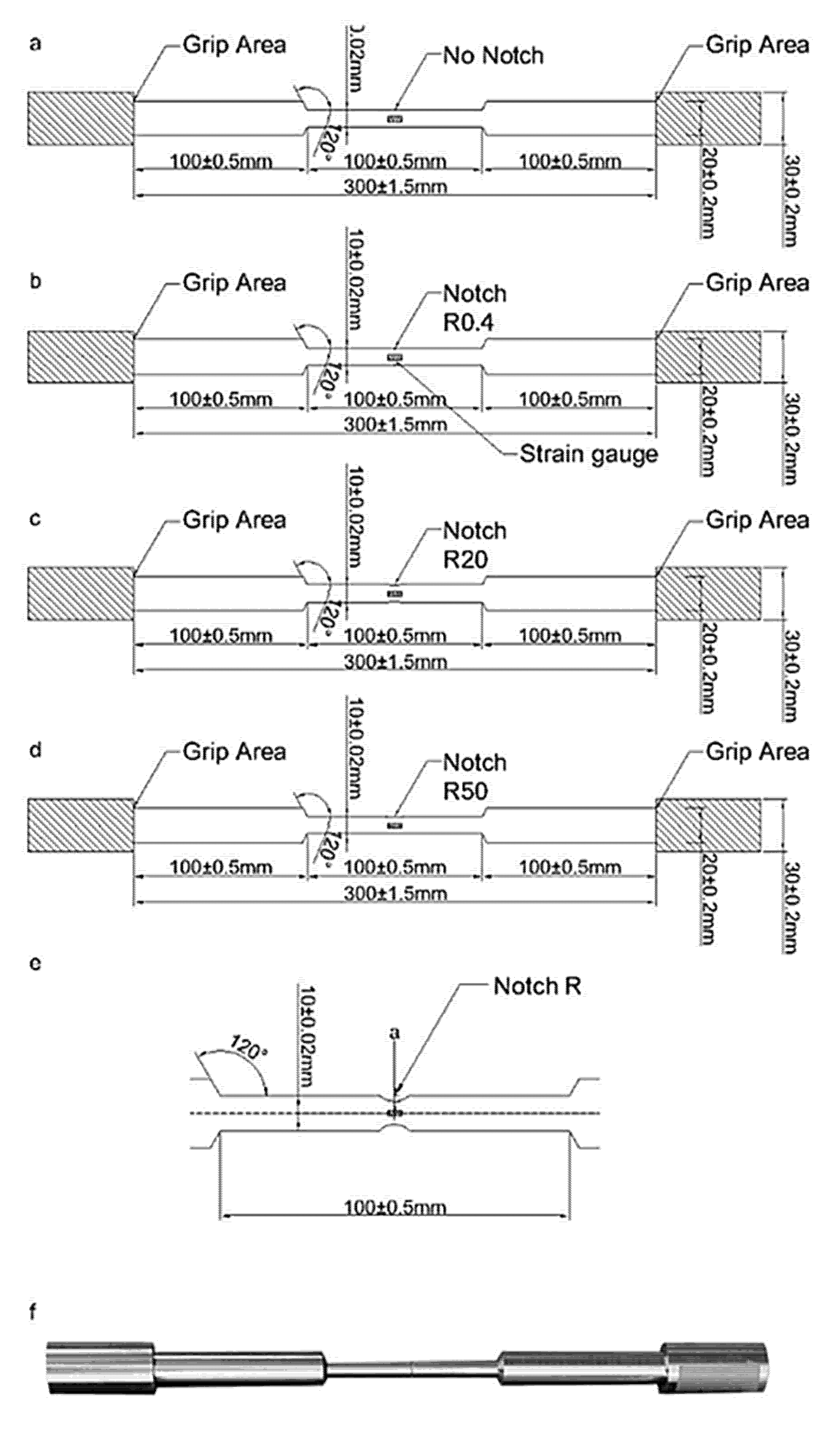
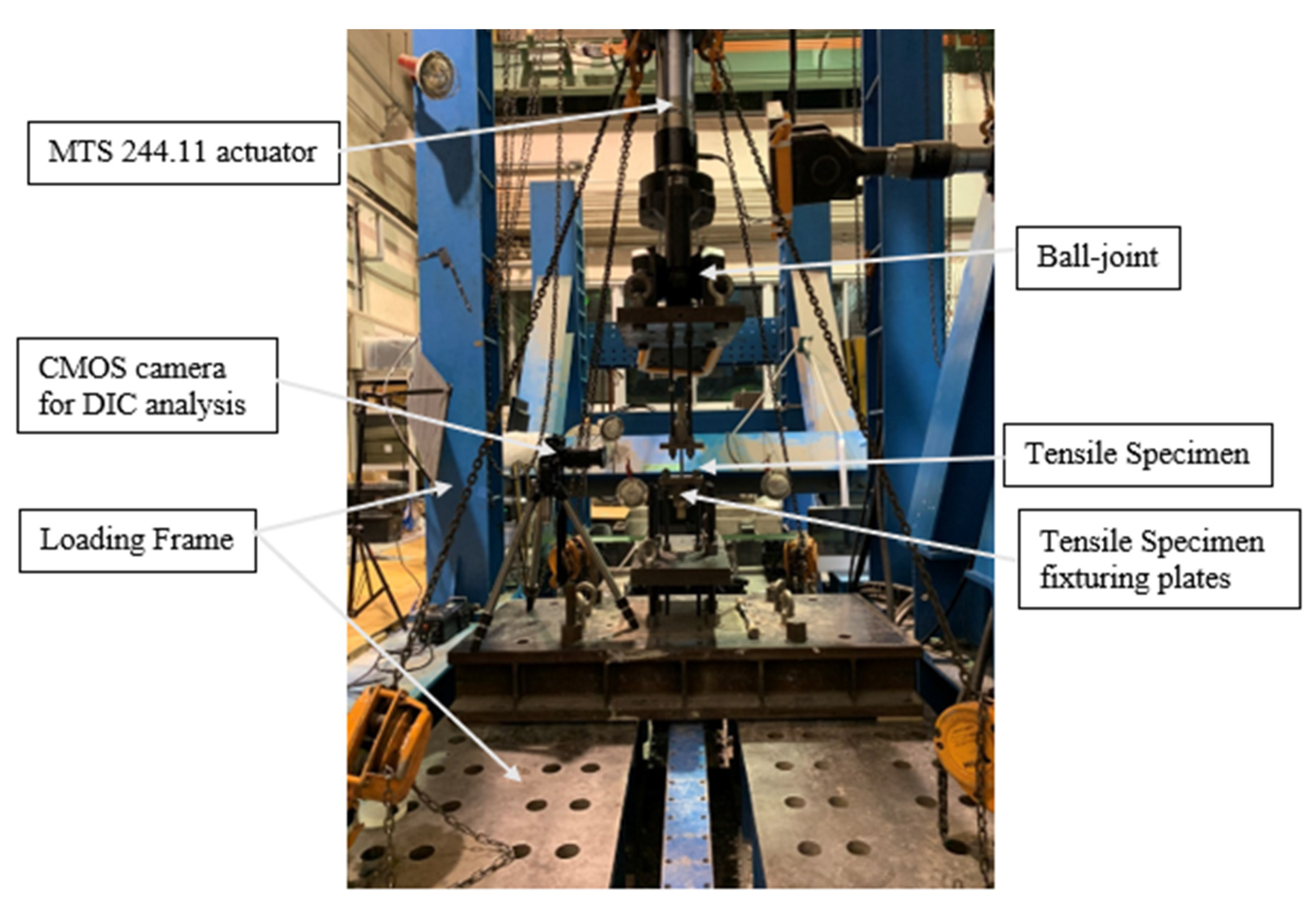
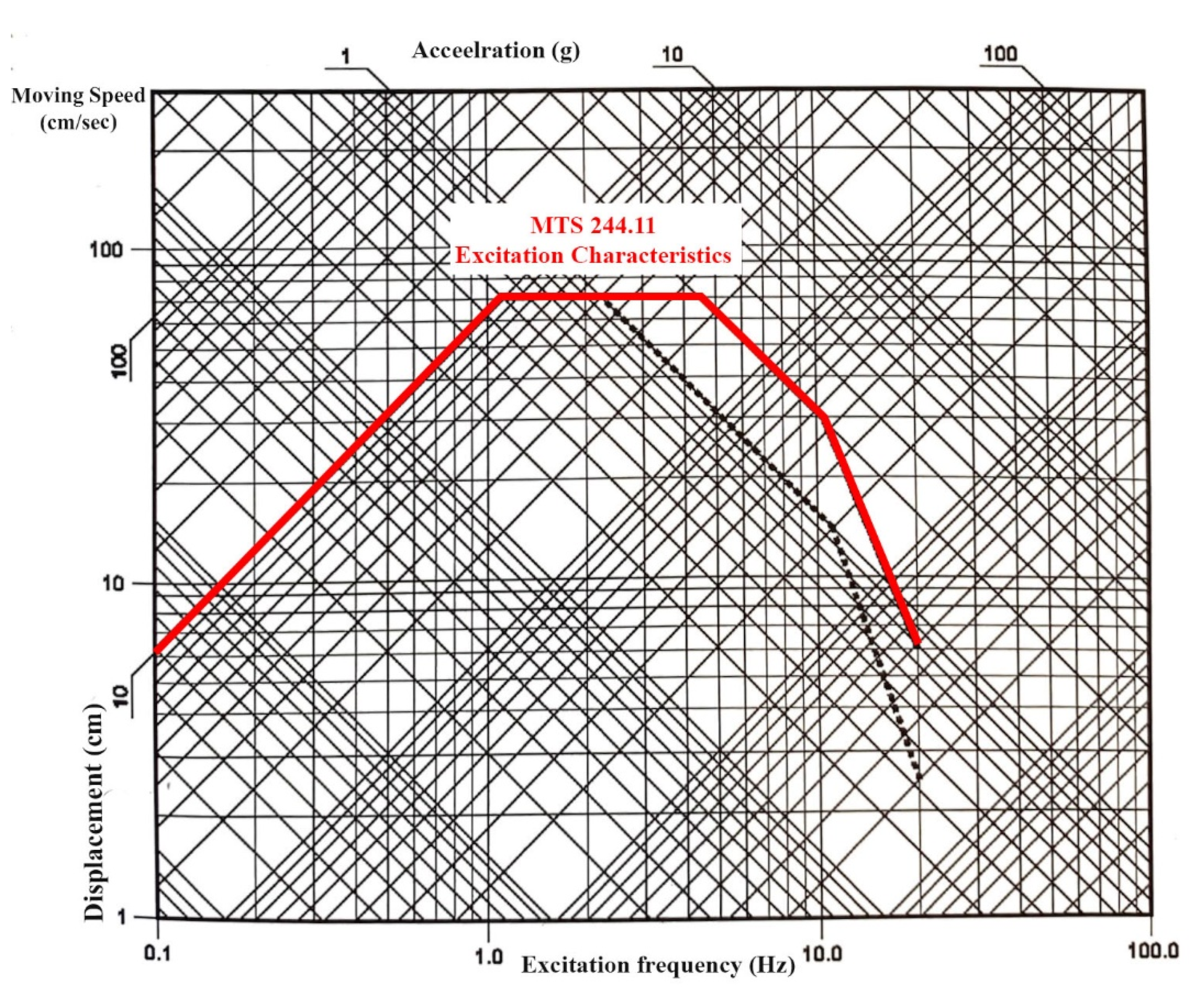
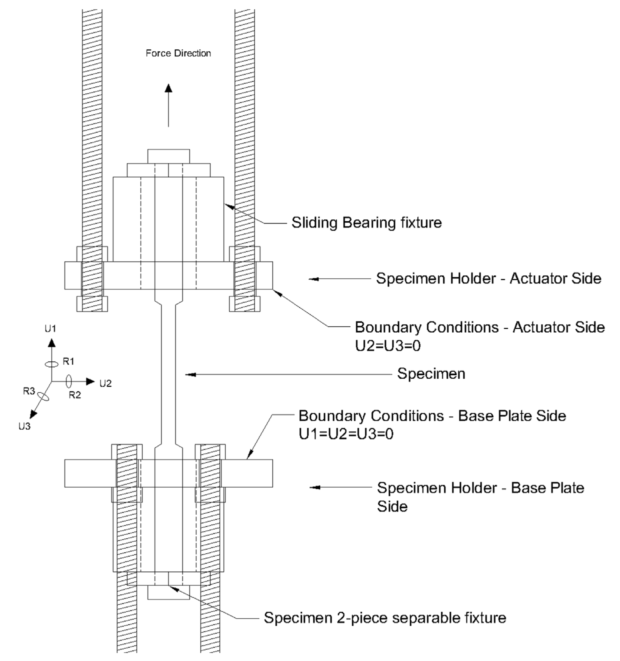
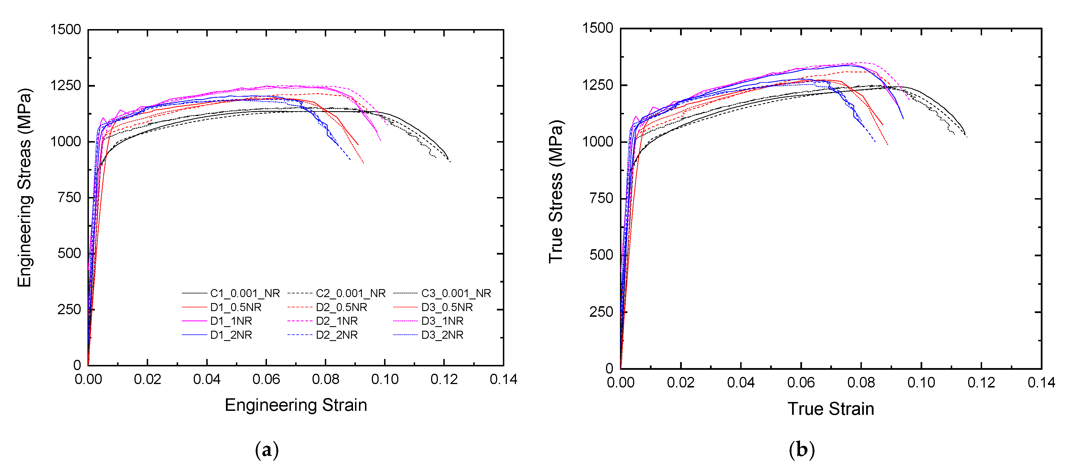
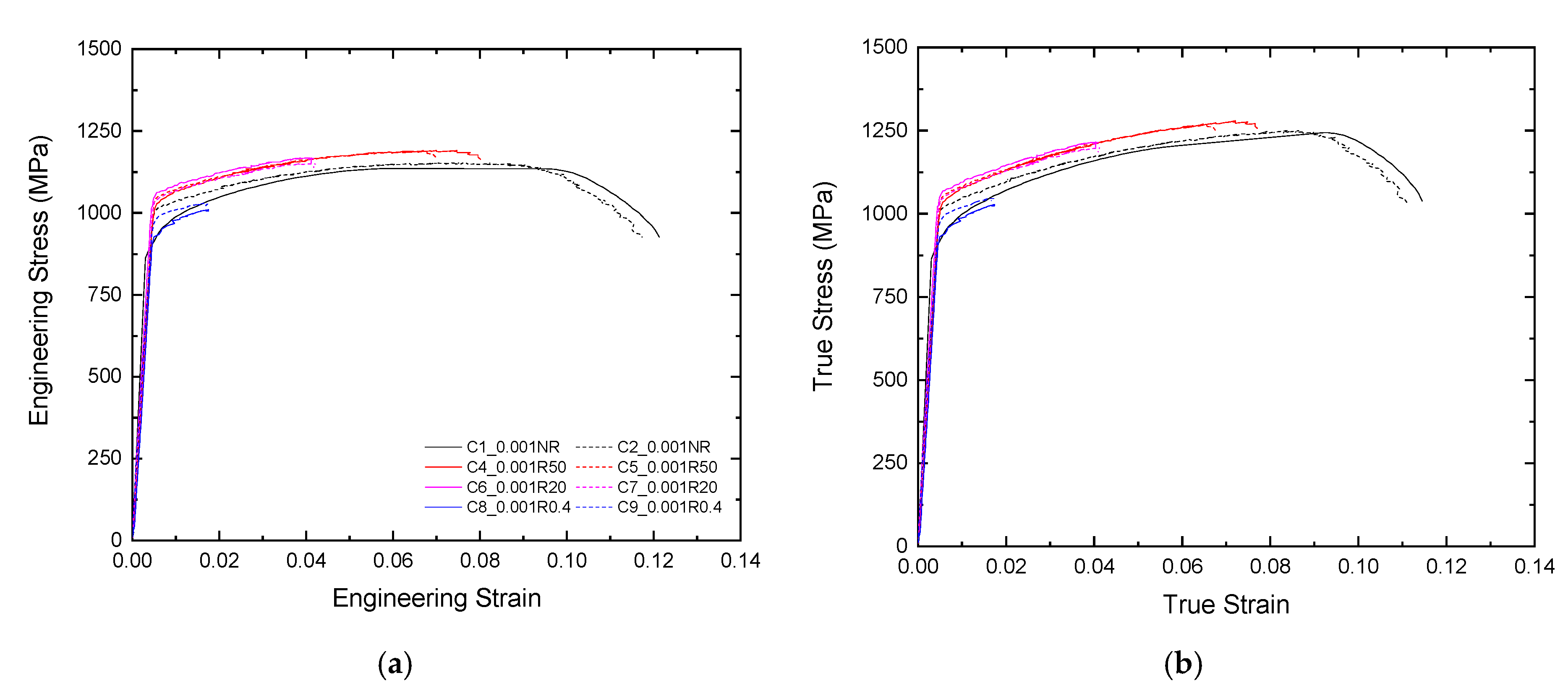
2. Materials and Experimental Procedure

In this research, the SBPR 930/1080 Type B No. 1 medium carbon high-strength steel was investigated, and its chemical composition is presented in

Table 1. Chemical composition of SBPR 930/1080 Type B No. 1 medium carbon steel (in wt%).

C	Si	Mn	P	S	Cu
0.60–0.65	0.12–0.32	0.30–0.60	≤0.030	≤0.035	≤0.30

(in wt%). The material used for the manufacturing of the specimens was supplied by a local company according to JIS G 3109 [15], in 450 mm × 32 mm cylindrical pieces out of which the dog-bone type specimens were manufactured using a manual lathe. Geometrical details can be seen in Figure 2, for cylindrical specimens used throughout this research for both quasi-static and dynamic tensile tests, with smooth as well as notched gauge lengths. For the tensile tests, MTS 244.11 servo-hydraulic actuator (Figure 3) was used. Acceleration, velocity, displacement, and excitation frequency characteristics are represented in Figure 4. Despite the dynamic characteristics of the experimental procedure, experimental parameters were well within the capability envelope of the utilized actuator. The actuator was mounted on a loading frame using ball-joints for both fixed and extendable part of the piston to allow for increased mobility and flexibility under various testing conditions and requirements. For this research, both specimens and actuator were positioned and fixed in a vertical orientation to ensure an inline application of pulling force (Figure 5).

Furthermore, to ensure constant pulling rate, the loading end of the specimens were constructed in such a way as to allow for initial retraction of the actuator’s piston without exerting force onto the specimen. Once required velocity is achieved, and after that stage, contact between the top of the specimen and the mounting fixture (plate) at the movable end of the actuator is initiated, transferring the resulting load onto the specimen body. As can be seen in

Table 2. Manufactured specimen specifications and testing parameters (C—static; D—dynamic _strain rate_notch radius).

Specimen Nomenclature	Testing Speed (mm/s)	Strain Rate during Tensile Test (s−1)	Specimen Type	Radius R (mm)	Minimum Radius A (mm)	${\mathit{\eta }}^{*}$
C1_0.001_NR	0.1	0.001	Smooth	-	-	0.333
C2_0.001_NR	0.1	0.001	Smooth	-	-	0.333
C3_0.001_NR	0.1	0.001	Smooth	-	-	0.033
D1_0.5NR	50	0.5	Smooth	-	-	0.333
D2_0.5NR	50	0.5	Smooth	-	-	0.333
D3_0.5NR	50	0.5	Smooth	-	-	0.033
D1_1NR	100	1	Smooth	-	-	0.333
D2_1NR	100	1	Smooth	-	-	0.333
D3_1NR	100	1	Smooth	-	-	0.033
D1_2NR	200	2	Smooth	-	-	0.333
D2_2NR	200	2	Smooth	-	-	0.333
D3_2NR	200	2	Smooth	-	-	0.033
C4_0.001R20	0.1	0.001	Notched	20	4.5	0.484
C5_0.001R20	0.1	0.001	Notched	20	4.48	0.484
C6_0.001R50	0.1	0.001	Notched	50	4.5	0.395
C7_0.001R50	0.1	0.001	Notched	50	4.48	0.394
C8_0.001R0.4	0.1	0.001	Notched	0.4	4	2.867
C9_0.001R0.4	0.1	0.001	Notched	0.4	3.98	2.961

, for dynamic loading cases, three specimens were tested for each required strain rate, and the resulting force-displacement data were converted into true stress–strain data using standard equations for uniaxial tensile tests. To further aid the calibration of the initial part of flow stress–strain curves, 2 mm strain gauges were attached using adhesive onto the specimens, and strain data were captured for values up to 20,000 μm, before the adhesive failure resulting in detachment of the strain gauges positioned in the middle of the respective gauge lengths.

From the flow stress–strain data of smooth (no notch) specimens (Figure 6a), it can be seen that for the same strain rate, similar stress–strain curves were obtained. For quasi-static strain rate (0.001 s⁻¹), this specific material showed the most ductile behavior fracturing, on average at 0.127 strain. In uniaxial dynamic tensile (Figure 6b) tests, it can be seen that for the case of 0.5 s⁻¹ strain rate, material showed a more brittle behavior while fracturing, on average at 0.092 strain. In comparison to the 0.5 s⁻¹ strain rate case, specimens tested at 1 s⁻¹ showed an increase in the ductility fracturing, on average at 0.099 strain, as well as showing the highest ultimate stress values overall. Finally, for the case of 2 s⁻¹ strain rate, specimens presented most brittle behavior out of all cases, while not showing any significant increase in their ultimate stress value when compared to the slowest dynamic case. In Figure 7, engineering stress–strain (initial cross-sectional area is used for the strain calculations) and converted true stress–strain (strain calculations are performed based on the actual cross-sectional area, which changes with time) data can be seen for quasi-static testing of notched specimens listed in Table 2. Similarly to the case of variable strain rate data, in the case of changing the notch size and radius, good agreement is observed between similar cases. Smooth specimens were the most ductile, and the fracture strain progressively reduced as the minimum specimen radius and notch radius decreased.

Notable reduction in both ultimate stress and failure strain for the C7_0.001R0.4 and C8_0.001R0.4, was observed, resulting in a considerably brittle fracture behavior in comparison to the smooth cases.

3. Johnson–Cook Model

The Johnson–Cook model is able to accurately analyze and predict stress–strain behavior for ductile materials, and its applicability as well as accuracy has been studied thoroughly in the literature for steel or aluminum alloys under combined conditions of large deformation, high strain rate as well as elevated temperatures focusing on metal forming or impact performance [16,17,18,19]. The JC stress model is expressed in Equation (1).

$$\sigma =\left(A+B{\epsilon }^n\right)\left(1+C\ln {\dot{\epsilon }}^{\ast }\right)(1-T^{{\ast }^m})$$

(1)

in which $\sigma$ represents von Mises or equivalent stress, A is the yield stress of tested material under reference conditions (strain rate and temperature), B is the strain hardening constant, n is the strain hardening coefficient, C is a coefficient of strain rate resulting in post-yield strengthening of the material, ${\dot{\epsilon }}^{\ast }$ is the dimensionless strain rate, $T^{\ast }$ homologous temperature, and m is a thermal softening coefficient. It can be observed that the JC model can be separated into three factors based on the static stress condition, influence of strain rate and, finally, influence of temperature when looking at the three parentheses from left to right. In Equation (1), the ${\dot{\epsilon }}^{\ast }$ parameter as well as $T^{\ast }$ can be defined in Equations (2) and (3).

$${\dot{\epsilon }}^{\ast }=\frac{{\dot{\epsilon }}_p}{{\dot{\epsilon }}_0}$$

(2)

$$T^{\ast }=\frac{T-T_{ref}}{T_m-T_{ref}}$$

(3)

where ${\dot{\epsilon }}_p$ is the accumulated plastic strain and ${\dot{\epsilon }}_0$ is the reference strain rate which, in this work, was taken as 0.001 s⁻¹. T_m is defined as the melting temperature of the material and T_ref is the reference temperature. For the scope of this research, performance of the high-strength medium carbon steel material was investigated under quasi-static and medium dynamic strain rates as well as varying stress concentration conditions, but the temperature factor was not considered since the primary failure factor of tensioned members is usually due to corrosion, as mentioned in previous sections.

3.1. Determination of Material Constants A, B, n

For ${\dot{\epsilon }}_p={\dot{\epsilon }}_0$ and $T=T_{ref}$ in Equation (1), the second and third parentheses are omitted, since the effects of strain rate strengthening and thermal softening are neglected. Modifying the remaining terms by taking the natural logarithm on both sides and using the averaged true stress–strain data from cases C1_0.001_NR, C2_0.001_NR and C3_0.001NR and linearly plotting the $\ln \left(\sigma -A\right)$ term with  of Equation (4), a linear regression model was used to fit the data points, as can be seen in Figure 8.

$$\ln \left(\sigma -A\right)=n\ln \epsilon +\ln B$$

(4)

The A parameter was also calculated under reference strain conditions using the 0.2% offset method. For the linear fitting presented in Figure 8, an R² factor of more than 97.5% was achieved, resulting in a good accuracy of the regression model. As a result of the latter, material constants A, B and n were calculated from the slope and intercept of the curve, which can be seen in

Table 3. Johnson–Cook material model parameters for SBPR 930/1080 Type B No. 1.

A (MPa)	B (Mpa)	C	n
933	1295	0.0221	0.5376

.

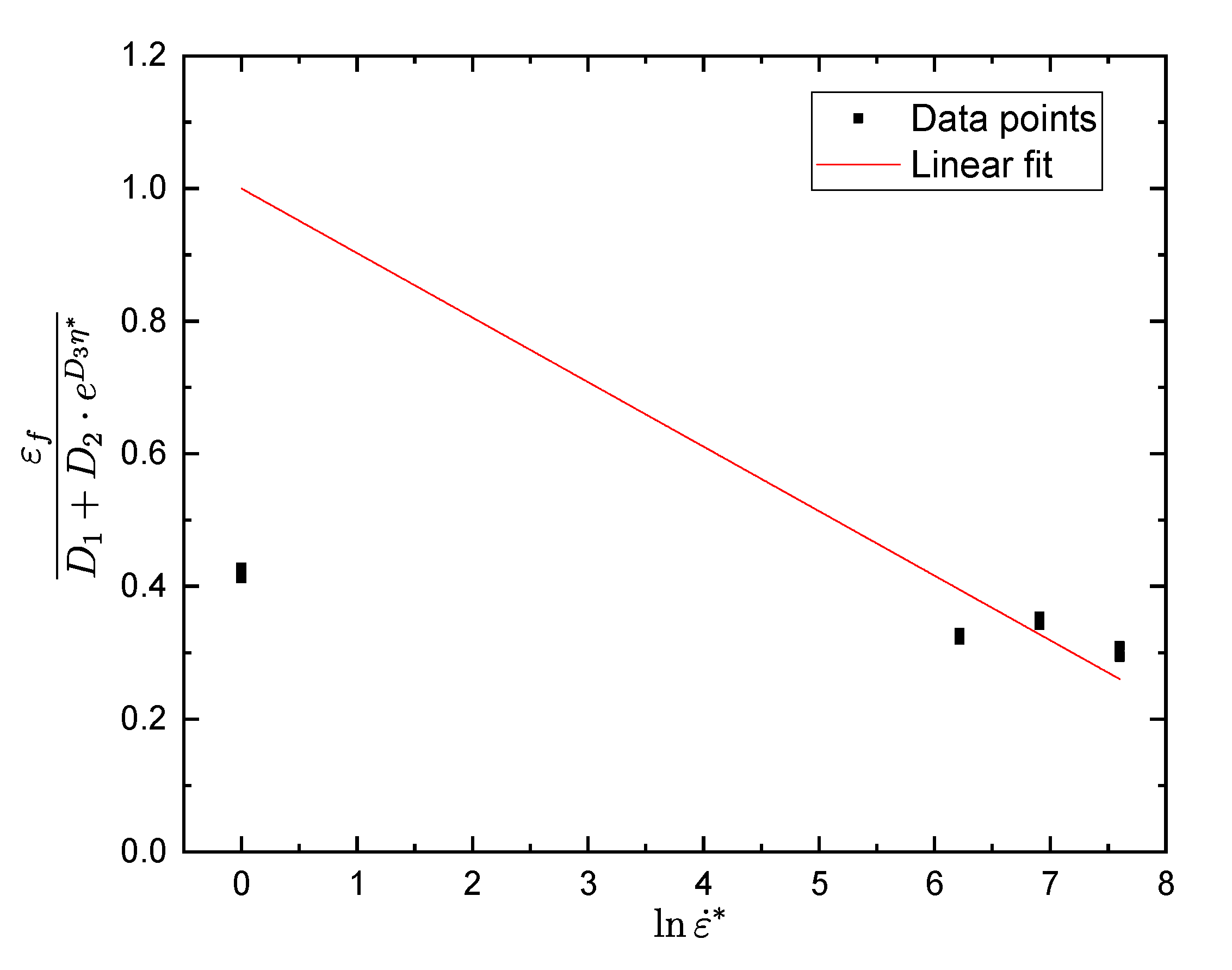
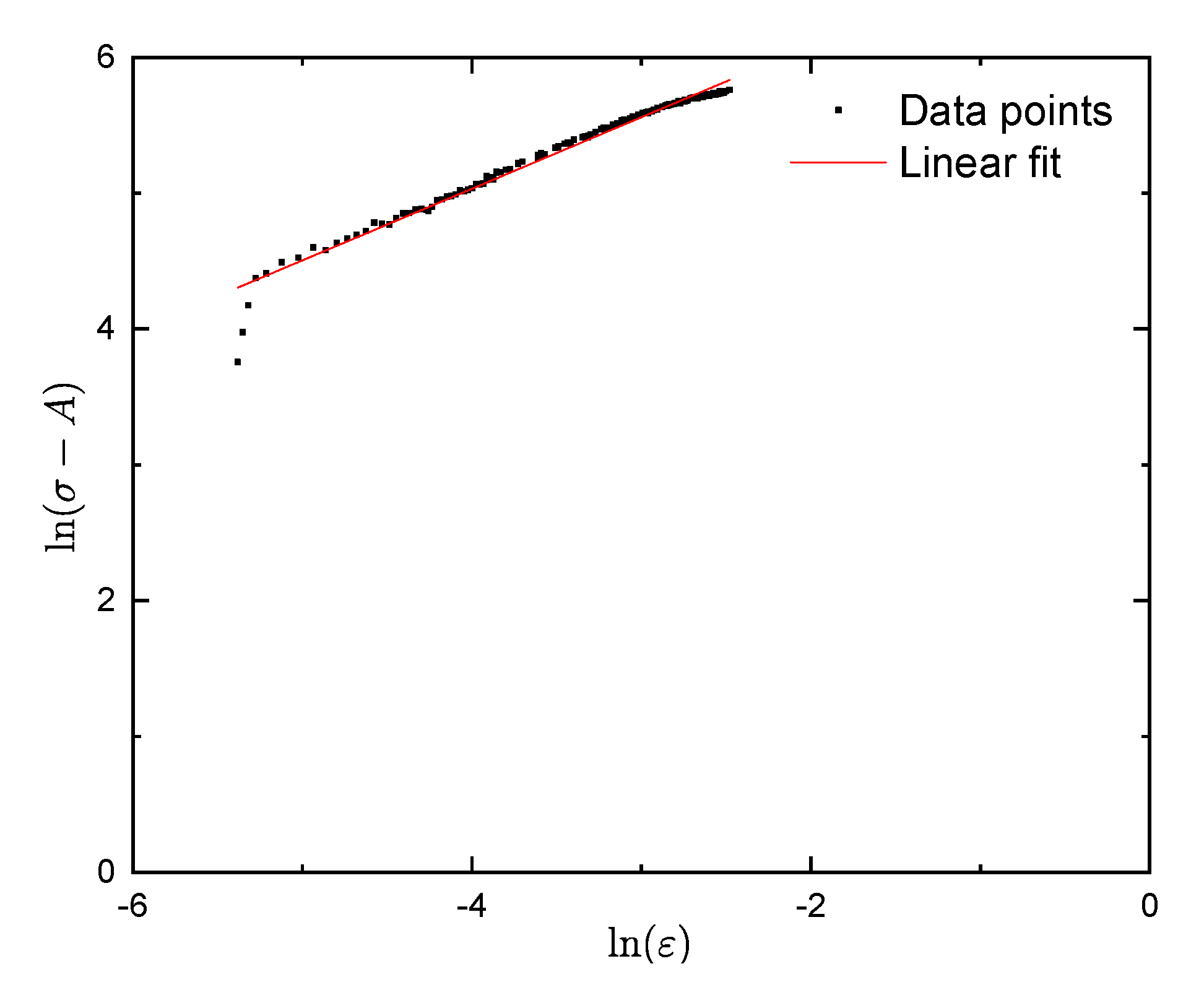
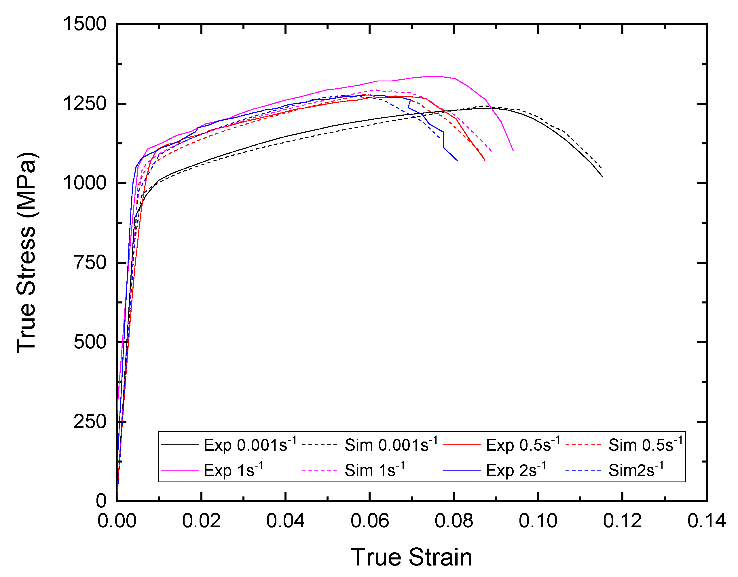
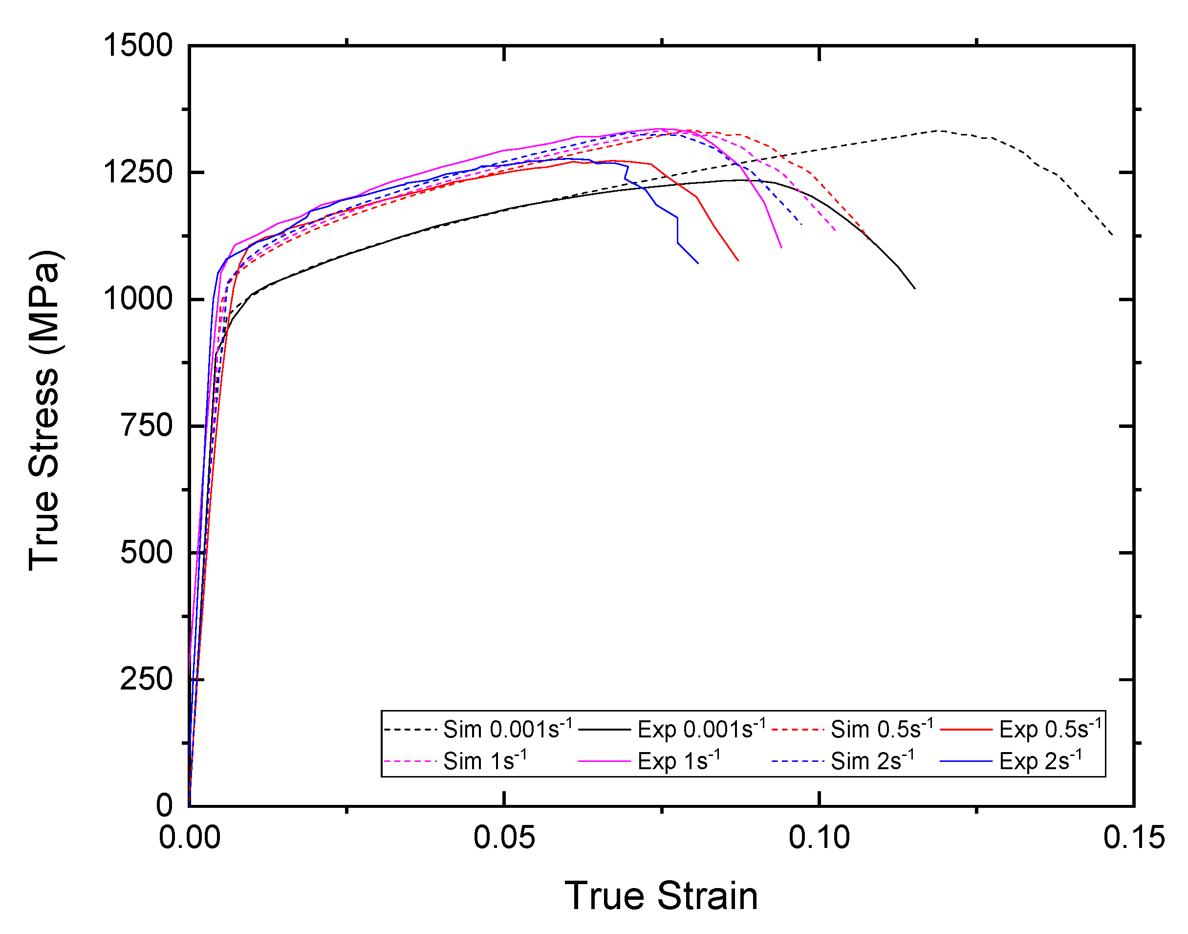
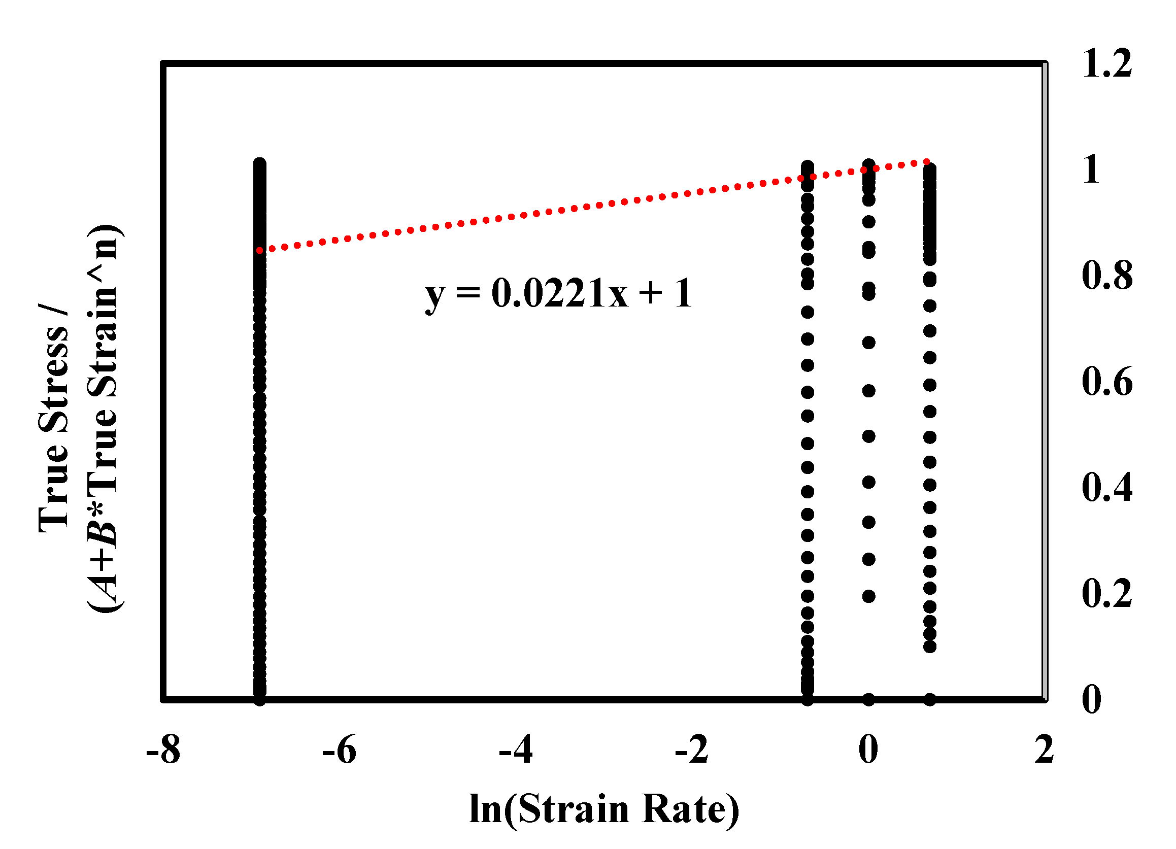
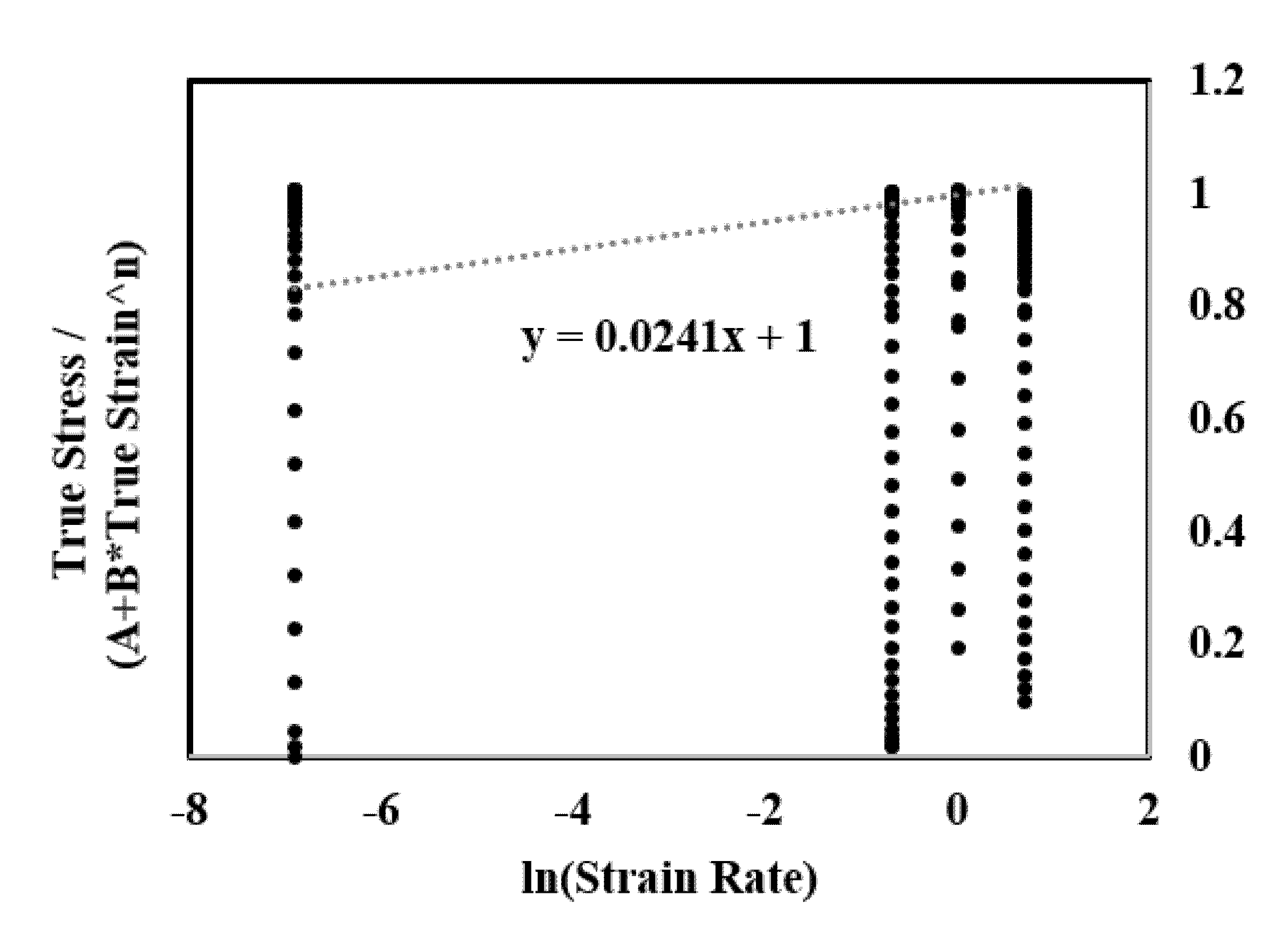
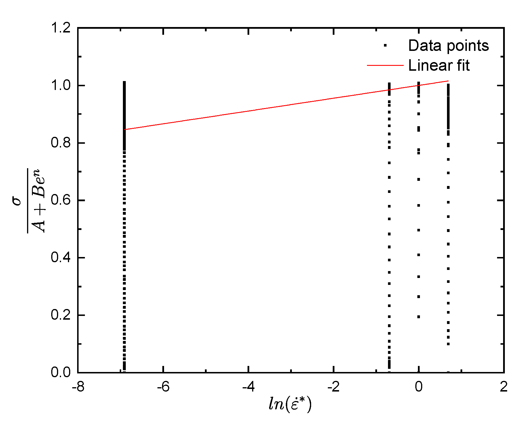
3.2. Determination of Material Constant C

For the purpose of this work and while not considering thermal softening effects, Equation (1) can be modified as:

$$\frac{\sigma }{\left(A+B{\epsilon }^n\right)}=\left(1+C\ln {\dot{\epsilon }}^{\ast }\right)$$

(5)

To obtain the C parameter, stress–strain data at four different strain rates (0.001 s⁻¹, 0.5 s⁻¹, 1 s⁻¹, 2 s⁻¹) were used to plot Figure 9, while utilizing A, B, n constants that were calculated in the previous section and substituted in Equation (5). Afterwards, first-order linear fitting was performed using a vertical axis intercept value of 1, since Equation (1) is in the form of $y=a+bx$ (C parameter’s calculation sensitivity analysis is presented in Appendix B). Similarly to Figure 8, from the slope of the linear regression fit, the C parameter was calculated, which can also be seen in Table 3.

The material constants that were calculated from the aforementioned constitutive equations for the JC model are summarized in Table 3.

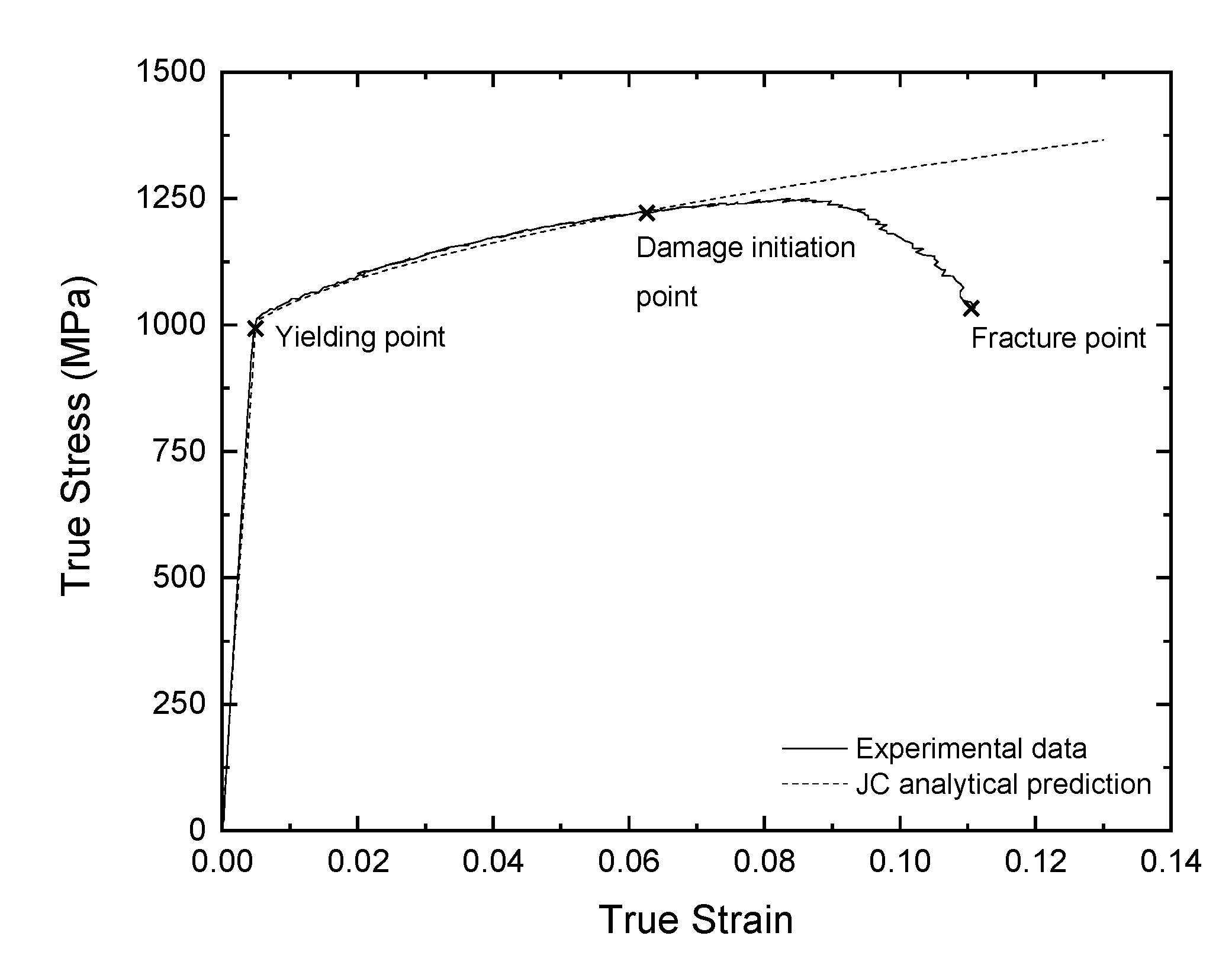
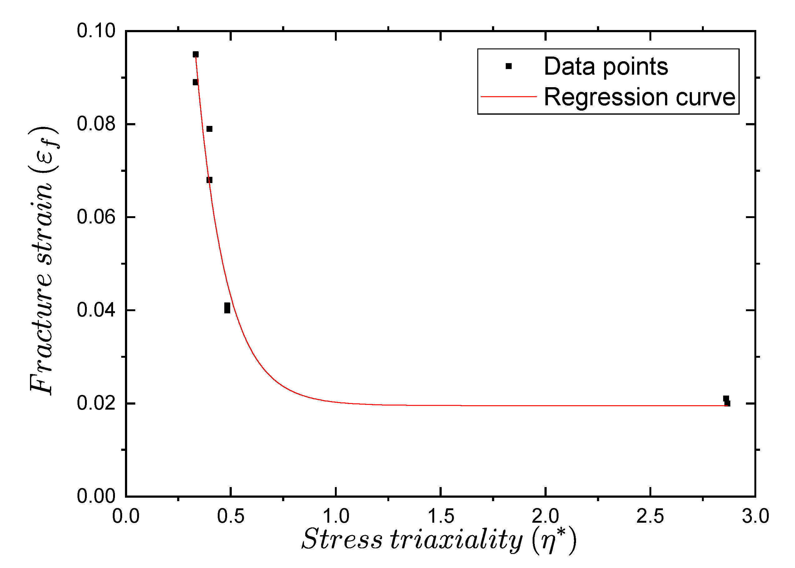
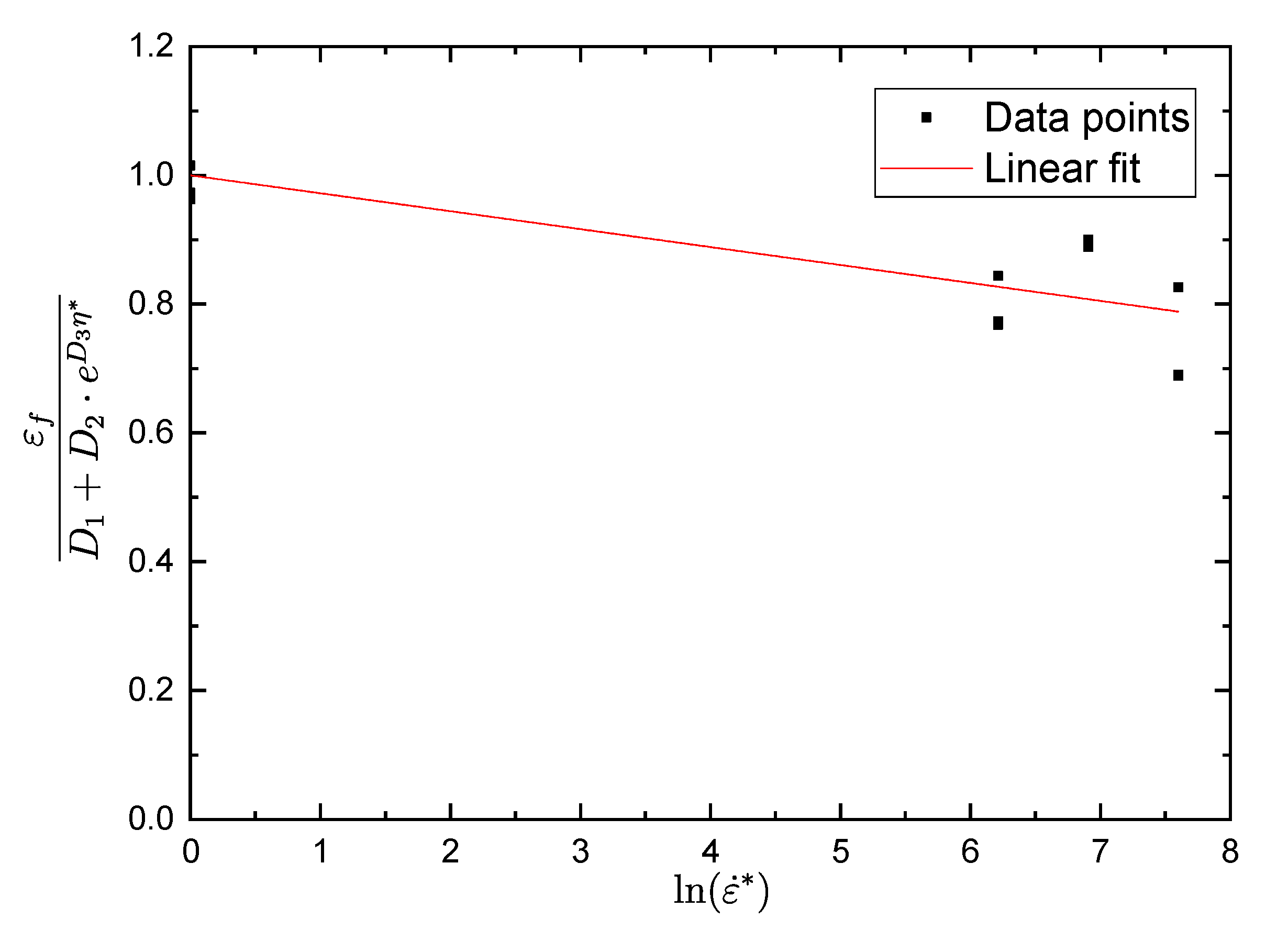
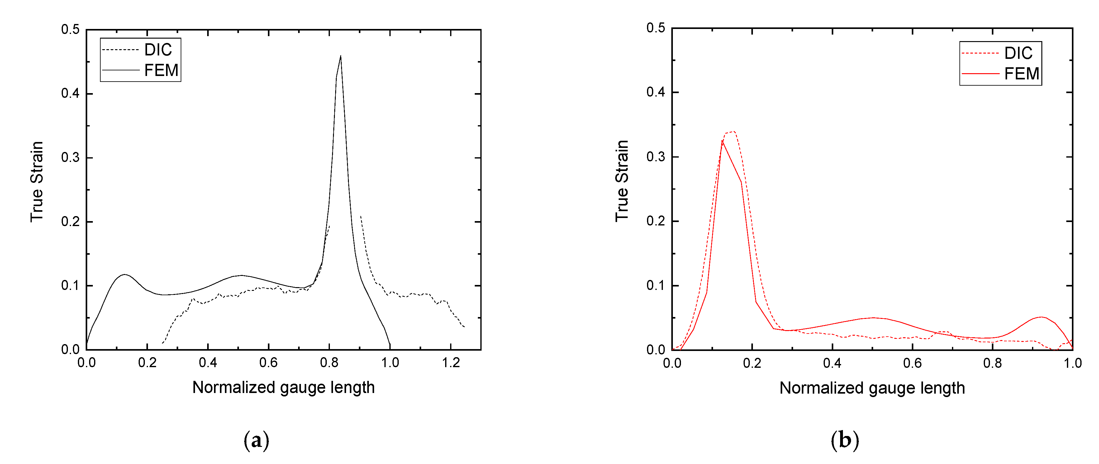
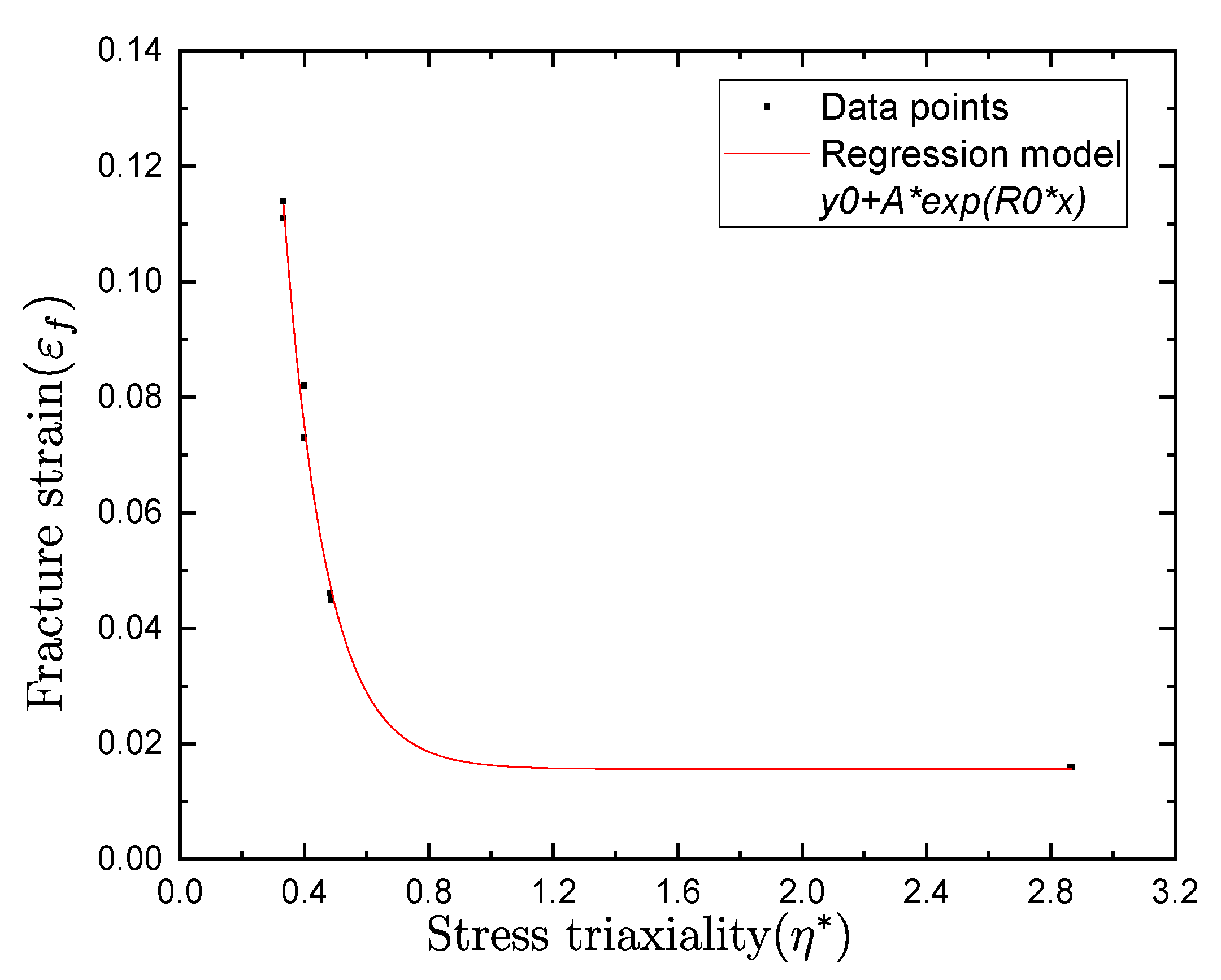
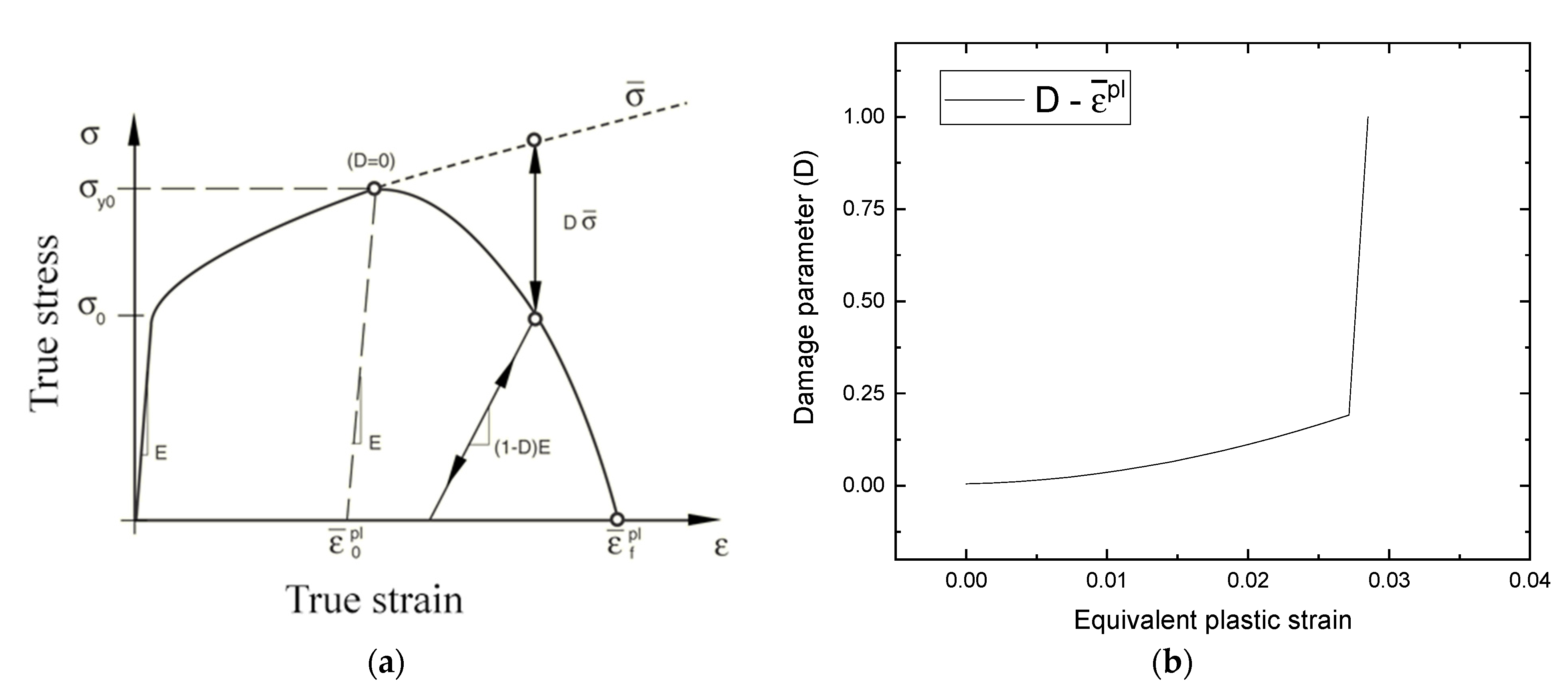
3.3. Johnson–Cook Damage Model Parameters

Substituting the material constants from Table 3 into Equation (1), the following relationships can be formed according to the JC model for stress, strain and strain deformation rate, as can be seen in Equation (6). When comparing experimental data with analytical prediction from Equation (6), good accuracy can be observed until the onset of damage and necking of the tensile specimen (Figure 10).

$${\sigma }_y=\left(933+1295{\epsilon }^{0.5376}\right)\left(1+0.0221\ln \left(\frac{{\dot{\epsilon }}^{\ast }}{0.001}\right)\right)\hspace{0.17em}\left(MPa\right)$$

(6)

To accurately simulate damage that occurs in the material model with regard to the JC damage parameter setting, it is important to define at which point damage is calculated. In this study, after careful consideration (Appendix A), the authors decided to use the Damage Initiation point of Figure 10. With that, the JC damage model is used to relate fracture strain with stress triaxiality ratio, strain rate as well as temperature [11,20], and it is expressed in Equation (7).

$${\epsilon }_f=\left(D_1+D_2{e}^{D_3\left(\frac{{\sigma }_m}{{\sigma }_{eq}}\right)}\right)\left(1+D_4\ln \left({\dot{\epsilon }}_p{}^{*}\right)\right)\left(1+D_5{T}^{*}\right)$$

(7)

D₁ to D₅ represent damage constants for the JC model, ${\sigma }_m$ is the mean stress (hydrostatic) and ${\sigma }_{eq}$ is the equivalent stress (von Mises). As damage occurs in an element governed by JC damage model, it is accumulated based on a damage law and can be represented by Equation (8) [21]. When damage occurs, during high levels of deformation, material strength is reduced [11] and the resulting relation for stress during this damage evolution step is presented in Equation (9).

$$D={\displaystyle \sum _{}^{}\left(\frac{\mathsf{\Delta }\epsilon }{{\epsilon }_f}\right)}$$

(8)

where $\mathsf{\Delta }\epsilon$ is the equivalent plastic strain increment and ${\epsilon }_f$ is the equivalent strain to fracture under certain stress, strain rate and temperature conditions.

$${\sigma }_D=\left(1-D\right){\sigma }_{eq}$$

(9)

In Equation (9), ${\sigma }_D$ is the resulting stress after damage in an element has been initiated, and $D$ is a damage parameter with the following conditions $\left(0\le D\le 1\right)$. In Equation (7), $\frac{{\sigma }_m}{{\sigma }_{eq}}$ can also be defined as stress triaxiality ratio ${\eta }^{*}$ [22,23], and along with equivalent stress can be obtained from undamaged material, while considering plastic deformation up until the onset of necking. According to the work of Bridgman [24], stress triaxiality values can be estimated from uniaxial tests of round specimens according to the analytical model which is presented in Equation (10).

$${\eta }^{*}=\frac{1}{3}+\ln \left(1+\frac{\alpha }{2R}\right)$$

(10)

In the model, ${\eta }^{*}$ is the stress triaxiality state value, $R$ represents the radius of notch that the specimen is manufactured according to and $\alpha$ represents the minimum cross section’s radius. Triaxialities calculated according to Bridgman’s model for different notched specimens can be seen in Table 2.

Neglecting the effects of strain rate and temperature, Equation (7) can be simplified representing fracture strain in terms of the aforementioned D₁ to D₃ damage parameters and stress triaxiality ratio effects. When plotting the fracture strain–stress triaxiality ratio (Figure 11), experimental tension data [25] is used, with 0.001 s⁻¹ strain rate for smooth and notched specimens from Figure 7b and Table 2, in the form of $y=A+B\cdot \exp \left(R0\cdot x\right)$; D₁ to D₃ damage parameters can be calculated from the exponential coefficients of the equation similar in principal to the derivation of Equation (4). Afterwards, the $D_4$ strain-rate-dependent parameter was calculated by rewriting Equation (7) complete with the previously calculated D₁ to D₃ damage parameters according to Equation (11). In detail, when plotting $\frac{{\epsilon }_f}{D_1+D_2\cdot e^{D_3{\eta }^{*}}}$ against $1+D_4\cdot \ln {\dot{\epsilon }}^{*}$ (Figure 12) and using a linear regression fitting equation intercepting the vertical axis at a value of 1.0, from the slope of the resulting equation, the final JC damage parameter $D_4$ was calculated.

$$\frac{{\epsilon }_f}{D_1+D_2\cdot e^{D_3{\eta }^{*}}}=1+D_4\cdot \ln {\dot{\epsilon }}^{*}$$

(11)

The calculated JC damage model parameters can be seen summarized in

Table 4. Johnson–Cook damage model parameters for SBPR 930/1080 Type B No. 1.

D1	D2	D3	D4	D5
0.0165	0.6622	−6.4791	−0.0279	0

and can be used in FE software to simulate yield and fracture of high-strength tendons in prestressed concrete applications.

4. Numerical Simulation

The purpose of the numerical modeling was to verify the reproducibility of the experimental results in the commercially available finite element software Abaqus Explicit [26], as part of a broader research work aimed at modeling the dynamic fracture behavior of prestressed concrete members. To accurately reproduce the dynamic fracture effects of high-tensile-strength tendons, non-linear dynamic analysis was used throughout the simulation process of uniaxial tensile tests. Full-scale, three-dimensional models were created, accurately reproducing the geometrical properties of the constructed specimens shown in Figure 2. In both single element and full-scale analysis, geometric nonlinearity related effects were taken into account by using the “NLgeom” option available in Abaqus Explicit.

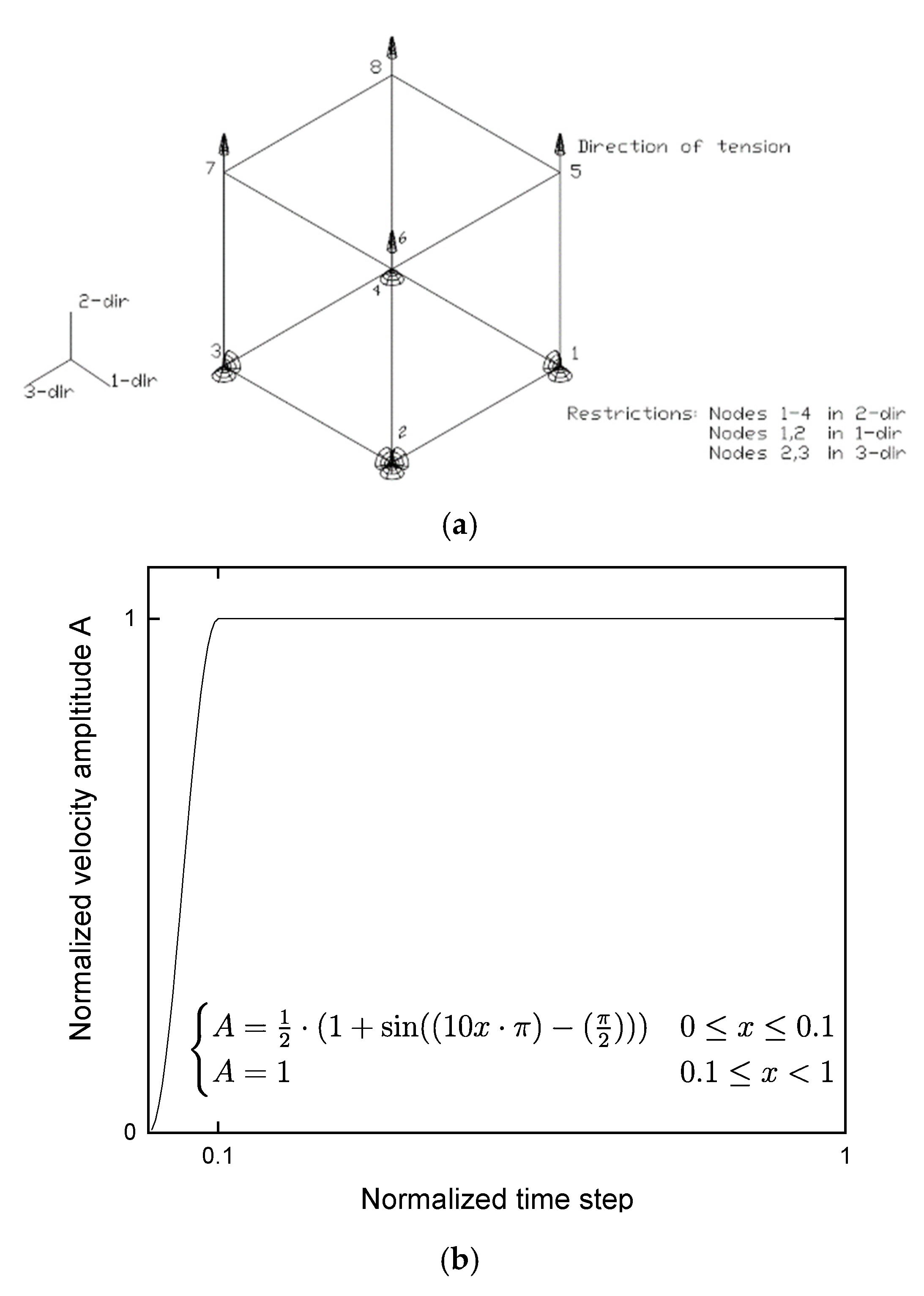
4.1. Numerical Simulation of Singular Finite Element

Initially, to verify the accuracy of the analytical model in FE simulations, a single 8-noded cubical-shaped C3D8R element measuring 1 mm³ was modeled, and suitable boundary conditions were applied to simulate biaxial symmetry in the two axes perpendicular to the loading direction. To maintain a stress triaxiality ratio ${\eta }^{*}$ of 0.333 throughout the tensile test, the bottom four nodes were restrained in the direction of applied force, and four nodes on each of the two faces perpendicular to the loading axis had their movement in the two orthogonal axes restrained, respectively, as can be seen in Figure 13a. The top four nodes were free to move in the direction of loading, and to achieve that a velocity-based loading condition was applied.

Similarly to the experimental procedure, loading speeds of 0.1–200 mm/s were applied to the top four nodes simultaneously. To reduce inertia-related effects at the beginning of the simulation, velocity amplitude was smoothly applied to the simulation for the first 1/10th of the overall step’s duration and then kept constant until the completion of each test (Figure 13b). Duration of the tensile phase of the simulation was adjusted each time according to the required strain rate in order to allow for sufficient simulation time and up until the complete damage being registered at the tested element.

In Abaqus, several ductile material models are available that can accurately capture the deformation of steel materials, but in this work, the JC flow stress model and, correspondingly, the JC damage model was utilized using material parameters that were calculated in previous sections. Along with the data presented in Table 3 and Table 4, for this material, according to the manufacturer’s specifications, Young’s Modulus $E=210$ GPa and Poisson’s ratio of $\nu =0.28$, and furthermore, the density was set as $\rho =7.85E-09$ tonnes/mm³.

In Figure 14, a comparison between the experimental true stress–strain curves for different strain rates of Table 2 with the results obtained from a singular finite element are presented. Overall, good accuracy was achieved between experimental and numerical results with the exception of 1 s⁻¹ strain rate results in which although the failure strain was similar, the ultimate stress value had a difference of approximately 8%. It is believed that this is due to the non-monotonic nature of failure strain as well as ultimate stress that was observed during the experimental procedure (Figure 6b).

To accurately model the material softening behavior past the damage initiation point [27] represented in Figure 15a, in which ${\sigma }_{y0}$ is the yield stress, ${\overline{\epsilon }}_0^{pl}$ is the equivalent plastic strain at the damage initiation point, and ${\overline{\epsilon }}_f^{pl}$ is the equivalent plastic strain at failure when the scalar damage parameter $D=1$ (Equation (8)), damage and strain are correlated. For modeling of post-damage-initiation softening until element failure data, post-peak stress ${\sigma }_D$ is calculated based on the difference between experimental and JC analytical prediction (Figure 10). Based on the difference between relevant stress value ${\sigma }_D$ and from Equation (9), sets of $D-\epsilon$ were calculated. Their respective correlation is presented in Figure 15b, showing the correlation between damage parameter and equivalent plastic strain used to model softening behavior of the material in this work under reference conditions.

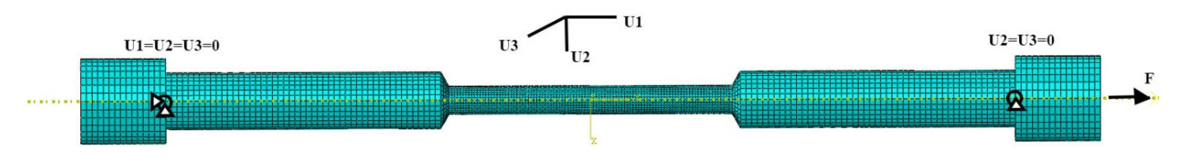
4.2. Numerical Simulation of Full-Scale Tensile Specimens

To simulate the ductile failure of the dog-bone-shaped tensile specimens, a three-dimensional model was constructed, replicating in detail the geometrical properties of the manufactured tensile specimens. After some initial mesh sensitivity analysis (Appendix C), the maximum size of C3D8R elements was chosen as equal to 3 mm × 2 mm × 2 mm (coarse mesh), and the minimum size at the working length was set as 1 mm × 1 mm × 1 mm (fine mesh), which resulted in a total of 25,344 elements (Figure 16). For the material modeling, parameters stated in Section 3 were used, and boundary conditions were utilized in accordance with the experimental setup. Similarly to the experimental procedure, quasi-static 0.001 s⁻¹ and 0.5 s⁻¹ strain rate uniaxial tensile simulations were performed, and the results can be seen in Figure 17. Similarly to the experimental process, in the case of numerical simulations, load and displacement were monitored throughout the uniaxial tensile test. Afterwards, the obtained load–displacement data were transformed into engineering stress–strain curves and, subsequently, to true stress–strain curves. Overall, good accuracy is observed between experimental and numerical results for both cases. In particular, for the quasi-static strain rate case, apart from some initial discrepancy in the post-yielding stress capacity (numerical results overestimate the experimental case by 2.6%) the stress–strain curve follows closely the experimental results, and a 2.4% difference in ultimate stress is observed. Furthermore, although the fracture strain between the numerical analysis and experimental results is similar, the numerical simulation retains a higher stress state for larger strain values decreasing sharply, leading to element failure. For the case of the 0.5 s⁻¹ strain rate, after yielding, the numerical model underestimates the experimental results by 2.7%, but after that, the numerical stress–strain curve follows closely the experimental one. Finally, a 3.6% difference is observed for the failure strain between numerical and experimental results. The above statements can be seen summarized in

Table 5. Comparison between experimental and numerical post-yield and ultimate stress states as well as fracture strains for 0.001 s⁻¹ and 0.5 s⁻¹ strain rates.

	Post-Yielding Stress (MPa)	Ultimate Stress (MPa)	Fracture Strain
Avg. Experimental 0.001 s−1 strain rate	997	1231	0.111
Numerical 0.001 s−1 strain rate	971	1261	0.101
0.001 s−1 strain rate error (%)	2.67	−2.4	0.1
Avg. Experimental 0.5 s−1 strain rate	1069	1272	0.087
Numerical 0.5 s−1 strain rate	1041	1271	0.084
0.5 s−1 strain rate error (%)	2.69	0.01	3.57

.

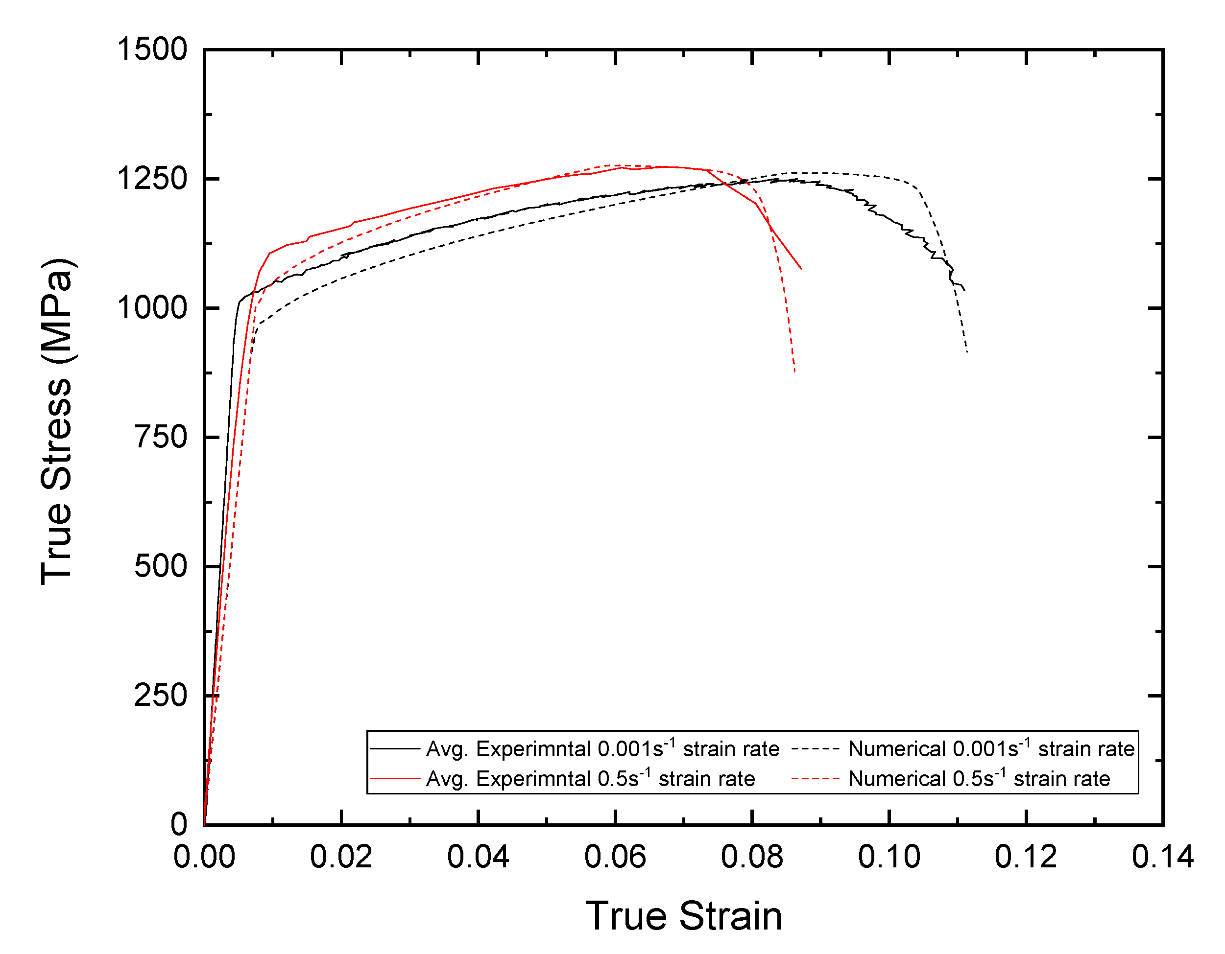
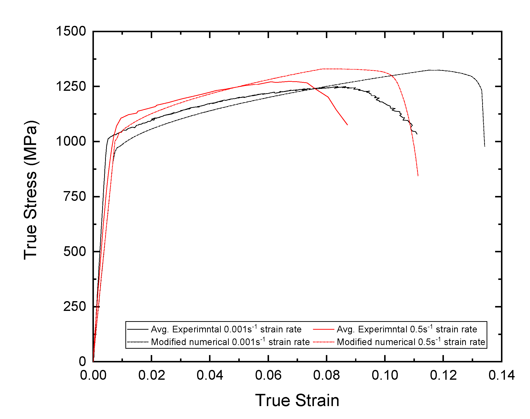
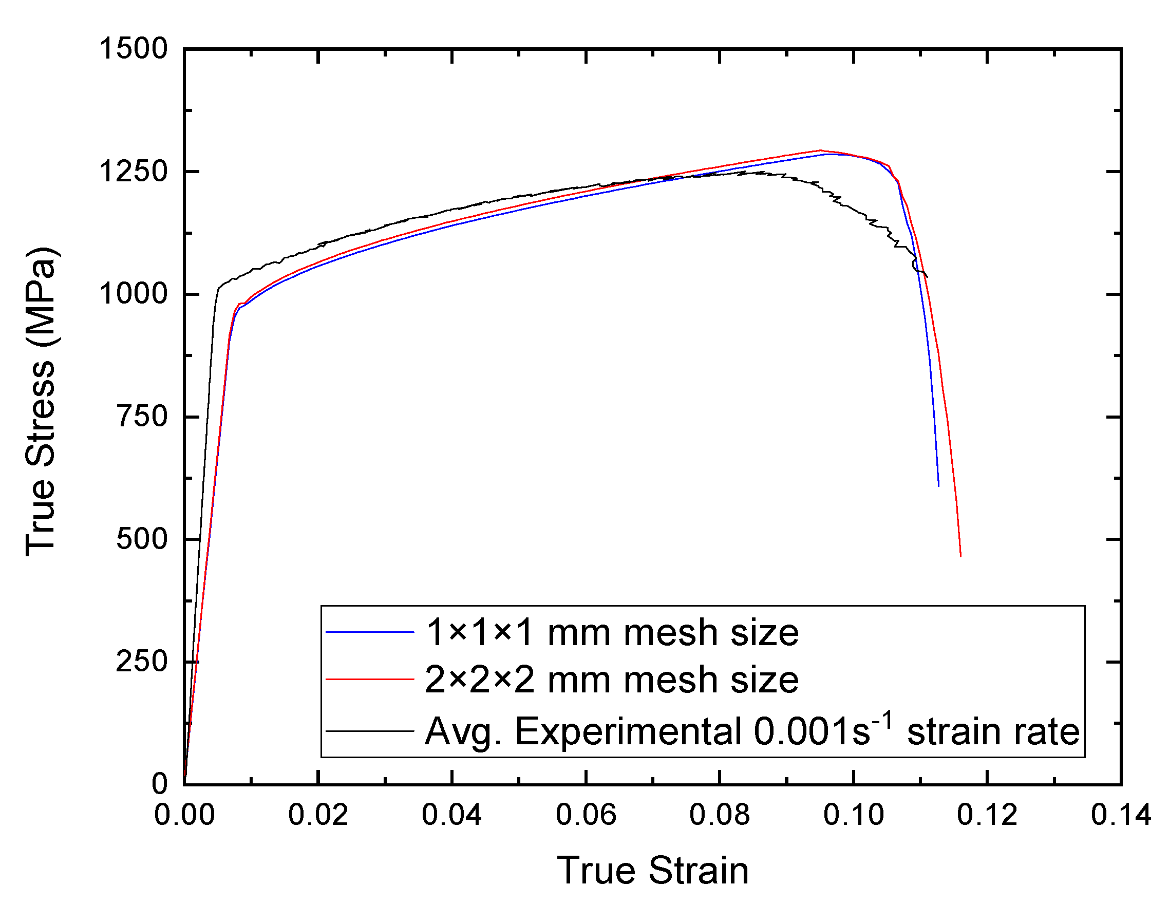
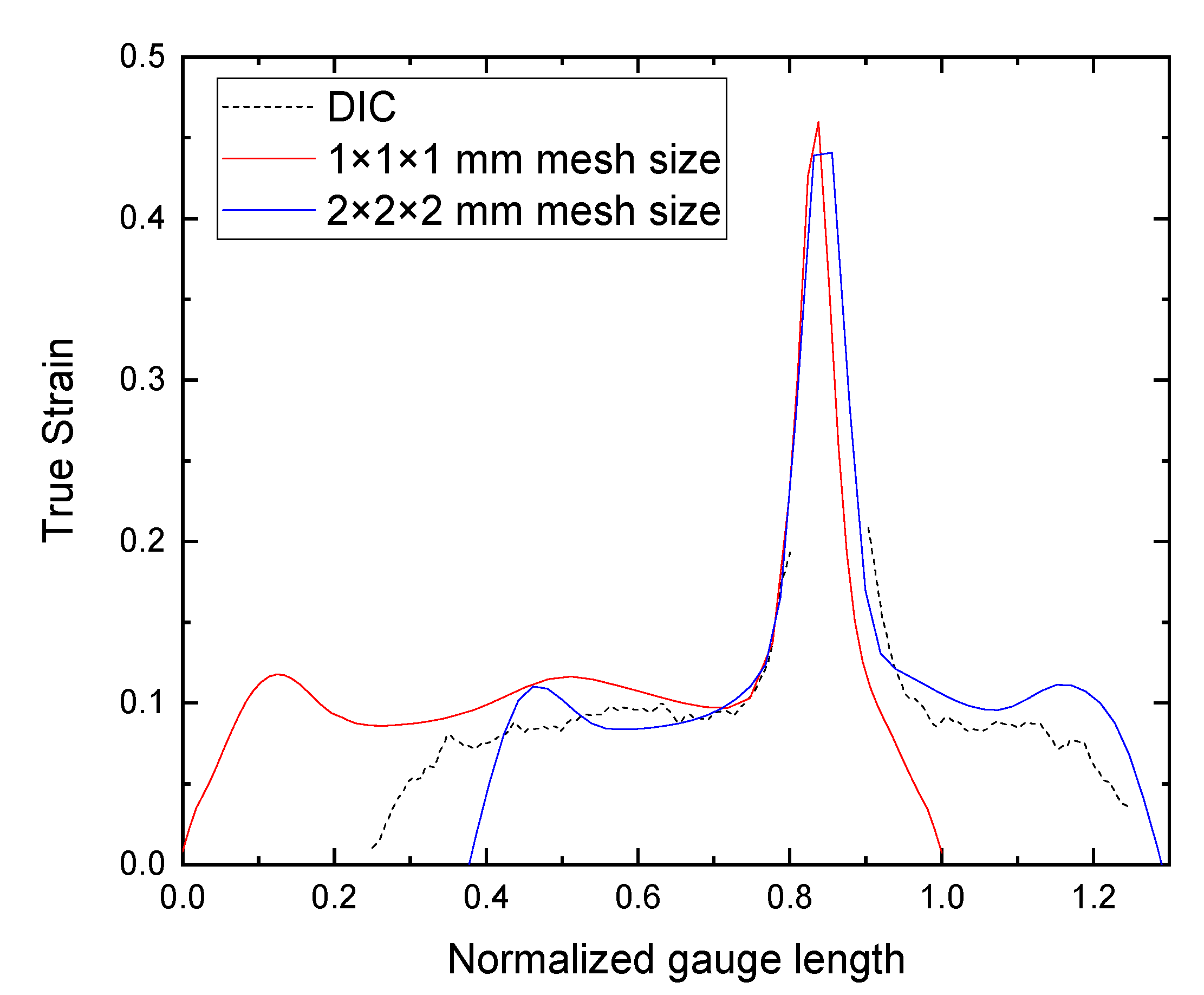
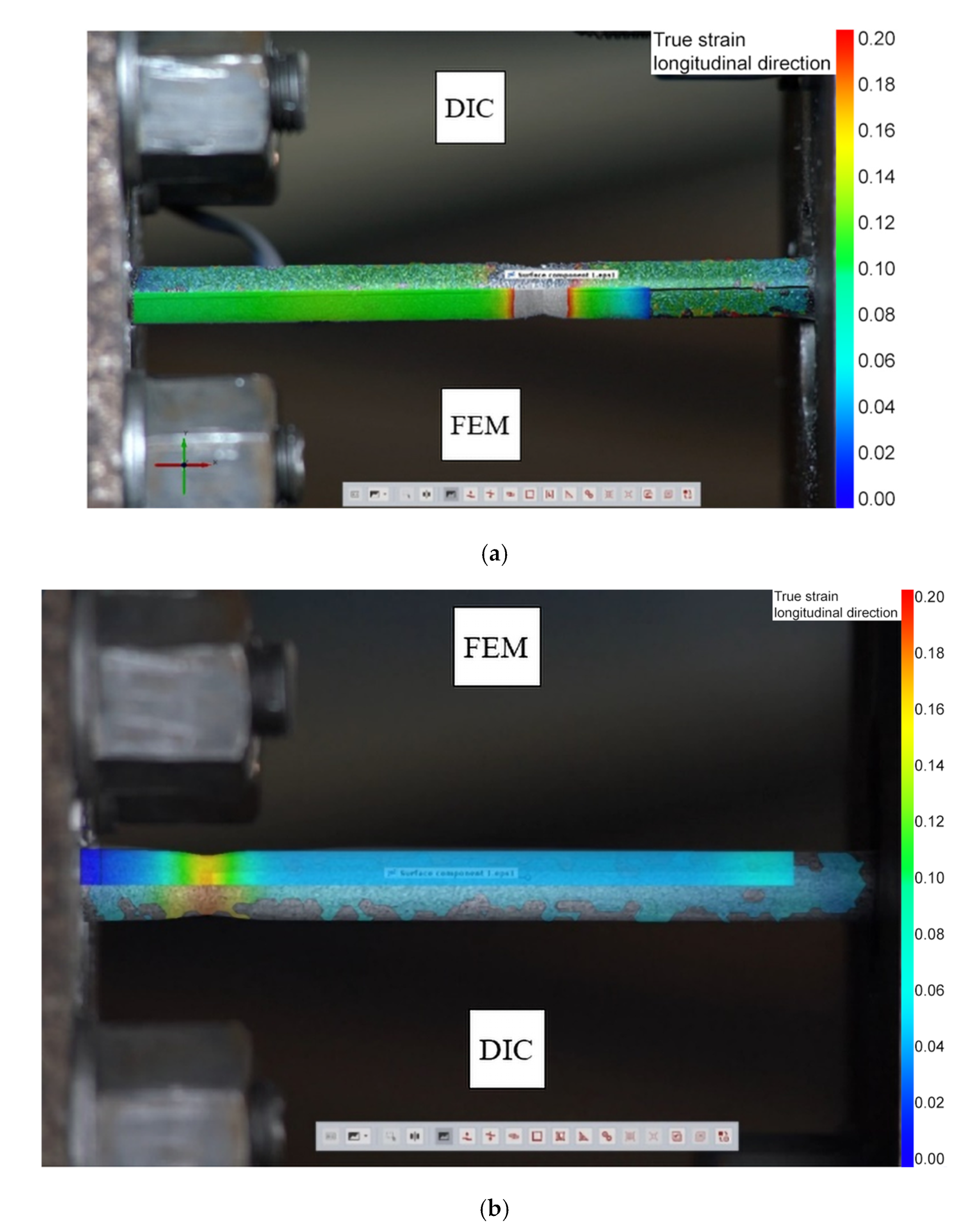
5. Numerical Model Verifications for Smooth Specimens

To further validate the accuracy of the JC flow stress model as well as the JC damage parameters that were calculated in the previous sections, DIC analysis was attempted for specimens subjected to uniaxial tension under different strain rates. To perform the DIC analysis, commercially available software was used called “GOM Correlate”. It is a DIC evaluation software program that is extensively used for material research and compound testing purposes. GOM Correlate follows a parametric approach that guarantees reliability for measuring required strains through a parametric approach. While using GOM Correlate, users have to define initial parameters regarding strain surface components for the area of interest, and the software creates facets which are square shaped across the whole range of supplied image data. Based on a high-contrast stochastic pattern that the user has to apply on the area of interest where strain is required to be measured, the software identifies these facets based on the quality of the aforementioned stochastic pattern. An additional parameter that requires adjustment from the user is the distance between adjacent facets on a center-to-center basis. This setting directly influences and it is correlated to the point density within the area of interest, and by decreased said distance, higher spatial resolution can be obtained by decreasing the distance of adjacent facets [28,29,30].

In this work, a full-frame CMOS camera was used to capture 1920 × 1080 pixel-sized image series and videos to be used for the DIC analysis. For DIC, the captured stochastic pattern (Figure 18) was processed using a facet size of 14 and a distance of 9 to evaluate the corresponding strain fields. To compare the experimental results with the numerical modeling, strain was recorded along the axis of the cylindrical specimens and was compared with the resulting strain in central nodes of the FE model. Due to camera limitations regarding video framerate capturing capabilities, as well as applied pattern-related shortcomings, although DIC analysis was attempted for all experimental cases, it was only successful for quasi-static and 0.5 s⁻¹ experimental cases. Namely, for higher strain-rates, to capture a significant amount of image series, 120 fps video recording was attempted, but only a resolution up to 1280 × 720 pixels was available. The lowered resolution coupled with brittleness of the coloring used to create the stochastic speckle pattern severely limited the amount of usable data for the DIC analysis. The resulting strain profile can be seen in Figure 19 for (a) the quasi-static tensile case and for (b) the dynamic case with a strain rate of 0.5 s⁻¹. In both Figure 19a,b, the horizontal axis data for finite element modeling (FEM) case have been shifted by an amount suitable to each case in order to align the portion of the gauge length in which necking and, correspondingly, fracture occurred. To aid with the visualization of the data, true strain and normalized gauge length data points are being used. For the quasi-static case, due to stochastic pattern degradation, strain data were captured up to approximately 0.2 strain.

When comparing the FEM analysis results with DIC for 0.001 s⁻¹ strain rate, around the area where necking occurs, high strain region is concentrated for 22.6% of the normalized length as opposed to the DIC, which is 26.5%, resulting in the tensile specimen forming a longer necking region by 3.9%. For the case of 0.5 s⁻¹ strain rate, even better accuracy is observed with the FEM results underestimating the length where necking occurs by 1.6%. Overall, in both cases, good accuracy is observed between the DIC and FEM results, further reinforcing the suitability of the proposed JC model and damage parameters for SBPR 930/1080 Type B No. 1 tendon high-strength material.

In Figure 20, the strain map results from DIC analysis and FE simulations are overlapped visualizing the results presented in Figure 19 for smooth specimens at the last captured frame before rupture. In each corresponding figure, FE simulation strain contours have been scaled to the value of DIC analysis, and the overlapping FEM image has been repositioned to align the necking region with the DIC image. As a result, in the case of 0.001 s⁻¹ strain rate, near the center of the necking region, the resulting strain values exceed the visualization boundary limits of 0.0–0.2 strain and, as a result, the region with a strain rate higher than these values are presented in grey color.

6. Conclusions and Recommendations

In this work, numerous tensile tests at room temperature and strain rates 0.001 s⁻¹–0.5 s⁻¹ were performed in order to calculate the Johnson–Cook model and damage parameters for SBPR 930/1080 Type B No. 1 tendon material aimed at fracture analysis of post-tensioned concrete members. Overall, the results obtained in this work, after the calculation of JC parameters, showed good agreement with the experimental data. To verify the agreement between numerical data and experimental tensile data, commercial FEM software was used. The experimental tensile tests were replicated in detail in order to verify the performance of the damage model using both experimental observations, experimental stress–strain data, as well as DIC analysis. The JC model is found to be able to closely predict experimental data with less effort in comparison to other analytical models, but on the other hand, to properly calibrate the related parameters, extensive numerical data are required from several experimental cases. It was found that besides small prediction differences between the FE simulation and experimental results, good accuracy was achieved in predicting the effects of strain concentration and geometrical deformation (necking). Based on these research outcomes, the followed procedure can be applied to closely predict the performance of tested material for fracture analysis of post-tensioned concrete members.

As for recommendations, in this work, all testing was performed at room temperature, and thus, we were not able to identify damage-related parameters with regard to material softening under elevated temperatures; therefore, further testing could be performed to identify these parameters, and dynamic testing could be performed under even higher strain rates, in order to gain a broader picture of strain-related hardening effects. Furthermore, by utilizing the JC model and damage parameters presented in this work, researchers can simulate and estimate the remaining strength of a damaged or corroded PC tendon. By measuring or estimating the remaining cross-section of a tendon, it is possible to accurately estimate stress-concentration states surrounding the damaged or corroded area and construct relevant fragility curves based on the anticipated loading conditions.

References

1. Pape, T.M.; Melcher, R.E. Performance of 45-year-old corroded prestressed concrete beams. Proc. Inst. Civ. Eng. Struct. Build. 2013, 166, 547–559. [Google Scholar] [CrossRef] [Green Version]
2. Abdelatif, A.O.; Owen, J.S.; Hussein, M.F.M. Re-anchorage of a ruptured tendon in bonded post-tensioned concrete beams: Model validation. Key Eng. Mater. 2013, 569–570, 302–309. [Google Scholar] [CrossRef] [Green Version]
3. Jeon, C.H.; Shim, C.S. Flexural behavior of post-tensioned concrete beams with multiple internal corroded strands. Appl. Sci. 2020, 10, 7994. [Google Scholar] [CrossRef]
4. Trejo, D.; Hueste, M.B.D.; Gardoni, P. Effect of Voids in Grouted, Post-Tensioned Concrete Bridge Construction: Volume 1-Electrochemical Testing and Reliability Assessment 5. Report Date 13. Type of Report and Period Covered Unclassified. 2009. Available online: https://static.tti.tamu.edu/tti.tamu.edu/documents/0-4588-1-Vol1.pdf (accessed on 19 January 2022).
5. Coronelli, D.; Castel, A.; Vu, N.A.; François, R. Corroded post-tensioned beams with bonded tendons and wire failure. Eng. Struct. 2009, 31, 1687–1697. [Google Scholar] [CrossRef]
6. Tamakoshi, T.; Hiraga, K.; Kimura, Y. A Case Study of Corrosion Damage of PC Steel-Investigation of Grout Unfilling and Steel Corrosion of Myoko Bridge. Civ. Eng. J. 2012, 54, 50–51. [Google Scholar]
7. Jeon, C.H.; Nguyen, C.D.; Shim, C.S. Assessment of mechanical properties of corroded prestressing strands. Appl. Sci. 2020, 10, 4055. [Google Scholar] [CrossRef]
8. Wuertemberger, L.; Palazotto, A.N. Evaluation of Flow and Failure Properties of Treated 4130 Steel. J. Dyn. Behav. Mater. 2016, 2, 207–222. [Google Scholar] [CrossRef] [Green Version]
9. Khataei, M.; Poursina, M.; Kadkhodaei, M. A study on fracture locus of St12 steel and implementation ductile damage criteria. AIP Conf. Proc. 2010, 1252, 1303–1308. [Google Scholar] [CrossRef]
10. Murugesan, M.; Jung, D.W. Johnson cook material and failure model parameters estimation of AISI-1045 medium carbon steel for metal forming applications. Materials 2019, 12, 609. [Google Scholar] [CrossRef] [Green Version]
11. Banerjee, A.; Dhar, S.; Acharyya, S.; Datta, D.; Nayak, N. Determination of Johnson cook material and failure model constants and numerical modelling of Charpy impact test of armour steel. Mater. Sci. Eng. A 2015, 640, 200–209. [Google Scholar] [CrossRef]
12. Johnson, G.R.; Cook, W.H. Fracture characteristics of three metals subjected to various strains, strain rates, temperatures and pressures. Eng. Fract. Mech. 1985, 21, 31–48. [Google Scholar] [CrossRef]
13. Xu, K.; Wong, C.; Yan, B.; Zhu, H. A High Strain Rate Constitutive Model for High Strength Steels; SAE Technical Paper; SAE International: Warrendale, PN, USA, 2003; ISSN 0148-7191. [Google Scholar] [CrossRef]
14. Vedantam, K.; Bajaj, D.; Brar, N.S.; Hill, S. Johnson-Cook strength models for mild and DP 590 steels. AIP Conf. Proc. 2006, 845, 775–778. [Google Scholar] [CrossRef]
15. JIS G 3109 2010; Steel Bars for Prestressed Concrete. Japan Industrial Standard (JIS): Tokyo, Japan, 2010.
16. Samantaray, D.; Mandal, S.; Bhaduri, A.K. A comparative study on Johnson Cook, modified Zerilli–Armstrong and Arrhenius-type constitutive models to predict elevated temperature flow behaviour in modified 9Cr–1Mo steel. Comput. Mater. Sci. 2009, 47, 568–576. [Google Scholar] [CrossRef]
17. Akbari, Z.; Mirzadeh, H.; Cabrera, J.M. A simple constitutive model for predicting flow stress of medium carbon microalloyed steel during hot deformation. Mater. Des. 2015, 77, 126–131. [Google Scholar] [CrossRef] [Green Version]
18. Maheshwari, A.K. Prediction of flow stress for hot deformation processing. Comput. Mater. Sci. 2013, 69, 350–358. [Google Scholar] [CrossRef]
19. He, A.; Xie, G.; Zhang, H.; Wang, X. A comparative study on Johnson–Cook, modified Johnson–Cook and Arrhenius-type constitutive models to predict the high temperature flow stress in 20CrMo alloy steel. Mater. Des. 2013, 52, 677–685. [Google Scholar] [CrossRef]
20. Wang, X.; Shi, J. Validation of Johnson-Cook plasticity and damage model using impact experiment. Int. J. Impact Eng. 2013, 60, 67–75. [Google Scholar] [CrossRef]
21. Murugesan, M.; Lee, S.; Kim, D.; Kang, Y.H.; Kim, N. A Comparative Study of Ductile Damage Models Approaches for Joint Strength Prediction in Hot Shear Joining Process. Procedia Eng. 2017, 207, 1689–1694. [Google Scholar] [CrossRef]
22. Bai, Y.; Wierzbicki, T. A new model of metal plasticity and fracture with pressure and Lode dependence. Int. J. Plast. 2008, 24, 1071–1096. [Google Scholar] [CrossRef]
23. Bao, Y. Dependence of ductile crack formation in tensile tests on stress triaxiality, stress and strain ratios. Eng. Fract. Mech. 2005, 72, 505–522. [Google Scholar] [CrossRef]
24. Bridgman, P. Studies in Large Plastic Flow and Fracture with Special Emphasis on the Effects of Hydrostatic Pressure, 1st ed.; McGraw-Hill: New York, NY, USA, 1952. [Google Scholar]
25. Bao, Y.; Wierzbicki, T. On fracture locus in the equivalent strain and stress triaxiality space. Int. J. Mech. Sci. 2004, 46, 81–98. [Google Scholar] [CrossRef]
26. Dassault Systemes Simulia. Abaqus; Dassault Systemes Simulia: Providence, RI, USA, 2021. [Google Scholar]
27. Dassault Systemes Simulia. Abaqus Analysis User’s Manual; Dassault Systemes Simulia: Providence, RI, USA, 2021. [Google Scholar]
28. GOM GmbH. GOM Correlate. GOM-Precise Industrial 3D Metrology, Braunschweig, Germany. Available online: https://www.gom.com/index.html (accessed on 22 May 2021).
29. GOM GmbH. Inspection—3D Testing. In GOM Correlate Professional V8 SR1 Manual Basic; GOM mbH: Braunschweig, Germany, 2015. [Google Scholar]
30. GOM GmbH. Digital Image Correlation and Strain Computation Basics. In GOM Testing-Technical Documentataion; GOM mbH: Braunschweig, Germany, 2015. [Google Scholar]
31. Hillerborg, A.; Modéer, M.; Petersson, P.E. Analysis of crack formation and crack growth in concrete by means of fracture mechanics and finite elements. Cem. Concr. Res. 1976, 6, 773–781. [Google Scholar] [CrossRef]
Figure 1. Deteriorated strands in bridges due to corrosion: (a) complete failure (reproduced with permission from ref. [6]; 2012; T. Tamakoshi et al.) (b) severe deterioration (figure adapted from ref. [7]; 2020; C. H. Jeon et al.).
Applsci 12 07774 g001
Figure 2. Geometrical details of specimens for tensile tests at (a) smooth-type quasi-static and dynamic strain rates, (b) notched R0.4 type, (c) notched R20 type, (d) notched R50 type and (e) detailed representation of notched region; (f) typical manufactured specimen.
Applsci 12 07774 g002
Figure 3. Experimental setup.
Applsci 12 07774 g003
Figure 4. Servo-hydraulic MTS 244.11 technical specifications.
Applsci 12 07774 g004
Figure 5. Detailed specimen fixture mechanism.
Applsci 12 07774 g005
Figure 6. Engineering stress–strain (a) and true stress–strain (b) curves for uniaxial tensile tests under different strain rates.
Applsci 12 07774 g006
Figure 7. Engineering stress–strain (a) and true stress strain (b) curves for uniaxial tests with different notch sizes.
Applsci 12 07774 g007
Figure 8. ln(σ − A) and lnε relationship under reference conditions.
Applsci 12 07774 g008
Figure 9. Relationship between σ ( A + B ε ) n and l n ε ˙ * for four different strain rates (0.001 s−1, 0.5 s−1, 1 s−1, 2 s−1).
Applsci 12 07774 g009
Figure 10. Comparison of true stress–strain curve between experimental data and JC analytical prediction.
Applsci 12 07774 g010
Figure 11. Fracture strain and stress triaxiality relationship from uniaxial tensile test data.
Applsci 12 07774 g011
Figure 12. Relationship between ε f D 1 + D 2 e D 3 η * and ln ε ˙ * .
Applsci 12 07774 g012
Figure 13. (a) Singular element’s boundary conditions used in FE simulation; (b) smooth piecewise application of velocity amplitude.
Applsci 12 07774 g013
Figure 14. Comparison between experimental (Exp, continuous lines) and FE simulation (Sim, dotted lines) results for 0.001 s−1–2 s−1 strain rates.
Applsci 12 07774 g014
Figure 15. (a) Stress–strain behavior of a characteristic material undergoing progressive damage (Abaqus Analysis User’s Manual 2021) and (b) correlation between damage parameter and equivalent plastic strain used to model softening behavior of the material in this work under reference conditions.
Applsci 12 07774 g015
Figure 16. Mesh and boundary conditions used for numerical modeling of smooth tensile specimens.
Applsci 12 07774 g016
Figure 17. True stress–strain plot comparison for 0.001 s−1 and 0.5 s−1 strain rates for average experimental and numerical simulation using modified (Table 4) JC damage parameters.
Applsci 12 07774 g017
Figure 18. Stochastic speckle pattern used for DIC analysis during (a) beginning of the tensile test and (b) one frame before rupture.
Applsci 12 07774 g018
Figure 19. Comparison plots for true strain and normalized gauge length of tensile specimens between data points obtained from DIC analysis and FE simulation for (a) 0.001 s−1 and (b) 0.5 s−1 strain rates.
Applsci 12 07774 g019
Figure 20. Visual comparison between DIC analysis and FE simulation strain map results for smooth specimens at the last captured frame before rupture for (a) 0.001 s−1 and (b) 0.5 s−1 strain rates.
Applsci 12 07774 g020