The Analysis of WJ Distribution as an Extended Gaussian Function: Case Study

Abstract

The double exponential WJ distribution has been shown to competently describe extreme events and critical phenomena, while the Gaussian function has celebrated rich applications in many other fields. Here we present the analysis that the WJ distribution may be properly treated as an extended Gaussian function. Based on the Taylor expansion, we propose three methods to formulate the WJ distribution in the form of Gaussian functions, with Method I and Method III being accurate and self-consistent, and elaborate the relationship among the parameters of the functions. Moreover, we derive the parameter scaling formula of the WJ distribution to express a general Gaussian function, with the work illustrated by a classical case of extreme events and critical phenomena and application to topical medical image processing to prove the effectiveness of the WJ distribution rather than the Gaussian function. Our results sturdily advocate that the WJ distribution can elegantly represent a Gaussian function of arbitrary parameters, whereas the latter usually is not able to satisfactorily describe the former except for specific parameter sets. Thus, it is conclusive that the WJ distribution offers applicability in extreme events and critical phenomena as well as processes describable by the Gaussian function, namely, implying plausibly a unifying approach to the pertinent data processing of those quite distinct areas and establishing a link between relevant extreme value theories and Gaussian processes.

1. Introduction

1.1. Backgrounds

With profound theoretical interests and numerous practical applications, probability distribution functions are powerful apparatuses to describe stochastic random processes and statistical results, classically exemplified by the Gaussian function (normal distribution), exponential decay functions, and the Poisson function, among others [1,2,3,4,5,6]. Particularly prominent, the Gaussian function distinguishes itself in many ways, and the statistics of many sampling spaces show a tendency to become a normal distribution as the sampling sizes increase. As a matter of fact, Gaussian distributions take place broadly in both natural and social sciences and occupy a key position in mathematics, physics, and engineering. Mathematically, the Gaussian function has its unique role in defining the Hermite polynomials, as typical kernels of Green’s functions and in applying the Bayesian inference. In probability statistics, both t-distribution and binomial distribution eventually trend to the Gaussian distribution, from which t-distribution and F-distribution are derivable. Multivariate and multidimensional methods involving generalized Gaussian functions have been developed for advanced applications [7]. In the field of communications, the Gaussian function is incurred to quantify the statistical behaviors of channel noises, bit error rates, image processing, and multimedia signal enhancement [8], as well as the response peak of chromatographic detection [9]. In physics, Gaussian functions are introduced to work out thermodynamic and diffusion equations [10,11], define Gaussian light beams [12] and have superior niches as the wave function describing the ground state of a quantum harmonic oscillator, as molecular orbitals through their proper linear combinations and being related to the vacuum state in quantum field theory. Medical phenomena such as mass population heights, red blood cell numbers, and hemoglobin amounts are adequate to be characterized or approximated by Gaussian distributions, with multidimensional-multivariate generalizations in perspective. To a certain extent, researches in educational statistics confirm that students’ academic performance and practical ability seem to follow Gaussian propensities. In reality, the Gaussian distribution is a milestone in the development history of statistical theory, with the probability density function as

$$f\left(x,{\mu }_{GS},\sigma \right)=\frac{1}{\sqrt{2\pi }\sigma }{e}^{-\frac{{(x-{\mu }_{GS})}^2}{2{\sigma }^2}}$$

(1a)

where $\sigma$ and ${\mu }_{GS}$ are the respective standard deviation and expectation of a random process, defined over the domain of (−∞, +∞). The commonly used form of Equation (1a) is known as the standard normal distribution when ${\mu }_{GS}=0$ and $\sigma =1$, simply stated as

$$f\left(x,{\mu }_{GS}=0,\sigma =1\right)=\frac{1}{\sqrt{2\pi }}{e}^{-\frac{x^2}{2}}$$

(1b)

It appears relevant to emphasize that the parameters $\sigma$ and ${\mu }_{GS}$ are independent of each other, i.e., the former affects solely the shape of the curve while the latter exclusively determines the location of its center (which is markedly different from the WJ distribution as discoursed below [13]. As a note for the WJ distribution, we have wanted a short term to represent the distribution for the simplicity of discussion and come up with the abbreviation WJ which could mean wild, wide, or weird, even wonder jittering to reflect unusual occurrences such as extreme events and critical phenomena).

The WJ distribution function shows a universal mechanism to account for extreme events and critical phenomena [13], to which the Gaussian function is hard to be applied and frequently happens in nature and society, from extraordinary occurrences to critical properties, immensely diverse in types and dissimilar in properties [13,14,15,16]. In coping with such extreme events, actually, a series of classical distributions have been proposed comprising the Gumbel distribution, the Bramwell–Holdsworth–Pinton distribution, and the generalized Gumbel distribution [14,15,16], all of which may find a unification in the WJ distribution function [13]. Moreover, the WJ distribution function offers pertinent elucidation for the Kohlrausch-Williams-Watts (KWW) relaxation [17], the glass transition of glass-forming materials [17], and information theory [18]. Furthermore, closely related studies are electroencephalographic recordings of rodents with induced ischemic stroke [19], the transient current of organic field-effect transistors [20], and quantifying the effect of the presence of linear chains on the orientation dynamics of the rings [21].

1.2. Important Application of WJ Distribution to KWW Relaxation

As an important example from the direct application of the WJ distribution [17], it is constructive to emphasize that the proposal is constructed on the basis of the WJ distribution to interpret the underlying mechanism of the famous KWW relaxation function [13,22,23]. Showing the ubiquitous irreversibility characteristics on the atomic, molecular, or electronic scale and the dynamic nature of irreversible processes, the KWW relaxation function or the stretched exponential relaxation function is a phenomenal observation in complex systems from the intricate behavior of liquids and glasses, the folding of proteins to the structure and dynamics of atomic and molecular clusters and well delineating the phenomena of important time-dependent dynamic processes [13,22,23]. The research has a long history of continuous interest, research inputs, and technological importance, in condensed matter physics in particular, as manifested by the fact that our research outcomes [17] have prompted wide attention from diverse fields [23,24,25,26,27,28,29,30,31,32,33,34].

1.3. More Non-Gaussian Distributions

It should be adequate to point out that the list of non-Gaussian or skewed Gaussian distributions, including the Gaussian distribution and working well in practice, is truly long [1,35], encompassing the well-established Weibull distributions [23,35,36], Levy distributions [27,35], skew-normal and related families [37,38,39,40], Beta distributions [35], lognormal distributions [35], multivariate normal distributions [7,35], multidimensional normal distributions [7,35], gamma distributions [35], hypergeometric distributions [35] and Cauchy distributions [35] in addition to the above-mentioned models concerning extreme events and critical phenomena [13,14,15,16].

1.4. Some Initial Considerations of the WJ Distribution

The WJ distribution is a double exponential function [13]

$$f\left(x,\alpha ,\beta ,\nu \right)=\frac{\beta }{\Gamma \left(\alpha /\beta \right)}{e}^{-\alpha \left(x-\nu \right)-e^{-\beta \left(x-\nu \right)}}$$

(2)

or equivalently

$$f\left(x,\alpha ,\beta ,{\mu }_{WJ}\right)=\frac{\beta }{\Gamma \left(\alpha /\beta \right)}{e}^{-\alpha \left[x-{\mu }_{WJ}-\frac{1}{\beta }\Psi \left(\frac{\alpha }{\beta }\right)\right]-e^{-\beta \left[x-{\mu }_{WJ}-\frac{1}{\beta }\Psi \left(\frac{\alpha }{\beta }\right)\right]}}$$

(3)

with $\nu ={\mu }_{WJ}+\Psi \left(\alpha /\beta \right)/\beta$, defined over the domain of (−∞, +∞). In terms of Equations (2) or (3), the WJ function has three parameters $\alpha$, $\beta$ and ${\mu }_{WJ}$: The parameter ${\mu }_{WJ}$ shifts the location of the curve but does not affect the shape of the distribution (we may set it to 0 just for the sake of discussion). The parameters $\alpha$and $\beta$ taking positive values jointly determine the shape of the curve and make a contribution of $\Psi \left(\alpha /\beta \right)/\beta$ to the horizontal position of the curve.

In contrast to the symmetric shape of the Gaussian curve about the line $x={\mu }_{GS}$, the characteristics of the WJ distribution are more complex and assorted with changes in the parameters α and β (as deliberated later in the text, such curves can behave similarly to the Gaussian for specific sets of α and β). A more direct intuition of the behavior of the WJ distribution is unquestionably beneficial from 2D plotting by fixing the ratio of $\alpha$ to $\beta$ in the scaled form of $f_{WJ}\left(x,\alpha ,\beta ,{\mu }_{WJ}\right)\Gamma \left(\alpha /\beta \right)/\beta$ vs. ($x-\nu$), as shown in Figure 1. Figure 1a exhibits the cases of $\alpha /\beta =1$ and $\alpha \in$ (0.5, 1, 2, 3, 4). The various kinds of curves demonstrate an asymmetrical bell-like shape and tighten the distribution as the $\alpha$ value increases (and the $\beta$ value increases simultaneously), with the peaks roughly located at the same position. Figure 1b sums up the results of setting $\alpha /\beta =2$ and $\beta \in$ (0.5, 1, 2, 3, 4), in which the curves are characterized by tightening the shapes and a right-shifting of the maxima with an increasing value of $\beta$. Comparing Figure 1a with Figure 1b, the curves look more symmetrical when $\alpha /\beta =2$. Purportedly, the WJ distribution with proper choices of $\alpha$ and $\beta$ can be highly symmetrical like a Gaussian function, sharing some characteristics in common.

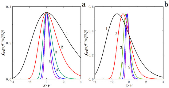
Figure 1. Effects of the parameters $\alpha$ and $\beta$ on the behavior of the WJ distribution. (a) Curves 1~5 in order correspond to $\alpha \in$(0.5, 1, 2, 3, 4) for $\alpha /\beta =1$; (b) Curves 1~5 in order correspond to $\beta \in$(0.5, 1, 2, 3, 4) for $\alpha /\beta =2$.

1.5. Content of This Work

To the best of our knowledge, there is no report on linking extreme value theories and the Gaussian function as representable by a possible relation between the WJ distribution and the Gaussian function yet. In this work, we are going to establish such bridging and give a primary objective to establish that the Gaussian function may presumably be treated as a subclass of the WJ distribution. In the next sections, we shall explore the transformation between the WJ distribution and the Gaussian function by the technique of the Taylor expansion. The lines of deliberation run along the Taylor expansion at three distinct points, i.e., around x = 0 (Method I), x = ν (Method II) and x = x_m (Method III), properly elaborated with numerical solutions. For Method I, in particular, we show in detail that for properly selected sets of the parameters, such an approximation of the WJ distribution to the Gaussian function is indeed quite good. Thereon, we develop the parameter scaling relations how to definitely express the general Gaussian function by the WJ distribution. The work is highlighted by a classical case of extreme events and critical phenomena and applications to current medical imaging analyses to attest to the usefulness of the WJ distribution in preference to the Gaussian function and endorse a scheme integrating both Gaussian processes and non-Gaussian ones such as extreme events and critical phenomena.

1.6. Contribution of This Work

Concisely, we have proven for the first time that the two parametric Gaussian functions may be treated as a special subclass of a tri-parametric WJ distribution for specific parameter sets, or alternatively, the WJ distribution can be appropriately considered as an extended Gaussian function. Building up a connection between extreme value theories and Gaussian processes, moreover, the study shows that the WJ distribution has fundamental interests and advanced applications in critical phenomena, extreme occurrences, and processes such as topical medical image processing that can be described by the Gaussian function. Our proposal of transforming the WJ distribution to the Gaussian function through proper Taylor expansion offers a plausible unifying, broad approach to promoting comprehensive mechanistic understandings on the basis of integrated data processing in those very different fields. Thus, our work has topicality and assumes theoretical impact and applicational usefulness.

2. Methods

2.1. Theoretical Considerations

The Taylor expansion method was applied to convert the WJ distribution to the form of a Gaussian function. The expansion was performed around three representative positions, i.e., around x = 0 (Method I), x = ν (Method II) or x = x_m (Method III). The expansion outcomes were appropriately elucidated with numerical solutions. The fitting methods adopted were nonlinear regressions, and the overall goodness-of-fit criterion was the correlation coefficient R² (COD, Coefficient of Determination), supported by the analysis of the residual errors for individual points.

2.2. Methodological Considerations

The software packages Matlab 2017a (downloaded from the site http://xxb.njupt.edu.cn/MATLAB/list.htm, accessed on 6 July 2022) and Origin 2021 (downloaded from the site https://www.originlab.com/, accessed on 6 July 2022) were employed in our computation, and commercial laptop computers were used to execute the programs. The runtime typically took less than 10 s.

3. Results and Discussion

In the study, we have found that the WJ distribution may give a proper description of the properties of the Gaussian function, which is attributable to the fact that the WJ distribution in a double exponential form is capable of being converted to the expression of a Gaussian function by a proper Taylor expansion of it with a truncation of the resulted series. Below we carry out detailed analyses of the results from the Taylor expansion of the WJ distribution in three different ways (methods).

3.1. Method I

3.1.1. Development of the Method

We first expand the term of $e^{-\beta x}$ in the exponential part $e^{-\beta \left(x-\nu \right)}$ in Equation (2) on the basis of the Taylor formula around the point $x=0$, explicitly,

$$e^{-\beta x}={\displaystyle {{\displaystyle \sum }}_{n=0}^{\infty }}\frac{{(-1)}^n{\beta }^n{x}^n}{n!},$$

then carry out the substitution, giving

$$f\left(x,\alpha ,\beta ,\nu \right)=\frac{\beta }{\Gamma \left(\alpha /\beta \right)}{e}^{-\alpha \left(x-\nu \right)-e^{\beta \nu }{\displaystyle \sum }_{n=0}^{\infty }\frac{{(-1)}^n{\beta }^n{x}^n}{n!}}$$

(4)

Considering the truncation of the terms after $x^2$ when the value of $\beta x$ is small enough, we take the first three terms in the sum

$${\displaystyle \sum }_{n=0}^{\infty }\frac{{(-1)}^n{\beta }^n{x}^n}{n!}=1-\beta x+\frac{{\beta }^2{x}^2}{2}+O\left({\beta }^3{x}^3\right)$$

and acquire the approximate expression for the WJ function in the form of

$$f_{\mathsf{{\rm I}}}\left(x,\alpha ,\beta ,\nu \right)=\frac{\beta }{\Gamma \left(\alpha /\beta \right)}{e}^{-\frac{e^{\beta \nu }{\beta }^2{x}^2}{2}-\left(\alpha -\beta e^{\beta \nu }\right)x+\alpha \nu -e^{\beta \nu }}$$

(5)

The exponential part of Equation (5) is subsequently rearranged to the square form about x (i.e., the exponential term of a Gaussian function) as

$$f_{\mathsf{{\rm I}}}\left(x,\alpha ,\beta ,\nu \right)=\frac{\beta e^{\frac{{(\beta e^{\beta \nu }-\alpha )}^2}{2e^{\beta \nu }{\beta }^2}+\alpha \nu -e^{\beta \nu }}}{\Gamma \left(\alpha /\beta \right)}{e}^{-\frac{{\beta }^2{e}^{\beta \nu }{(x-\frac{\beta e^{\beta \nu }-\alpha }{{\beta }^2{e}^{\beta \nu }})}^2}{2}}$$

(6)

As Equation (6) is the result of truncating the Taylor expansion to second order, however, the expression is not certainly normalized as a probability distribution. To guarantee the normalization and still a good approximation to a Gaussian function, we adopt the line of rationalization: Comparing the equation with the formulation of the Gaussian function in Equation (1a), we have two options for the estimation of $\sigma$, exponential based and prefactor based, that is,

$${\widehat{\sigma }}_{\mathsf{{\rm I}}1}=\sqrt{\frac{1}{{\beta }^2{e}^{\beta \nu }}}$$

(7)

and

$${\widehat{\sigma }}_{\mathsf{{\rm I}}2}=\frac{\Gamma \left(\alpha /\beta \right)}{\sqrt{2\pi }\beta e^{\frac{{\alpha }^2}{2e^{\beta \nu }{\beta }^2}-\frac{\alpha }{\beta }+\alpha \nu -\frac{e^{\beta \nu }}{2}}}$$

(8)

With regards to the expectation ${\mu }_{GS}$, we have its estimation of ${\widehat{\mu }}_{\mathsf{{\rm I}}}$,

$${\widehat{\mu }}_{\mathsf{{\rm I}}}=\frac{\beta e^{\beta \nu }-\alpha }{{\beta }^2{e}^{\beta \nu }}$$

(9)

Therefore, we have come to the two equations, (7) and (8), for estimating $\sigma$ on the basis of the parameters of the WJ distribution function. In combination with Equation (9), two normal distributions $\mathrm{N}\left({\widehat{\mu }}_{\mathsf{{\rm I}}},{\widehat{\sigma }}_{\mathsf{{\rm I}}1}\right)$ and $\mathrm{N}\left({\widehat{\mu }}_{\mathsf{{\rm I}}},{\widehat{\sigma }}_{\mathsf{{\rm I}}2}\right)$ are available to approximate the WJ distribution to be expressed as Gaussian functions, labeled respectively as CaseI1 and CaseI2 for the convenience of discussion. In explicit, the expressions representing the normal distributions are

$$f_{\mathsf{{\rm I}}1}\left(x,\alpha ,\beta ,\nu \right)=\frac{\beta e^{\beta \nu /2}}{\sqrt{2\pi }}{e}^{-\frac{{\beta }^2{e}^{\beta \nu }{(x-\frac{\beta e^{\beta \nu }-\alpha }{{\beta }^2{e}^{\beta \nu }})}^2}{2}}$$

(10)

for $\mathrm{N}\left({\widehat{\mu }}_{\mathsf{{\rm I}}},{\widehat{\sigma }}_{\mathsf{{\rm I}}1}\right)$ and

$$f_{\mathsf{{\rm I}}2}\left(x,\alpha ,\beta ,\nu \right)=\frac{\beta e^{\frac{{(\beta e^{\beta \nu }-\alpha )}^2}{2e^{\beta \nu }{\beta }^2}+\alpha \nu -e^{\beta \nu }}}{\Gamma \left(\alpha /\beta \right)}{e}^{-\pi {(\frac{\beta e^{\frac{{\alpha }^2}{2e^{\beta \nu }{\beta }^2}-\frac{\alpha }{\beta }+\alpha \nu -\frac{e^{\beta \nu }}{2}}}{\Gamma \left(\frac{\alpha }{\beta }\right)})}^2{(x-\frac{\beta e^{\beta \nu }-\alpha }{{\beta }^2{e}^{\beta \nu }})}^2}$$

(11)

for $\mathrm{N}\left({\widehat{\mu }}_{\mathsf{{\rm I}}},{\widehat{\sigma }}_{\mathsf{{\rm I}}2}\right)$.

3.1.2. Numerical Appraisal: As an Accurate, Self-Consistent Method

As the important special case of the general Gaussian function (1a), we shall first focus on the aspects of analysis based on the standard normal distribution $x~\mathrm{N}\left(0, 1\right)$, which can be recovered from the former by the transform of

$$x=\frac{y-u_{GS}}{\sigma } .$$

The relevant interval probability is evaluable by the expression

$$P(a<x<b)=\Phi \left(\frac{b-{\mu }_{GS}}{\sigma }\right)-\Phi \left(\frac{a-{\mu }_{GS}}{\sigma }\right)$$

($\Phi \left[\left(x-{\mu }_{GS}\right)/\sigma \right)]$ is the cumulative probability function of the normal distribution). Illuminating the relationship between the WJ function and the normal distribution, the assessing procedure proceeds in the following way: Appropriately select a set of discrete points from the standard normal distribution (1b) as an experimental dataset, then fit it with the WJ distribution (2) and thus obtain the corresponding parameters ${\alpha }_0=12.52$,${\beta }_0=0.07915$and ${\nu }_0=63.96$ ($R^2\approx 0.9997$). As shown in Figure 2a, in which the dots are the Gaussian values, and the curve is the fitting outcome of the WJ function, it is clear that both of them match optimally and are consistent with the almost unity of the correlation coefficient (0.9997). The calculation error is estimated by the scattering points ${\mathsf{\Delta }}_{\mathsf{{\rm I}}}$ in Figure 2b, with each point close to 0 (the maximum error is less than 0.005). As a result, the WJ distribution proves its excellent capability in characterizing the Gaussian function $\mathrm{N}\left(0, 1\right)$, suggesting that such deliberation may be extendable to general cases as outlined below. There is another way to examine the accuracy of the Taylor expansion for the WJ distribution in the Gaussian form; that is, the fitting parameters as obtained above are substituted into Equations (7)–(9) to generate the estimated parameters of Gaussian functions as ${\widehat{\sigma }}_{\mathsf{{\rm I}}1}$= 1.0052, ${\widehat{\sigma }}_{\mathsf{{\rm I}}2}$= 1.0051 and ${\widehat{\mu }}_{\mathsf{{\rm I}}}$= −0.01648, correspondingly. The values of ${\widehat{\sigma }}_{\mathsf{{\rm I}}1}$ and ${\widehat{\sigma }}_{\mathsf{{\rm I}}2}$ are remarkably almost equal and virtually one, together with the mean value ${\widehat{\mu }}_{\mathsf{{\rm I}}}$ close to 0. Such findings are in accord with the standard normal distribution function ($\sigma$= 1 and $u_{GS}$= 0). Therefore, we may draw a conclusion that the transformation of the WJ distribution to the Gaussian function by Method I is both accurate and self-consistent. In Figure 2b, ${\mathsf{\Delta }}_{\mathsf{{\rm I}}1}$and ${\mathsf{\Delta }}_{\mathsf{{\rm I}}2}$ present the residuals of $\mathrm{N}\left({\widehat{\mu }}_{\mathsf{{\rm I}}},{\widehat{\sigma }}_{\mathsf{{\rm I}}1}\right)$ and $\mathrm{N}\left({\widehat{\mu }}_{\mathsf{{\rm I}}},{\widehat{\sigma }}_{\mathsf{{\rm I}}2}\right)$ compared to $\mathrm{N}\left(0, 1\right)$ over the entire curves, respectively. Similar to the precedent estimation, it is apparent that each error point is near zero and less than 0.01. Such proceeding prospectively reveals the feasibility of assessing the parameters $\sigma$ and $\mu$ of the standard normal distribution according to Equations (7)–(9) with ${\alpha }_0$, ${\beta }_0$ and ${\nu }_0$ as acquired through the fitting. In brief, the truncation method incurred above is substantiated to be valid in exploiting the relation between the WJ distribution and the Gaussian function.

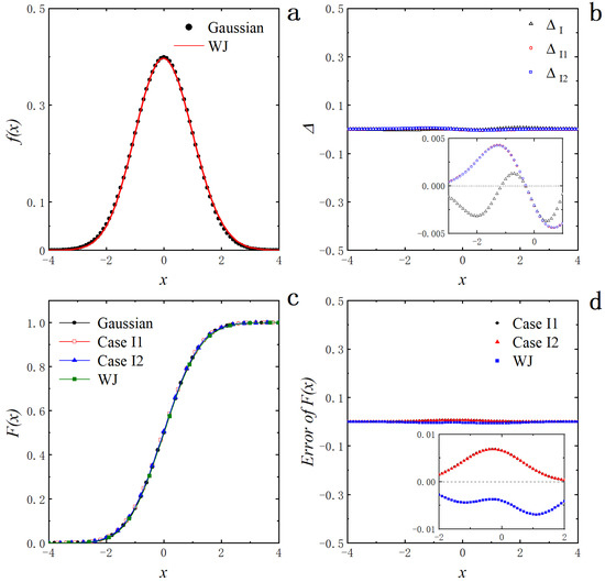
Figure 2. Analyses of expanding the WJ distribution based on Method I. (a) Scatter points of the standard normal distribution function (1b) at the intervals of 0.1 and fitting curve by the WJ function (2); (b) Symbols of${\mathsf{\Delta }}_{\mathsf{{\rm I}}}$,${\mathsf{\Delta }}_{\mathsf{{\rm I}}1}$ and ${\mathsf{\Delta }}_{\mathsf{{\rm I}}2}$ for the residuals of the WJ function,$\mathrm{N}\left({\widehat{\mu }}_{\mathsf{{\rm I}}},{\widehat{\sigma }}_{\mathsf{{\rm I}}1}\right)$ and $\mathrm{N}\left({\widehat{\mu }}_{\mathsf{{\rm I}}},{\widehat{\sigma }}_{\mathsf{{\rm I}}2}\right)$ relative to $\mathrm{N}\left(0, 1\right)$, respectively; (c) Signs of Gaussian, CaseI1, CaseI2 and WJ for the cumulative probability distribution functions of $\mathrm{N}\left(0, 1\right)$, $\mathrm{N}\left({\widehat{\mu }}_{\mathsf{{\rm I}}},{\widehat{\sigma }}_{\mathsf{{\rm I}}1}\right)$, $\mathrm{N}\left({\widehat{\mu }}_{\mathsf{{\rm I}}},{\widehat{\sigma }}_{\mathsf{{\rm I}}2}\right)$ and the WJ function, correspondingly; (d) Labels of CaseI1, CaseI2 and WJ for the residuals of the cumulative probability distribution functions of $\mathrm{N}\left({\widehat{\mu }}_{\mathsf{{\rm I}}},{\widehat{\sigma }}_{\mathsf{{\rm I}}1}\right)$,$\mathrm{N}\left({\widehat{\mu }}_{\mathsf{{\rm I}}},{\widehat{\sigma }}_{\mathsf{{\rm I}}2}\right)$ and the WJ function in comparison to $\mathrm{N}\left(0, 1\right)$, respectively.

The validity of Method I may be further verified by appraising the related cumulative probability distribution function $F\left(x\right)$. Since we consider in this work the cases such as the standard normal distribution with the meaningful values around the origin exclusively, it stays justified to take the lower limit to be a finite number, say −4, to replace −∞ in the integral $F\left(x\right)={\displaystyle {{\displaystyle \int }}_{-\infty }^x}f\left(x\right)\mathrm{d}x$ to compute the numerical solution of the cumulative probability distribution function. Figure 2c shows the cumulative probability distribution functions of $\mathrm{N}\left(0, 1\right)$, $\mathrm{N}\left({\widehat{\mu }}_{\mathsf{{\rm I}}},{\widehat{\sigma }}_{\mathsf{{\rm I}}1}\right)$, $\mathrm{N}\left({\widehat{\mu }}_{\mathsf{{\rm I}}},{\widehat{\sigma }}_{\mathsf{{\rm I}}2}\right)$ and the WJ function, denoted by the symbols of Gaussian, CaseI1, CaseI2, and WJ, respectively. It is obvious that the curves of the integrals nearly overlay one another. A more detailed manifestation is to weigh the residuals of $\mathrm{N}\left({\widehat{\mu }}_{\mathsf{{\rm I}}},{\widehat{\sigma }}_{\mathsf{{\rm I}}1}\right)$, $\mathrm{N}\left({\widehat{\mu }}_{\mathsf{{\rm I}}},{\widehat{\sigma }}_{\mathsf{{\rm I}}2}\right)$ and the WJ function relative to $\mathrm{N}\left(0, 1\right),$ and the results are summed up in Figure 2d with errors smaller than 0.01, consolidating the previous analysis.

3.1.3. Parameter Scaling Relations: Generalization

This subsection discourses a route to express the general Gaussian function by the WJ distribution. According to the analysis in the precedent section, it is straightforward that the WJ function is capable of representing the standard normal distribution function with the parameter set of ${\alpha }_0=12.52$, ${\beta }_0=0.07915$ and ${\nu }_0=63.96$. Since the general Gaussian distribution (1a), as previously noted, can be transformed to the standard normal distribution (1b) by the equation $x=\left(y-{\mu }_{GS}\right)/\sigma$, it is likely to formulate the general Gaussian function with arbitrary parameters by a set of specific parameters $\alpha$, $\beta$ and $\nu$ of the WJ function. In fact, we can transform Equations (2) to (12) below by taking advantage of rescaling [41,42]

$$f\left(x,{\alpha }^{*},{\beta }^{*},{\nu }^{*}\right)=\frac{{\beta }^{*}}{\Gamma \left({\alpha }^{*}/{\beta }^{*}\right)}{e}^{-{\alpha }^{*}\left(x-{\nu }^{*}\right)-e^{-{\beta }^{*}\left(x-{\nu }^{*}\right)}}$$

(12)

where ${\alpha }^{*}=\alpha /\sigma$, ${\beta }^{*}=\beta /\sigma$ and ${\nu }^{*}={\mu }_{GS}+\nu \sigma$ (In this paper, we assume the parameters $\alpha$, $\beta$ and $\nu$ obtained by fitting the WJ distribution to the standard normal function as the reference, that is, ${\alpha }^{*}={\alpha }_0/\sigma$, ${\beta }^{*}={\beta }_0/\sigma$ and ${\nu }^{*}={\mu }_{GS}+\sigma {\nu }_0$) to accomplish the procedure of fitting the general Gaussian distribution $y~\mathrm{N}\left(\mu ,\sigma \right)$ by the WJ distribution. The forms of Equations (2) and (12) are essentially the same, but the distinction lies in the scale change of the variables and the interpretation of the parameters. The derivation of Equation (12) has been based on the substitution of $y=x\sigma +{\mu }_{GS}$ into Equation (1b), resulting in the formulation of

$$f\left(y,\alpha ,\beta ,\nu \right)=\frac{\beta /\sigma }{\Gamma \left(\alpha /\beta \right)}{e}^{-\frac{\alpha }{\sigma }\left(y-{\mu }_{GS}-\nu \sigma \right)-e^{-\frac{\beta }{\sigma }\left(y-{\mu }_{GS}-\nu \sigma \right)}}$$

Several other useful relations involved include

$${\mu }_{WJ}{}^{*}+\frac{1}{{\beta }^{*}}\Psi \left(\frac{{\alpha }^{*}}{{\beta }^{*}}\right)={\mu }_{GS}+\sigma {\mu }_{WJ}+\frac{\sigma }{\beta }\Psi \left(\frac{\alpha }{\beta }\right),$$

$$\Gamma \left(\frac{{\alpha }^{*}}{{\beta }^{*}}\right)=\Gamma \left(\frac{\alpha }{\beta }\right),$$

$$\Psi \left(\frac{{\alpha }^{*}}{{\beta }^{*}}\right)=\Psi \left(\frac{\alpha }{\beta }\right),$$

and ${\mu }_{WJ}{}^{*}={\mu }_{GS}+\sigma {\mu }_{WJ}$.

In a subsequent section, we shall present explicit examples to illustrate the obtained expressions of the general Gaussian function by the WJ distribution.

3.1.4. Investigation of Parameter Solution Spaces of the WJ Distribution

It is known that the standard deviation $\sigma$ of a Gaussian function determines the shape of its curve, while the shape of the WJ distribution is jointly controlled by both parameters $\alpha$ and $\beta$. Thus, it is significant to study the interrelation between the estimate $\sigma$ with respect to the solution space of $\alpha$ and $\beta$. Inspecting Equations (7) and (8), we find that the estimate $\sigma$ is related to $\nu$ in addition to the parameters $\alpha$ and $\beta$. Thus, we need to initially derive the expression of $\nu$ in relation to $\alpha$ and $\beta$ in terms of the maximal value of the distribution function as the starting point of calculation. When the WJ distribution can well represent the Gaussian function, actually, the corresponding curve reflects a certain degree of axial symmetry, indicating that the extreme point should approach $x={\mu }_{GS}$. Since the mode of the WJ distribution is located at the point

$$x=\nu -\frac{1}{\beta }\mathit{ln}\frac{\alpha }{\beta },$$

it leads to

$$\nu ={\mu }_{GS}+\frac{1}{\beta }\mathit{ln}(\frac{\alpha }{\beta }).$$

(13)

Substituting Equation (13) into Equations (7) and (8), we deduce the following expressions for ${\widehat{\sigma }}_{\mathsf{{\rm I}}1}$ and ${\widehat{\sigma }}_{\mathsf{{\rm I}}2}$ (noted as $D_{\mathsf{{\rm I}}1}$ and $D_{\mathsf{{\rm I}}2}$ for the specific selection of $\nu$), respectively,

$$D_{\mathsf{{\rm I}}1}=\sqrt{\frac{1}{\alpha \beta e^{\beta {\mu }_{GS}}}}$$

(14)

and

$$D_{\mathsf{{\rm I}}2}=\frac{\Gamma \left(\alpha /\beta \right)}{\sqrt{2\pi }\beta e^{\frac{\alpha }{\beta }\left[\frac{1-e^{2\beta {\mu }_{GS}}}{2e^{\beta {\mu }_{GS}}}+ln\left(\frac{\alpha }{\beta }\right)-1\right]+\alpha {\mu }_{GS}}}$$

(15)

The parameter ${\mu }_{GS}$ is identified provided that the Gaussian function is specified. Afterward, we can solve Equations (14) and (15) for $\alpha$ and $\beta$ of the WJ function with respect to a given value of ${\mu }_{GS}$ by setting $D_{\mathsf{{\rm I}}1}$ and $D_{\mathsf{{\rm I}}2}$ to desired quantities. Figure 3 shows the solution space in the form of $\alpha$ vs. $\beta$ with $D_{\mathsf{{\rm I}}1}$ and $D_{\mathsf{{\rm I}}2}$ set to one. In detail, Figure 3a plots the relationship curves when ${\mu }_{GS}$ is set to 0, and the values of $D_{\mathsf{{\rm I}}1}$ and $D_{\mathsf{{\rm I}}2}$ are given to one. As shown in the figure, the curves are awfully sensitive to the change of $\alpha$ when $\alpha$ is less than one, whereas they become sensitive to the change in $\beta$ when $\alpha$ is greater than four. The two curves of $D_{\mathsf{{\rm I}}1}$ and $D_{\mathsf{{\rm I}}2}$ apparently overlap when $\alpha$ is greater than two, meaning that the same set of the $\alpha$ and $\beta$ values is available to make $D_{\mathsf{{\rm I}}1}=D_{\mathsf{{\rm I}}2}$ and the WJ function is anticipated to have a better characterization of the Gaussian function. As $\alpha$ decreases, the two curves grow away from each other so that $D_{\mathsf{{\rm I}}1}$ and $D_{\mathsf{{\rm I}}2}$ do not share the same solution anymore and thus cannot take one at the same time.

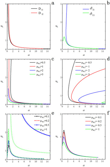
Figure 3. Effects of approximate variance $\widehat{\sigma }$ conditional upon respective mean values of ${\mu }_{GS}$ and ${\mu }_{WJ}$ on the behavior of $\alpha$ and $\beta$ in Method I. (a) Cases of $D_{\mathsf{{\rm I}}1}=1$ and $D_{\mathsf{{\rm I}}2}=1$ for ${\mu }_{GS}=0$; (b) Cases of ${\widehat{\sigma }}_{\mathsf{{\rm I}}1}=1$ and ${\widehat{\sigma }}_{\mathsf{{\rm I}}2}=1$ for ${\mu }_{WJ}=0$; (c) Sceneries of ${\widehat{\sigma }}_{\mathsf{{\rm I}}1}=1$ for positive ${\mu }_{WJ}\in \left(0.5, 1, 2, 5\right)$; (d) Sceneries of ${\widehat{\sigma }}_{\mathsf{{\rm I}}1}=1$ for negative ${\mu }_{WJ}\in \left(-5,-2,-1,-0.5\right)$; (e) Sceneries of ${\widehat{\sigma }}_{\mathsf{{\rm I}}2}=1$ for positive ${\mu }_{WJ}\in \left(0.1, 0.2, 0.5, 1\right)$; (f) Sceneries of ${\widehat{\sigma }}_{\mathsf{{\rm I}}2}=1$ for negative ${\mu }_{WJ}\in \left(-1,-0.5,-0.2,-0.1\right)$.

Instead of ${\mu }_{GS}$ by utilizing Equation (13), we can tackle the solution space of $\widehat{\sigma }$ with respect to $\alpha$ and $\beta$ by substituting

$$\nu ={\mu }_{WJ}+\frac{1}{\beta }\psi \left(\frac{\alpha }{\beta }\right)$$

into Equations (7) and (8) according to Equation (3), separately. As an adjustable parameter, ${\mu }_{WJ}$ is going to play the role of ${\mu }_{GS}$ and can be investigated with suitable values. Upon the condition of ${\widehat{\sigma }}_{\mathsf{{\rm I}}1}=1$ and ${\widehat{\sigma }}_{\mathsf{{\rm I}}2}=1$, the curves in Figure 3b depict the relationship between $\alpha$ and $\beta$ for the particular case of ${\mu }_{WJ}=0$. The trend of the curve for ${\widehat{\sigma }}_{\mathsf{{\rm I}}1}$ is analogous to that of Figure 3a, more sensitive to a change in $\alpha$. Nevertheless, ${\widehat{\sigma }}_{\mathsf{{\rm I}}2}$ appears particularly disparate: The curve first rises to the peak and then declines, displaying more sensitivity to a change in $\beta$. Figure 3c summarizes a series of curves under the conditions of ${\widehat{\sigma }}_{\mathsf{{\rm I}}1}=1$ and a set of ${\mu }_{WJ}\in \left(0.5, 1, 2, 5\right)$. When ${\mu }_{WJ}\in \left(0.5, 1\right)$, the curves have comparable trending as in Figure 3a, shifting to the left as ${\mu }_{WJ}$ increases. With ${\mu }_{WJ}$ rising from two to five, the available solution range of $\beta$ diminishes. Generally, the curves become closer for the larger $\alpha$ and the effect of ${\mu }_{WJ}$ on both $\alpha$ and $\beta$ is weakened. Figure 3d is the case of ${\widehat{\sigma }}_{\mathsf{{\rm I}}1}=1$ and ${\mu }_{WJ}\in \left(-5,-2,-1,-0.5\right)$. Of interest are the curves developing connected branches in the solution space and manifesting the shape of a boomerang [43,44]. As ${\mu }_{WJ}$ becomes smaller, the curves move to the right, and the branches become closer. In Figure 3e, branching similarly ensues in the curves of $\alpha$ vs. $\beta$ under the condition of ${\widehat{\sigma }}_{\mathsf{{\rm I}}2}=1$ and a chosen set of ${\mu }_{WJ}\in \left(0.1, 0.2, 0.5, 1\right)$, but it is a disconnected bifurcation instead. However, the scenery of branching varies significantly with smaller values of ${\mu }_{WJ}$. When ${\mu }_{WJ}\in \left(0.1, 0.2\right)$, one branch is observable in the graph, but the other branch is far away (out of the graph). As ${\mu }_{WJ}$ increases to (0.5, 1), the two separate parts of the curves gradually approach each other. The upper branch looks like the shape of an arc or a boomerang, while the lower branch is distinguishingly analogous to the case of ${\widehat{\sigma }}_{\mathsf{{\rm I}}2}=1$ and ${\mu }_{WJ}=0$ in Figure 3b, accompanied by the gradual rise of the peak value with the increase in ${\mu }_{WJ}$. In parallel, the right parts in the lower branches of the curves in the series nearly overlap, implying an insensitive contribution of ${\mu }_{WJ}$ to the change in the value of $\alpha$ and $\beta$ in the specific range. In light of Equation (8), Figure 3f exposes the solution space when ${\widehat{\sigma }}_{\mathsf{{\rm I}}2}=1$ and ${\mu }_{WJ}\in \left(-1,-0.5,-0.2,-0.1\right)$. The shapes of the curves behave like that of ${\mu }_{WJ}=0$, featuring lower peak values as ${\mu }_{WJ}$ decreases.

By the same token, we work on the behavior of the estimated mean ${\widehat{\mu }}_{\mathsf{{\rm I}}}$ as a function of $\alpha$ and $\beta$ for a reference value of ${\mu }_{WJ}$. Substituting the expression

$$\nu ={\mu }_{WJ}+\frac{1}{\beta }\Psi \left(\frac{\alpha }{\beta }\right)$$

into Equation (9) yields

$${\widehat{\mu }}_{\mathsf{{\rm I}}}=\frac{\beta e^{\beta \left[{\mu }_{WJ}+\frac{1}{\beta }\Psi \left(\frac{\alpha }{\beta }\right)\right]}-\alpha }{{\beta }^2{e}^{\beta \left[{\mu }_{WJ}+\frac{1}{\beta }\Psi \left(\frac{\alpha }{\beta }\right)\right]}}.$$

Figure 4a illustrates the 3D plot of ${\widehat{\mu }}_{\mathsf{{\rm I}}}$ as a function of $\alpha$ and $\beta$ when ${\mu }_{WJ}=0$. It is apparent that for a fixed $\beta$, ${\widehat{\mu }}_{\mathsf{{\rm I}}}$ increases with $\alpha$ and the growth gradually slows down, with the maximal value across the surface in the approach of 0. Figure 4b presents the pattern for the case of ${\mu }_{WJ}=3$, which is comparable to Figure 4a and has the maximum value near three within the displayed range of $\alpha$.

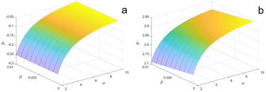
Figure 4. Three-dimensional plots of ${\widehat{\mu }}_{\mathsf{{\rm I}}}$ versus $\alpha$ and $\beta$ based on Method I. (a) Scenery of ${\mu }_{WJ}$= 0; (b) Scenery of ${\mu }_{WJ}=3$.

3.2. Method II

3.2.1. Development of the Method

This method proceeds in the way of expanding the double exponential part $e^{-\beta \left(x-\nu \right)}$ of Equation (2) around the point $x=\nu$ by the Taylor formula, i.e.,

$$e^{-\beta \left(x-\nu \right)}={\displaystyle \sum }_{n=0}^{\infty }\frac{{(-1)}^n{\beta }^n{(x-\nu )}^n}{n!},$$

converting the equation to

$$f\left(x,\alpha ,\beta ,\nu \right)=\frac{\beta }{\Gamma \left(\alpha /\beta \right)}{e}^{-\alpha \left(x-\nu \right)-{\displaystyle \sum }_{n=0}^{\infty }\frac{{(-1)}^n{\beta }^n{(x-\nu )}^n}{n!}}.$$

(16)

Provided that $\beta \left(x-\nu \right)$ is sufficiently small, the terms after ${(x-\nu )}^2$ in the sum may be cut off, and only the first three terms are retained. Thus, the Taylor series is reduced to

$${\displaystyle \sum }_{n=0}^{\infty }\frac{{(-1)}^n{\beta }^n{(x-\nu )}^n}{n!}=1-\beta \left(x-\nu \right)+\frac{{\beta }^2{(x-\nu )}^2}{2}+O[{\beta }^3{(x-\nu )}^3].$$

Subsequently, we reformulate the exponential part of Equation (16) after the truncation in a Gaussian form with a square term about $x$ and come to the deduction

$$f_{\mathsf{{\rm I}}\mathrm{I}}\left(x,\alpha ,\beta ,\nu \right)=\frac{\beta e^{\frac{{\alpha }^2-2\alpha \beta -{\beta }^2}{2{\beta }^2}}}{\Gamma \left(\alpha /\beta \right)}{e}^{-\frac{{\beta }^2{(x-\nu +\frac{\alpha }{{\beta }^2}-\frac{1}{\beta })}^2}{2}}$$

(17)

Analogous to Method I, we compare Equation (17) with the Gaussian distribution function (1a), which results in two choices of estimating the parameter $\mathsf{\sigma }$, one labeled by ${\widehat{\sigma }}_{\mathsf{{\rm I}}\mathsf{{\rm I}}1}$ from the exponential part as

$${\widehat{\sigma }}_{\mathsf{{\rm I}}\mathsf{{\rm I}}1}=\frac{1}{\beta }$$

(18)

and the other ${\widehat{\sigma }}_{\mathsf{{\rm I}}\mathsf{{\rm I}}2}$ from the pre-exponential factor as

$${\widehat{\sigma }}_{\mathsf{{\rm I}}\mathsf{{\rm I}}2}=\frac{\Gamma \left(\alpha /\beta \right)}{\sqrt{2\pi }\beta e^{\frac{{\alpha }^2-2\alpha \beta -{\beta }^2}{2{\beta }^2}}}$$

(19)

Evidently, the expression for an estimation of the mean ${\widehat{\mu }}_{\mathsf{{\rm I}}\mathsf{{\rm I}}}$ reads

$${\widehat{\mu }}_{\mathsf{{\rm I}}\mathsf{{\rm I}}}=\nu -\frac{\alpha }{{\beta }^2}+\frac{1}{\beta }$$

(20)

3.2.2. Numerical Assessment

Following the tactic employed in Method I to appraise the effectiveness of Method II, we consider the case of the standard normal distribution and replace the fitted parameter values ${\alpha }_0=12.52$, ${\beta }_0=0.07915$ and ${\nu }_0=63.96$ of the WJ distribution into Equations (18) and (19), respectively. It is immediately found that both ${\widehat{\sigma }}_{\mathsf{{\rm I}}\mathsf{{\rm I}}1}$ and ${\widehat{\sigma }}_{\mathsf{{\rm I}}\mathsf{{\rm I}}2}$ differ enormously from one, for instance, ${\widehat{\sigma }}_{\mathsf{{\rm I}}\mathsf{{\rm I}}1}$ ≈ 12.63, which is obviously much larger than one. As a consequence, the results obtained by means of the expansion in Method II may not appositely be discoursed in the same way as in Method I. In view of the discrepancy, we observe Equation (18) which shows an inverse relation between ${\widehat{\sigma }}_{\mathsf{{\rm I}}\mathsf{{\rm I}}1}$ and $\beta$. Accordingly, it exists a possibility to derive the value of $\beta$ directly from the parameter $\sigma$ of the Gaussian function and then calculate the value of α based on Equation (19). This is shown by taking the standard normal distribution as an example: Setting both ${\widehat{\sigma }}_{\mathsf{{\rm I}}\mathsf{{\rm I}}1}$ and ${\widehat{\sigma }}_{\mathsf{{\rm I}}\mathsf{{\rm I}}2}$ equal to one, it is convenient to obtain $\beta =1$ and then substitute it into Equation (19) to obtain the computed result of $\alpha \approx 1.15$. As a remark, the substitution of $\alpha$ and $\beta$ into Equation (20) results in $\nu =0.15$ under the condition of ${\widehat{\mu }}_{\mathsf{{\rm I}}\mathsf{{\rm I}}}=0$. The corresponding curve of the WJ function (2) with the calculated parameters, labeled by ${\mathrm{WJ}}_{\mathsf{{\rm I}}\mathsf{{\rm I}}}$, is shown in Figure 5a. It is transparent that the WJ function fits the Gaussian better near the peak, but the discrepancy grows bigger as $x$ moves away from the origin. The errors of the curve relative to the standard normal distribution are presented as the scatter points ${\mathsf{\Delta }}_{\mathsf{{\rm I}}\mathsf{{\rm I}}}$ in Figure 5b, plainly larger than that of Method I.

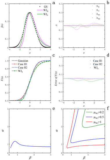
Figure 5. Analyses of expanding the WJ function by Method II around the point $x=v$. (a) ${\mathrm{WJ}}_{\mathsf{{\rm I}}\mathsf{{\rm I}}}$ based on the calculated parameters and ${\mathrm{WJ}}_0$ from fitting of the independent variable $\left(x-v\right)$; (b) ${\mathsf{\Delta }}_{\mathsf{{\rm I}}\mathsf{{\rm I}}}$, ${\mathsf{\Delta }}_0$, ${\mathsf{\Delta }}_{\mathsf{{\rm I}}\mathsf{{\rm I}}1}$ and ${\mathsf{\Delta }}_{\mathsf{{\rm I}}\mathsf{{\rm I}}2}$ for the residual scatters of the WJ function based on the calculated parameters, the WJ function fitting based on $\left(x-v\right)$, $\mathrm{N}\left({\widehat{\mu }}_{\mathsf{{\rm I}}\mathsf{{\rm I}}},{\widehat{\sigma }}_{\mathsf{{\rm I}}\mathsf{{\rm I}}1}\right)$ and $\mathrm{N}\left({\widehat{\mu }}_{\mathsf{{\rm I}}\mathsf{{\rm I}}},{\widehat{\sigma }}_{\mathsf{{\rm I}}\mathsf{{\rm I}}2}\right)$ versus $\mathrm{N}\left(0, 1\right)$, respectively; (c) Gaussian, Case$\mathsf{{\rm I}}\mathsf{{\rm I}}1$, Case$\mathsf{{\rm I}}\mathsf{{\rm I}}2$ and ${\mathrm{WJ}}_0$ for the cumulative probability distribution functions of $\mathrm{N}\left(0, 1\right)$, $\mathrm{N}\left({\widehat{\mu }}_{\mathsf{{\rm I}}\mathsf{{\rm I}}},{\widehat{\sigma }}_{\mathsf{{\rm I}}\mathsf{{\rm I}}1}\right)$, $\mathrm{N}\left({\widehat{\mu }}_{\mathsf{{\rm I}}\mathsf{{\rm I}}},{\widehat{\sigma }}_{\mathsf{{\rm I}}\mathsf{{\rm I}}2}\right)$ and the WJ function, separately; (d) Case$\mathsf{{\rm I}}\mathsf{{\rm I}}1$, Case$\mathsf{{\rm I}}\mathsf{{\rm I}}2$ and ${\mathrm{WJ}}_0$ for the residual plots of the cumulative probability distribution functions of $\mathrm{N}\left({\widehat{\mu }}_{\mathsf{{\rm I}}\mathsf{{\rm I}}},{\widehat{\sigma }}_{\mathsf{{\rm I}}\mathsf{{\rm I}}1}\right)$,$\mathrm{N}\left({\widehat{\mu }}_{\mathsf{{\rm I}}\mathsf{{\rm I}}},{\widehat{\sigma }}_{\mathsf{{\rm I}}\mathsf{{\rm I}}2}\right)$ and the WJ function obtained by fitting relative to $\mathrm{N}\left(0, 1\right)$, correspondingly; (e) Relationship between $\alpha$ and $\beta$ when ${\widehat{\sigma }}_{\mathsf{{\rm I}}\mathsf{{\rm I}}2}=1$ on the basis of Equation (19); (f) Relationship between $\alpha$ and $\beta$ assuming ${\widehat{\mu }}_{\mathsf{{\rm I}}\mathsf{{\rm I}}}=0$ with${\mu }_{WJ}\in \left(0.2, 0.5, 1\right)$ in terms of Equation (20).

Nonetheless, the value of $\sigma$ is to be determined when the Gaussian function is unknown; thus, we are not in the position to set a value to $\beta$ by applying Equation (18). We propose an alternative estimation scheme. According to Equations (16) or (17), the parameter $\nu$ appears only as$\left(x-v\right)$ in the exponential part and affects only ${\widehat{\mu }}_{\mathsf{{\rm I}}\mathsf{{\rm I}}}$. Taking the point into consideration, we could move forward by assuming ($x-v$) as the independent variable (equivalent to the case of taking $v$ = 0 which reflects the properties of some special distributions [12,13,14]). In actuality, fitting the standard normal distribution by the WJ function with ($x-v$) as the independent variable produces the parameter set of $\alpha =1.188$ and $\beta =0.9522$. The associated curve is shown by the label of ${\mathrm{WJ}}_0$ in Figure 5a and demonstrates better performance than that of ${\mathrm{WJ}}_{\mathrm{II}}$. In Figure 5b, the scatters ${\mathsf{\Delta }}_0$ chart the errors of the fitted WJ function versus the standard normal distribution. Employing Equation (20), we directly obtain ${\widehat{\mu }}_{\mathsf{{\rm I}}\mathsf{{\rm I}}}=-0.26$, which surely reveals a systematic deviation due to selecting ($x-v$) as the independent variable. We need to correct it when analyzing the truncated functions involving ${\widehat{\mu }}_{\mathsf{{\rm I}}\mathsf{{\rm I}}}$ and the magnitude of the correction is −${\widehat{\mu }}_{\mathsf{{\rm I}}\mathsf{{\rm I}}}$ or $\nu =0.26$. In Figure 5b, the symbols ${\mathsf{\Delta }}_{\mathsf{{\rm I}}\mathsf{{\rm I}}1}$ and ${\mathsf{\Delta }}_{\mathsf{{\rm I}}\mathsf{{\rm I}}2}$ represent the residual plots of $\mathrm{N}\left({\widehat{\mu }}_{\mathsf{{\rm I}}\mathsf{{\rm I}}},{\widehat{\sigma }}_{\mathsf{{\rm I}}\mathsf{{\rm I}}1}\right)$ and $\mathrm{N}\left({\widehat{\mu }}_{\mathsf{{\rm I}}\mathsf{{\rm I}}},{\widehat{\sigma }}_{\mathsf{{\rm I}}\mathsf{{\rm I}}2}\right)$ relative to $\mathrm{N}\left(0, 1\right)$ after substituting the values of $\alpha$, $\beta$ and $v$ into the equations for ${\widehat{\mu }}_{\mathsf{{\rm I}}\mathsf{{\rm I}}}$, ${\widehat{\sigma }}_{\mathsf{{\rm I}}\mathsf{{\rm I}}1}$ and ${\widehat{\sigma }}_{\mathsf{{\rm I}}\mathsf{{\rm I}}2}$. The errors are certainly larger when compared to Method I. The observation is further supported by calculating the related cumulative probability distributions, as presented in Figure 5c (where Gaussian, CaseII1, CaseII2, and ${\mathrm{WJ}}_0$ denote the cumulative probability distribution functions of$\mathrm{N}\left(0, 1\right)$, $\mathrm{N}\left({\widehat{\mu }}_{\mathsf{{\rm I}}\mathsf{{\rm I}}},{\widehat{\sigma }}_{\mathsf{{\rm I}}\mathsf{{\rm I}}1}\right)$,$\mathrm{N}\left({\widehat{\mu }}_{\mathsf{{\rm I}}\mathsf{{\rm I}}},{\widehat{\sigma }}_{\mathsf{{\rm I}}\mathsf{{\rm I}}2}\right)$ and the fitted WJ function, respectively). It is evident that the first three curves are close together as a result of the choice of the parameters, but the difference with the fitted WJ function is large. Figure 5d plots the residuals of the cumulative probability distribution functions, showing a systematic deviation of the fitted WJ distribution.

Unlike Equation (18), independent of $\alpha$ and showing a straightforward relation between ${\widehat{\sigma }}_{\mathsf{{\rm I}}\mathsf{{\rm I}}1}$ and $\beta$, Equation (19) expresses ${\widehat{\sigma }}_{\mathsf{{\rm I}}\mathsf{{\rm I}}2}$ as a complicated function of $\alpha$ and $\beta$. As before, Figure 5e plots the constraint relationship between $\alpha$ and $\beta$ for ${\widehat{\sigma }}_{\mathsf{{\rm I}}\mathsf{{\rm I}}2}=1$ with $\beta$ as the x-axis and $\alpha$ as the y-axis, portraying a feature of rapid rising to a maximum and then declining ultimately to level off. Based on Equation (20), Figure 5f exemplifies the relationship between $\alpha$ and $\beta$ with the variation of ${\mu }_{WJ}\in \left(0.2, 0.5, 1\right)$ under the condition of ${\widehat{\mu }}_{\mathsf{{\rm I}}\mathsf{{\rm I}}2}=0$. The curves are shaped like boomerangs and gradually move down to the left as ${\mu }_{WJ}$ increases.

3.2.3. An Account of the Differences between Methods I and II

We give conceivable reasoning for the different outcomes between Methods I and II. First of all, it is noticeable that the parameter $\alpha =1.188$ in Method II is much smaller than $\alpha =12.52$ in Method I, whereas the corresponding $\beta =0.9522$ is much larger than $\beta =0.07915$. In its deduction, the WJ function has assumed that a series of random variables follow exponential distributions

$$f\left(x_n\right)=\frac{\alpha +\left(n-1\right)\beta }{e}{e}^{-\left[\alpha +\left(n-1\right)\beta \right]x_n}(n=1, 2, 3, \dots ).$$

when $\beta$ is far smaller than $\alpha$, both the means and variances of the first several random variables may be considered roughly equal (and are the main contributing terms to the probability). The observation, in essence, satisfies the assumptions of the Gaussian function, and thus, the outcome of Method I discloses better characteristics in modeling the Gaussian function than that of Method II.

Referring to the computation above, either of the two expansion methods has distinct advantages itself. In Method I, the WJ distribution fits the Gaussian function much more effectively in an accurate and self-consistent manner. In Method II, the WJ distribution obtained exhibits unsatisfactory performance to fit the Gaussian function, but the expression of $\sigma$ estimation is simpler, and we may conveniently derive the parameter values of the WJ function for fitting the Gaussian distribution or as initial inputs for searching more accurate solutions.

3.3. Method III

3.3.1. Development of the Method

The WJ distribution reaches its maximum value at the point $x=x_m$ ($x_m=\nu -\ln \left(\alpha /\beta \right)/\beta$ [13]. Thus, it is a natural choice to expand the part $e^{-\beta \left(x-\nu \right)}$ in Equation (2) around $x=x_m$ on the basis of the Taylor formula, overtly,

$$e^{-\beta \left(x-\nu \right)}={\displaystyle \sum }_{n=0}^{\infty }\frac{{\left(-1\right)}^n\alpha {\beta }^{n-1}{\left(x-x_m\right)}^n}{n!},$$

resulting in the following expression for the WJ distribution

$$f\left(x,\alpha ,\beta ,\nu \right)=\frac{\beta }{\Gamma \left(\alpha /\beta \right)}{e}^{-\alpha \left(x-\nu \right)-{\displaystyle \sum }_{n=0}^{\infty }\frac{{\left(-1\right)}^n\alpha {\beta }^{n-1}{\left(x-x_m\right)}^n}{n!}}$$

(21)

Supposed that the truncation of the terms after $x^2$ is reasonable when the value of $\beta \left(x-x_m\right)$ is sufficiently small, we retain the first three terms in the way of

$$\begin{gathered} {\displaystyle {{\displaystyle \sum }}_{n=0}^{\infty }}\frac{{\left(-1\right)}^n\alpha {\beta }^{n-1}{\left(x-x_m\right)}^n}{n!}=\frac{\alpha }{\beta }-\alpha (x-x_m)+\frac{\alpha \beta {\left(x-x_m\right)}^2}{2} \\ + \mathrm{O} \left({\left(x-x_m\right)}^3\right) \end{gathered}$$

and attain the approximate expression for the WJ function

$$f_{\mathsf{{\rm I}}\mathsf{{\rm I}}\mathsf{{\rm I}}}\left(x,\alpha ,\beta ,\nu \right)=\frac{\beta }{\Gamma \left(\alpha /\beta \right)}{e}^{-\frac{\alpha \beta {(x-x_m)}^2}{2}-\frac{\alpha }{\beta }+\frac{\alpha }{\beta }\ln \frac{\alpha }{\beta }}.$$

(22)

Equation (22) is readily rearranged to the form of a Gaussian function as

$$f_{\mathsf{{\rm I}}\mathsf{{\rm I}}\mathsf{{\rm I}}}\left(x,\alpha ,\beta ,\nu \right)=\frac{\beta e^{\frac{\alpha }{\beta }\ln \frac{\alpha }{\beta }-\frac{\alpha }{\beta }}}{\Gamma \left(\alpha /\beta \right)}{e}^{-\frac{\alpha \beta {(x-x_m)}^2}{2}}$$

(23)

Associating the equation with the formulation of the Gaussian distribution function in Equation (1a), we have two possibilities for assessing the variance $\sigma$: argument of the exponential-based and pre-exponential factor-based, viz.,

$${\widehat{\sigma }}_{\mathsf{{\rm I}}\mathrm{II}1}=\sqrt{\frac{1}{\alpha \beta }}$$

(24)

and

$${\widehat{\sigma }}_{\mathsf{{\rm I}}\mathrm{II}2}=\frac{\Gamma \left(\alpha /\beta \right)}{\sqrt{2\pi }\beta e^{\frac{\alpha }{\beta }\ln \frac{\alpha }{\beta }-\frac{\alpha }{\beta }}}$$

(25)

Concerning the expectation ${\mu }_{GS}$, we acquire its estimation of ${\widehat{\mu }}_{\mathsf{{\rm I}}\mathrm{II}}$,

$${\widehat{\mu }}_{\mathsf{{\rm I}}\mathrm{II}}=x_m$$

(26)

or given in the full formula

$${\widehat{\mu }}_{\mathsf{{\rm I}}\mathrm{II}}={\mu }_{WJ}+\frac{1}{\beta }\Psi \left(\frac{\alpha }{\beta }\right)-\frac{1}{\beta }\ln \frac{\alpha }{\beta }$$

(27)

In analog to Method I, two normal distributions $\mathrm{N}\left({\widehat{\mu }}_{\mathsf{{\rm I}}\mathsf{{\rm I}}\mathsf{{\rm I}}},{\widehat{\sigma }}_{\mathsf{{\rm I}}\mathsf{{\rm I}}\mathsf{{\rm I}}1}\right)$ and $\mathrm{N}\left({\widehat{\mu }}_{\mathsf{{\rm I}}\mathsf{{\rm I}}\mathsf{{\rm I}}},{\widehat{\sigma }}_{\mathsf{{\rm I}}\mathsf{{\rm I}}\mathsf{{\rm I}}2}\right)$ are ready to formulate the WJ distribution in the form of Gaussian functions (labeled individually as CaseIII1 and CaseIII2), as explicitly described by the expressions of

$$f_{\mathsf{{\rm I}}\mathsf{{\rm I}}\mathsf{{\rm I}}1}\left(x,\alpha ,\beta ,\nu \right)=\sqrt{\frac{\alpha \beta }{2\pi }}{e}^{-\frac{\alpha \beta {(x-x_m)}^2}{2}}$$

(28)

for $\mathrm{N}\left({\widehat{\mu }}_{\mathsf{{\rm I}}\mathsf{{\rm I}}\mathsf{{\rm I}}},{\widehat{\sigma }}_{\mathsf{{\rm I}}\mathsf{{\rm I}}\mathsf{{\rm I}}1}\right)$ and

$$f_{\mathsf{{\rm I}}\mathsf{{\rm I}}\mathsf{{\rm I}}2}\left(x,\alpha ,\beta ,\nu \right)=\frac{\beta e^{\frac{\alpha }{\beta }\ln \frac{\alpha }{\beta }-\frac{\alpha }{\beta }}}{\Gamma \left(\alpha /\beta \right)}{e}^{-\pi {(\frac{\beta e^{\frac{\alpha }{\beta }\ln \frac{\alpha }{\beta }-\frac{\alpha }{\beta }}}{\Gamma \left(\alpha /\beta \right)})}^2{(x-x_m)}^2}$$

(29)

for $\mathrm{N}\left({\widehat{\mu }}_{\mathsf{{\rm I}}\mathsf{{\rm I}}\mathsf{{\rm I}}},{\widehat{\sigma }}_{\mathsf{{\rm I}}\mathsf{{\rm I}}\mathsf{{\rm I}}2}\right)$.

3.3.2. Numerical Verifications: As an Accurate, Self-Consistent Approach

As in the precedent undertakings, we aim to apply the standard normal distribution and its fit parameter set by the WJ distribution function, substituting the numbers of ${\alpha }_0=12.52$, ${\beta }_0=0.07915$ and ${\nu }_0=63.96$ into the relevant equations for analysis. Figure 6a sums up the plots for the standard normal distribution, $\mathrm{N}\left({\widehat{\mu }}_{\mathsf{{\rm I}}\mathsf{{\rm I}}\mathrm{I}},{\widehat{\sigma }}_{\mathsf{{\rm I}}\mathsf{{\rm I}}\mathrm{I}1}\right)$ and $\mathrm{N}\left({\widehat{\mu }}_{\mathsf{{\rm I}}\mathrm{I}\mathsf{{\rm I}}},{\widehat{\sigma }}_{\mathsf{{\rm I}}\mathsf{{\rm I}}\mathrm{I}2}\right)$, showing their excellent superposition in the curves. The observation is further validated by their corresponding residuals ${\mathsf{\Delta }}_{\mathsf{{\rm I}}\mathsf{{\rm I}}\mathrm{I}1}$and ${\mathsf{\Delta }}_{\mathsf{{\rm I}}\mathrm{I}\mathsf{{\rm I}}2}$ in Figure 6b. Having been used in the calculations, the estimated values of ${\widehat{\sigma }}_{\mathsf{{\rm I}}\mathrm{II}1}$= 1.0046, ${\widehat{\sigma }}_{\mathsf{{\rm I}}\mathrm{II}2}$= 1.0051 and ${\widehat{\mu }}_{\mathrm{II}\mathsf{{\rm I}}}$= −0.01647 are obtainable by substituting ${\alpha }_0$, ${\beta }_0$ and ${\nu }_0$ into Equations (24)–(26). They are basically indistinguishable from the outcomes of Method I (revealing tiny improvement if not negligible in ${\widehat{\sigma }}_{\mathsf{{\rm I}}\mathrm{II}1}$ and ${\widehat{\mu }}_{\mathrm{II}\mathsf{{\rm I}}}$ over ${\widehat{\sigma }}_{\mathsf{{\rm I}}1}$ and ${\widehat{\mu }}_{\mathsf{{\rm I}}}$, respectively). Similar to the findings in Method I, both ${\widehat{\sigma }}_{\mathsf{{\rm I}}\mathrm{II}1}$ and ${\widehat{\sigma }}_{\mathsf{{\rm I}}\mathrm{II}2}$ strikingly are nearly equal and effectively one (with the mean value ${\widehat{\mu }}_{\mathrm{II}\mathsf{{\rm I}}}$ adjacent to 0), signifying the features of the standard normal distribution function ($\sigma$= 1 and ${\mu }_{GS}$= 0). Hence, we may draw the same conclusion as in Method I that the transformation of the WJ distribution to the Gaussian function by Method III is both accurate and self-consistent.

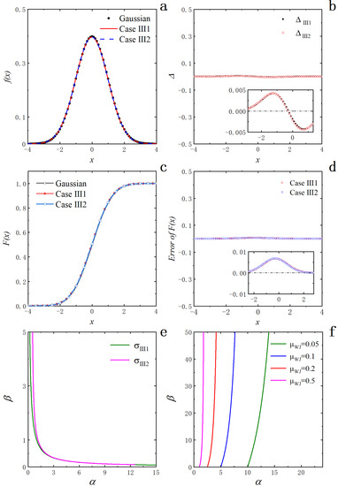
Figure 6. Analyses of expanding the WJ function by Method III performed at the mode $x=x_m$. (a) Gaussian, Case III$1$ and Case III$2$ for the standard normal distribution, $\mathrm{N}\left({\widehat{\mu }}_{\mathrm{III}},{\widehat{\sigma }}_{\mathrm{III}1}\right)$ and $\mathrm{N}\left({\widehat{\mu }}_{\mathrm{III}},{\widehat{\sigma }}_{\mathrm{III}2}\right)$, correspondingly; (b) ${\mathsf{\Delta }}_{\mathrm{III}1}$ and ${\mathsf{\Delta }}_{\mathrm{III}2}$ for the residual scatters of $\mathrm{N}\left({\widehat{\mu }}_{\mathrm{III}},{\widehat{\sigma }}_{\mathrm{III}1}\right)$ and $\mathrm{N}\left({\widehat{\mu }}_{\mathrm{III}},{\widehat{\sigma }}_{\mathrm{III}2}\right)$ versus $\mathrm{N}\left(0, 1\right)$, respectively; (c) Gaussian, Case$\mathrm{III}1$ and Case$\mathrm{III}2$ for the cumulative probability distribution functions of $\mathrm{N}\left(0, 1\right)$, $\mathrm{N}\left({\widehat{\mu }}_{\mathrm{III}},{\widehat{\sigma }}_{\mathrm{III}1}\right)$ and $\mathrm{N}\left({\widehat{\mu }}_{\mathrm{III}},{\widehat{\sigma }}_{\mathrm{III}2}\right)$, separately; (d) Case$\mathrm{III}1$ and Case$\mathrm{III}2$ for the respective residual plots of the cumulative probability distribution functions of $\mathrm{N}\left({\widehat{\mu }}_{\mathrm{III}},{\widehat{\sigma }}_{\mathrm{III}1}\right)$ and $\mathrm{N}\left({\widehat{\mu }}_{\mathrm{III}},{\widehat{\sigma }}_{\mathrm{III}2}\right)$ relative to $\mathrm{N}\left(0, 1\right)$; (e) ${\sigma }_{\mathrm{III}1}$ and ${\sigma }_{\mathrm{III}2}$ for relationship between $\alpha$ and $\beta$ when ${\widehat{\sigma }}_{\mathrm{III}1}=1$ and ${\widehat{\sigma }}_{\mathrm{III}2}=1$, respectively; (f) Relationship between $\alpha$ and $\beta$ assuming ${\widehat{\mu }}_{\mathrm{III}}=0$ with ${\mu }_{WJ}\in \left(0.05, 0.1, 0.2,0.5\right)$ according to Equation (27), individually.

Consistent with the well-defined observation above, Figure 6c evaluates the accuracy of the cumulative probability distribution functions for $\mathrm{N}\left(0, 1\right)$, $\mathrm{N}\left({\widehat{\mu }}_{\mathsf{{\rm I}}\mathrm{I}\mathsf{{\rm I}}},{\widehat{\sigma }}_{\mathsf{{\rm I}}\mathsf{{\rm I}}\mathrm{I}1}\right)$ and $\mathrm{N}\left({\widehat{\mu }}_{\mathsf{{\rm I}}\mathrm{I}\mathsf{{\rm I}}},{\widehat{\sigma }}_{\mathsf{{\rm I}}\mathsf{{\rm I}}\mathrm{I}2}\right)$, with their residuals, plotted in Figure 6d. The relationships of the parameter spaces are exemplified for ${\widehat{\sigma }}_{\mathsf{{\rm I}}\mathsf{{\rm I}}\mathrm{I}1}=1$ and ${\widehat{\sigma }}_{\mathsf{{\rm I}}\mathsf{{\rm I}}\mathrm{I}2}=1$ in Figure 6e, which are only a function of $\alpha$ and $\beta$ and show the monotonic decrease in $\beta$ with increasing $\alpha$, separately. In contrast, the estimation ${\widehat{\mu }}_{\mathsf{{\rm I}}\mathsf{{\rm I}}\mathsf{{\rm I}}}$ is a function of ${\mu }_{WJ}$ in addition to $\alpha$ and $\beta$, as delineated in Equation (27). Figure 6f is the graphs representing the relation between $\alpha$ and $\beta$ upon the selected ${\mu }_{WJ}$ for the specific case of ${\widehat{\mu }}_{\mathsf{{\rm I}}\mathsf{{\rm I}}\mathsf{{\rm I}}}=0$. Overall, the graphs display a rapid monotonic increase in $\beta$ with increasing $\alpha$. Perceptibly, the features of the parameters behave tremendously in a different way from Method I to Method III (cf. Figure 3 and Figure 6).

3.4. On the Relationship of the Three Methods

We have proposed the three methods, Methods I–III, of expanding the WJ distribution function to the Gaussian form by truncating the corresponding Taylor series. It looks stimulating to inspect their relations. Here we focus discussion on the estimation parameters of ${\widehat{\sigma }}_{\mathsf{{\rm I}}1}$ of Method I, ${\widehat{\sigma }}_{\mathsf{{\rm I}}\mathrm{I}1}$ of Method II and ${\widehat{\sigma }}_{\mathsf{{\rm I}}\mathrm{II}1}$ of Method III. In light of their expressions, ${\widehat{\sigma }}_{\mathsf{{\rm I}}\mathrm{I}1}$ is derivable from ${\widehat{\sigma }}_{\mathsf{{\rm I}}1}$ by setting $\nu$ to 0 in Equation (7) and ${\widehat{\sigma }}_{\mathsf{{\rm I}}\mathrm{II}1}$ can be obtained from ${\widehat{\sigma }}_{\mathsf{{\rm I}}1}$ by setting

$$\nu =\frac{1}{\beta }\ln \frac{\alpha }{\beta }$$

in Equation (7). Nevertheless, there is no general relation between ${\widehat{\sigma }}_{\mathsf{{\rm I}}\mathrm{I}1}$ and ${\widehat{\sigma }}_{\mathsf{{\rm I}}\mathrm{II}1}$ except for the condition of $\alpha =\beta$.

3.5. On Mutual Fitting of WJ Distributions and Arbitrary Gaussian Functions

Having performed the analysis of the relationship between the WJ distribution and the standard Gaussian function above, we now go over the capacity of the WJ distribution to fit a general Gaussian function, or vice versa, and the merits of fitting general WJ distributions by Gaussian functions. Figure 7a lists several selected examples of fitting the Gaussian function, $\mathrm{N}\left(0, 1\right)$, $\mathrm{N}\left(-1, 0.5\right)$, $\mathrm{N}\left(1, 2\right)$, and $\mathrm{N}\left(2, 5\right)$, by the WJ distribution (for convenience of later discussion, the subscripts 0, 1, 2 and 3 are assigned in order from left to right). Table 1 sums up the parameter values of the designated curves and the corresponding fitting outcomes as obtained. In the figure, each individual fitting result is in excellent agreement (Gaussian functions in solid dots and fitting WJ distributions in solid lines), as statistically reflected in their correlation coefficients of almost one (0.9997 or larger for all the examples in actual). Based on the obtained parameters in Table 1, we compute the value of ${\mu }_{WJ}$ in terms of $\nu$ and obtain ${\mu }_{WJ0}=0.0235$, ${\mu }_{WJ1}=-0.9835$, ${\mu }_{WJ2}=1.0104$ and ${\mu }_{WJ3}=2.1504$ accordingly. A more direct calculation produces the ratios of

$$\frac{{\alpha }_0}{{\alpha }_1}\approx 0.5,\frac{{\alpha }_0}{{\alpha }_2}\approx 2\mathrm{and}\frac{{\alpha }_0}{{\alpha }_3}\approx 4.96$$

as well as

$$\frac{{\beta }_0}{{\beta }_1}\approx 0.5, \frac{{\beta }_0}{{\beta }_2}\approx 1.98\mathrm{and}\frac{{\beta }_0}{{\beta }_3}\approx 4.99,$$

which are satisfactorily consistent with the previous derivations of

$${\alpha }^{*}=\frac{\alpha }{\sigma }\mathrm{and}{\beta }^{*}=\frac{\beta }{\sigma }.$$

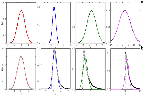
Figure 7. Mutual representation of WJ distributions and Gaussian functions (refer to Table 1 for parameter selection and fitting results). (a) Fitting of Gaussian functions (in dots) by WJ distributions (in solid line); (b) Fitting of WJ distributions (in hollow squares) by Gaussian functions (in solid line).

Table 1. Parameteric selection and fitting results for mutual fitting between Gaussian functions and WJ distributions.

	$\mathbf{\mu }$	$\mathbf{\sigma }$	$\mathbf{\alpha }$	$\mathbf{\beta }$	$\mathbf{\nu }$	${\mathit{R}}^{\mathbf{2}}$
WJ fitting GS	0	1	12.52	0.07915	63.96	0.9997
	−1	0.5	25.01	0.1575	31.17	0.9998
	1	2	6.251	0.0399	127.6	0.9998
	2	5	2.526	0.01584	322.1	0.9997
	$\mathbf{\alpha }$	$\mathbf{\beta }$	$\mathbf{\nu }$	$\mathbf{\mu }$	$\mathbf{\sigma }$	${\mathit{R}}^{\mathbf{2}}$
GS fitting WJ	12.52	0.07915	63.96	0	1	0.9997
	1	2	3	3.632	0.8439	0.9500
	2	20	5	5.305	0.3055	0.8588
	1	15	10	10.59	0.5974	0.8347

Still, setting $\delta ={\mu }_{WJ}{}^{*}-\left({\mu }_{GS}+\sigma {\mu }_{WJ}\right)$ gives the results of ${\delta }_1\approx 0.0048$, ${\delta }_2\approx -0.0366$ and ${\delta }_3=0.0329$, all of which are close to 0 as expected. Obviously, the sound fits of the Gaussian functions by the WJ distributions sanction the validity of the rescaling scheme as deduced in the section of Method I.

The scrutiny in the previous sections has attested that the WJ distribution is capable to well characterize the Gaussian function of arbitrary parameters. Next, we investigate the effect of fitting the WJ distribution by the Gaussian function. Figure 7b shows four cases of Gaussian functions fitting to WJ distributions, and Table 1 summarizes the parameters taken for the WJ distributions and the fitting results from the Gaussian functions. As indicated in the first panel of Figure 7b (WJ distribution in hollow squares and fitting Gaussian function in solid line), the fit is expectedly desired since the WJ function takes the specific set of the parameters ${\alpha }_0=12.52$, ${\beta }_0=0.07915$ and ${\nu }_0=63.96$. Combined with the preceding analysis (the WJ distribution fits almost the standard normal function), the WJ distribution and the Gaussian function can mutually represent each other with these particular parameters. This phenomenon, nonetheless, alters dependent on the set of the parameters specified when we vary the values of $\alpha$, $\beta$ and $\nu$. It is true that the second plot in Figure 7b shows a significantly unsatisfactory fit in comparison to the first, while the Gaussian functions in the third and fourth figures no longer portray properly the trends of the corresponding WJ distributions, which are enormously distinct by the difference in the peaks of the curves. Thus, it follows that Gaussian functions are not able to capture the main characteristics of the WJ function in general. Statistically, the features of the curves are overall manifested in the change in their correlation coefficients from almost one (0.9997 in actual) for the first panel declining to 0.8347 for the last panel.

The explication in the above points to the fact that if a stochastic process is describable by a Gaussian function, it can be at the same time quantified by a WJ distribution almost in the identical way; on the contrary, it may not be the case.

3.6. Analyses of Typical Cases

3.6.1. Application to Advanced Magnetism

To demonstrate the practical usefulness of the WJ distribution in preference to the Gaussian function, we first analyze a typical case in extreme events and critical phenomena as an example [45]. A set of the experimental data are extracted from the literature and fitted with the WJ distribution and the Gaussian function, respectively. The assessment is conducted by interpreting the magnetization intensity $\left(M-⟨M⟩\right)/{\sigma }_M$ as the negative variable $x$ in the WJ distribution (2) and the Gaussian function (1a) due to the positive definition of the parameters $\alpha$ and $\beta$, with the probability density scaled by the magnitude of ${\sigma }_M$. The fitting results are shown in Figure 8, yielding the fit parameters of $\alpha =1.542$, $\beta =0.7467$ and$\nu =0.5878$ ($R^2=0.9983$) for the WJ distribution and ${\mu }_{GS}=0.8879$ and $\sigma =1.28$ ($R^2=0.8091$) for the Gaussian function, separately. It is plain from the figure that the WJ function offers a well-defined matching to the experimental data with the correlation coefficient of 0.9983 (virtually one for a most optimized fit), in striking contrast to the unsatisfied performance of the Gaussian function with a rather poor correlation coefficient of 0.8091. This example strongly advocates that the WJ function has the advantage in such practical situations. In turn, we apply the WJ distribution to refit this Gaussian function of ${\mu }_{GS}=0.8879$ and $\sigma =1.28$ itself, and the outcome is given in the inset of Figure 8. As expected, both of them agree quite impressively with the parameter values of $\alpha =8.482$, $\beta =0.0764$, and$\nu =62.36$ and give a remarkable correlation coefficient of 0.9969, substantiating the proposition once more that the WJ distribution can well represent the general Gaussian function.

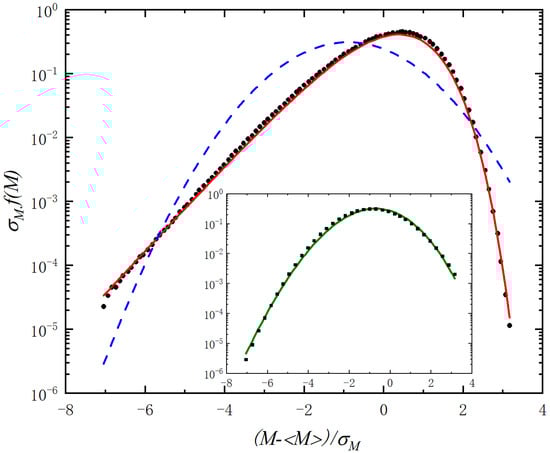
Figure 8. Comparative analysis of typical experimental data from the classical literature. Dots for experimental data, solid line for fitting of the WJ distribution and dashed line for fitting of the Gaussian function. Inset: Square solid points representing the Gaussian function obtained from the fit of the data and green solid line for the result of its refitting by the WJ distribution.

3.6.2. Application to Topical Medical Imaging Analyses

It is noteworthy that the data set considered in the above deliberation has provided an example to demonstrate the representation of the WJ distribution for the Gaussian function in addition to the pertinency to extreme events and critical phenomena. Due to its skewedness; however, a concern could arise about the legitimacy of applying the Gaussian function to it as a result of possible misinterpretation in the procedure. To resolve the issue and give more examples in practical application, we are going to present the data acquired from the same experiment [7], both with and without skewedness, to directly appraise the applicability of the WJ distribution and the Gaussian function in the following. The experiment reports a multidisciplinary fitting approach to improve the localization of parathyroid glands from their Single-Photon Emission Computed Tomography (SPECT) images using generalized Gaussian functions for quantitative assessment of preoperative parathyroid SPECT/CT (CT, Computed Tomography) scintigraphy results in a large patient cohort in combination with Particle Swarm Optimization (PSO) modeling and generates the distributions of several important parameters. Two sets of experimental data are retrieved to initiate a preliminary evaluation of the effectiveness of the Gaussian function and the WJ distribution in analyzing such cases. One is the distribution of the mean scale errors for random topology, and the other is the distribution of the mean amplitude errors for random topology. Since the data are not normalized, we need to introduce a normalization factor k ($k_{GS}$ for the Gaussian function and $k_{WJ}$ for the WJ distribution) to modify the corresponding Equations (1a) and (2) in the way of

$$f_m\left(x,{\mu }_{GS},\sigma \right)=\frac{k_{GS}}{\sqrt{2\pi }\sigma }{e}^{-\frac{{(x-{\mu }_{GS})}^2}{2{\sigma }^2}}$$

(30)

and

$$f_m\left(x,\alpha ,\beta ,\nu \right)=\frac{k_{WJ}\beta }{\Gamma \left(\alpha /\beta \right)}{e}^{-\alpha \left(x-\nu \right)-e^{-\beta \left(x-\nu \right)}}$$

(31)

Figure 9 shows the fitting results and related analyses. Figure 9a presents the outcomes on the distribution of the mean scale errors for random topology (in dots) assessed by the Gaussian function (in a continuous curve) and the WJ distribution (in dashed line) separately. It is easily recognizable that both the Gaussian function and the WJ distribution can excellently match the data points, giving virtually no discernible difference between them. The fitting parameters read $\alpha =19.06$, $\beta =0.1444$, $\nu =35.84$ and $k_{WJ}=0.1027$ ($R^2=0.9981$) for the WJ distribution and ${\mu }_{GS}=2.043$, $\sigma =0.6022$ and $k_{GS}=1026$ ($R^2=0.9980$) for the Gaussian function, correspondingly. Statistically substantiating the visual observation above, the correlation coefficients, almost one (0.9981 for the WJ distribution and 0.9980 for the Gaussian function), manifest that both of them have the same, equal goodness of fit with a slightly better performance of the WJ distribution if any. The obtained normalization factors, $k_{GS}$ and $k_{WJ}$, are essentially the same, in accord with the precise estimation of the experimental data by both the WJ distribution and the Gaussian function. As recorded in Figure 9c, the good fits are mirrored in the calculated deviations of the fittings, with no apparent preference in spreading between the WJ distribution and the Gaussian function.

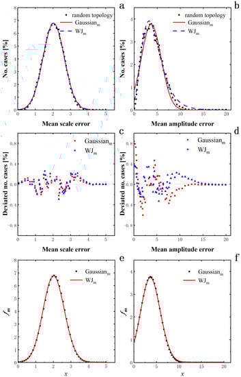
Figure 9. Comparative analyses of experimental data for different parameters obtained from the topical medical studies. (a) Distribution of mean scale errors: Experimental data (dots), Gaussian function (continuous curve) and WJ distribution (dash); (b) Distribution of mean amplitude errors: Experimental data (dots), Gaussian function (continuous curve) and WJ distribution (dash); (c) Calculated deviations of mean scale errors: Gaussian function (dots) and WJ distribution (triangles); (d) Calculated deviations of mean amplitude errors: Gaussian function (dots) and WJ distribution (triangles); (e) Fitting Gaussian function by WJ distribution for the case of mean scale errors: Gaussian function (dots) and WJ distribution (curve); (f) Fitting Gaussian function by WJ distribution for the case of mean amplitude errors: Gaussian function (dots) and WJ distribution (curve).

Figure 9b displays the fitting results on the distribution of the mean scale errors for random topology (in dots) appraised by the Gaussian function (in a continuous curve) and the WJ distribution (in dashed line) individually. In terms of the figure, both the Gaussian function and the WJ distribution can capture the major features of the data, but the performance becomes much worse for the Gaussian function than for the WJ distribution. The relevant parameters from the fittings are $\alpha =0.5157$, $\beta =0.4840$, $\nu =3.343$ and $k_{WJ}=0.2218$ ($R^2=0.9846$) for the WJ distribution and ${\mu }_{GS}=3.700$, $\sigma =2.152$ and $k_{GS}=0.2032$ ($R^2=0.9531$) for the Gaussian function, correspondingly. Examining the correlation coefficients, 0.9846 for the WJ distribution and 0.9531 for the Gaussian function, statistically reveals the degrees of deviation, which show much better performance by the WJ distribution than by the Gaussian function. Nonetheless, the acquired normalization factors, $k_{GS}$ and $k_{WJ}$, are quite different, reflecting the fact of the dissimilar estimation capabilities in gauging the experimental data between the WJ distribution and the Gaussian function. As shown in Figure 9d, such discrepancy is straightforwardly revealed in the calculated deviations of the fittings, which indicate that the maximum deviation from the Gaussian function can be twice as large as from the WJ distribution.

Subsequently, we apply the WJ distribution to refit the Gaussian function with the parameter set obtained from the fitting above. In the case of the mean scale errors, the parameter set of ${\mu }_{GS}=2.043$, $\sigma =0.6022$ and $k_{GS}=0.1026$ is used, and the fitting outcome is given in Figure 9e with the parameter values of $\alpha =20.2$, $\beta =0.1358$,$\nu =38.85$ and $k_{WJ}=0.1026$ ($R^2=0.9997$) for the fitted WJ distribution. As anticipated, the agreement between the WJ distribution and the Gaussian function is, in virtue, seamless as the correlation coefficient of 0.9997 is essentially one, confirming once more the representation of the WJ distribution for the Gaussian function. In the case of the mean amplitude errors, the parameter set is ${\mu }_{GS}=3.700$, $\sigma =2.152$ and $k_{GS}=$ 0.2032, and the fitting result is shown in Figure 9f with the parameter values of $\alpha =5.204$, $\beta =0.04077$, $\nu =122.6$ and $k_{WJ}=$ 0.2032 ($R^2=0.9997$) for the fitted WJ distribution. Analogous to the case of the mean scale errors, the superior agreement, as reflected in the outstanding correlation coefficient of 0.9997, between them proves once again the representation of the WJ distribution for the Gaussian function.

In summary, the preceding analysis shows that the WJ distribution, overall better than the Gaussian function, can give a unified approach to treating the data of the different parameters in such topical medical studies for the well-being of the patients. The unification should offer valuable insights to deepen the understanding of the experimental results and potentially facilitate the operative recovery.

4. Conclusions and Future Research

We have developed the three methods of transforming the WJ distribution to the form of the Gaussian function by means of the proper Taylor expansion, showing an accurate and self-consistent approach by expanding the double exponential part around $x=0$ (Method I) or around $x=x_m$ (Method III). The relationship between the parameters ${\mu }_{GS}$ and $\sigma$ of the Gaussian function and $\alpha$, $\beta$ and ${\mu }_{WJ}$ (or $\nu$) of the WJ distribution are systematically examined. Overall, the WJ distribution can represent the Gaussian function quite well, but the latter only fits the former satisfactorily under the condition of special sets of parameters. In addition, the parameter scaling relation of the WJ distribution to express the general Gaussian function is given. For assessing practical usefulness, we have performed the evaluation of typical cases on advanced magnetism and topical medical image processing by the WJ distribution and the Gaussian function separately. In consequence, the WJ distribution may be regarded as an extended Gaussian function, and our work initiates building up a bridge for the gap between relevant extreme value theories and Gaussian processes.

It may be appropriate to emphasize that the WJ distribution is of interest for more study owing to its suitability for circumstances subject to the Gaussian function as well as its unique potential to describe the scenery of extreme events and critical phenomena, namely, suggesting practically a unifying platform to the pertinent data processing of those quite distinct fields. In this way, future research may proceed in three aspects. (1) It is clear that Methods I and III developed in the work are accurate and self-consistent in representing the Gaussian function by the WJ distribution, but Method II shows a limited capability in doing so. As Method II has simple expressions, however, it is easy to carry out proper normalization (direct normalization) though the solution found is far from satisfactory as outlined in the section of Method II. Nevertheless, both Methods I and III possess more complicated expressions for solving and promising possibilities of direct normalization but with great challenges in finding optimized solutions if existent. Undoubtedly, it is motivating to conduct more research along the line of direct normalization in the future. (2) We have directly compared in the text the applicability of both the WJ distribution and the Gaussian function to advanced magnetism and current medical image analyses, showing a unified framework provided by the WJ distribution in preference. It is useful to broaden and deepen such initial investigations of germane experimental databases to give more insights into relevant phenomena for mechanistic understanding and advanced applications. (3) A comparison with other distributions is constructive and should put the research in a far-reaching perspective, e.g., to enrich studies in connecting pertinent extreme value theories and Gaussian processes.

References

- Krishnamoorthy, K. Handbook of Statistical Distributions with Applications; Chapman & Hall/CRC: New York, NY, USA, 2006. [Google Scholar]
- Ross, S.M. Introduction to Probability Models, 10th ed.; Elsevier: San Diego, CA, USA, 2010. [Google Scholar]
- Agresti, A.; Hitchcock, D.B. Bayesian inference for categorical data analysis. Statist. Meth. Appl. 2005, 14, 297–330. [Google Scholar] [CrossRef]
- Bryc, W. The Normal Distribution: Characterizations with Applications; Springer: New York, NY, USA, 1995. [Google Scholar]
- Deano, A.; Simm, N. Characteristic polynomials of complex random matrices and Painlev´e transcendents. Intern. Math. Res. Not. 2022, 2022, 210–264. [Google Scholar] [CrossRef]
- Gorban, A.N.; Tyukin, I.Y. Blessing of dimensionality: Mathematical foundations of the statistical physics of data. Phil. Trans. R. Soc. A 2018, 376, 20170237. [Google Scholar] [CrossRef] [PubMed]
- Listewnik, M.H.; Piwowarska-Bilska, H.; Safranow, K.; Iwanowski, J.; Laszczynska, M.; Chosia, M.; Ostrowski, M.; Birkenfeld, B.; Oszutowska-Mazurek, D.; Mazurek, P. Estimation of Parameters of Parathyroid Glands Using Particle Swarm Optimization and Multivariate Generalized Gaussian Function Mixture. Appl. Sci. 2019, 9, 4511. [Google Scholar] [CrossRef]
- Fan, S.K.S.; Lin, Y. A fast estimation method for the generalized Gaussian mixture distribution on complex images. Comput. Vis. Image Underst. 2009, 113, 839–853. [Google Scholar] [CrossRef]
- Shalliker, R.A.; Stevenson, P.G.; Shock, D.; Mnatsakanyan, M.; Dasgupta, P.K.; Guiochon, G. Application of power functions to chromatographic data for the enhancement of signal to noise ratios and separation resolution. J. Chromatogr. A 2010, 1217, 5693–5699. [Google Scholar] [CrossRef]
- Saravanan, R.; Chakraborty, A. Exact diffusion dynamics of a Gaussian distribution in one-dimensional two-state system. Chem. Phys. Lett. 2019, 731, 136567. [Google Scholar] [CrossRef]
- Souza, A.M.C.; Andrade, R.F.S.; Nobre, F.D.; Curado, E.M.F. Thermodynamic framework for compact q-Gaussian distributions. Phys. A 2018, 491, 153–166. [Google Scholar] [CrossRef]
- Stsepuro, N.; Nosov, P.; Galkin, M.; Krasin, G.; Kovalev, M.; Kudryashov, S. Generating Bessel-Gaussian Beams with Controlled Axial Intensity Distribution. Appl. Sci. 2020, 10, 7911. [Google Scholar] [CrossRef]
- Wu, J.H.; Jia, Q. A universal mechanism of extreme events and critical phenomena. Sci. Rep. 2016, 6, 21612. [Google Scholar] [CrossRef]
- Albeverio, S.; Jentsch, V.; Kantz, H. (Eds.) Extreme Events in Nature and Society; Springer: Berlin/Heidelberg, Germany, 2006. [Google Scholar]
- Fortin, J.Y.; Clusel, M. 2015 Applications of extreme value statistics in physics. J. Phys. A 2006, 48, 183001. [Google Scholar] [CrossRef]
- Bramwell, S.T. The distribution of spatially averaged critical properties. Nat. Phys. 2009, 5, 443–447. [Google Scholar] [CrossRef]
- Wu, J.H.; Jia, Q. The heterogeneous energy landscape expression of KWW relaxation. Sci. Rep. 2016, 6, 20506. [Google Scholar] [CrossRef]
- Liang, G.Y.; Xue, H.; Jia, Q.; Wu, J.H. Some Properties of the WJ Distribution and Implication in Information Theory. J. Phys. Conf. Ser. 2019, 1237, 022081. [Google Scholar] [CrossRef]
- Pisarchik, A.N.; Grubov, V.V.; Maksimenko, V.A.; Lüttjohann, A.; Frolov, N.S.; Marqués-Pascual, C.; Gonzalez-Nieto, D.; Khramova, M.V.; Hramov, A.E. Extreme events in epileptic EEG of rodents after ischemic stroke. Eur. Phys. J. 2018, 227, 921–932. [Google Scholar] [CrossRef]
- Vincze, T.; Micjan, M.; Nevrela, J.; Donoval, M.; Weis, M. Photoresponse Dimensionality of Organic Field-Effect Transistor. Materials 2021, 14, 7465. [Google Scholar] [CrossRef]
- Katsarou, A.F.; Tsamopoulos, A.J.; Tsalikis, D.G.; Mavrantzas, V.G. Dynamic Heterogeneity in Ring-Linear Polymer Blends. Polymers 2020, 12, 752. [Google Scholar] [CrossRef]
- Phillips, J.C. Stretched exponential relaxation in molecular and electronic glasses. Rep. Prog. Phys. 1996, 59, 1133–1207. [Google Scholar] [CrossRef]
- Morshedifard, A.; Masoumi, S.; Qomi, M.J.A. Nanoscale origins of creep in calcium silicate hydrates. Nat. Commun. 2018, 9, 1785. [Google Scholar] [CrossRef]
- Medina, J.S.; Arismendi-Arrieta, D.J.; Aleman, J.V.; Prosmiti, R. Developing time to frequency-domain descriptors for relaxation processes: Local trends. J. Mol. Liq. 2017, 245, 62–70. [Google Scholar] [CrossRef][Green Version]
- Qiao, J.C.; Chen, Y.X.; Pelletier, J.M.; Kato, H.; Crespo, D.; Yao, Y.; Khonik, V.A. Viscoelasticity of Cu- and La-based bulk metallic glasses: Interpretation based on the quasi-point defects theory. Mat. Sci. Eng. A-Struct. Mater. Prop. Microstruct. Proc. 2018, 719, 164–170. [Google Scholar] [CrossRef]
- Abe, H.; Yamada, T.; Shibata, K. Dynamic properties of nano-confined water in an ionic liquid. J. Mol. Liq. 2018, 264, 54–57. [Google Scholar] [CrossRef]
- Crisanto-Neto, J.C.; da Luz, M.G.E.; Raposo, E.P.; Viswanathan, G.M. An efficient series approximation for the Levy alpha-stable symmetric distribution. Phys. Lett. A 2018, 382, 2408–2413. [Google Scholar] [CrossRef]
- Aydiner, E. A Simple Model for Stretched Exponential Relaxation in Three-Level Jumping Process. Phys. Stat. Sol. B-Basic Sol. Stat. Phys. 2019, 256, 1900103. [Google Scholar] [CrossRef]
- Choi, S.; Moon, S.; Park, Y. Spectroscopic Investigation of Entropic Canopy-Canopy Interactions of Nanoparticle Organic Hybrid Materials. Langmuir 2020, 36, 9626–9633. [Google Scholar] [CrossRef]
- Aydiner, E. Memory effects and KWW relaxation of the interacting magnetic nano-particles. Phys. A 2021, 572, 125895. [Google Scholar] [CrossRef]
- Malik, A.; Kashyap, H.K. Multiple evidences of dynamic heterogeneity in hydrophobic deep eutectic solvents. J. Chem. Phys. 2021, 155, 044502. [Google Scholar] [CrossRef] [PubMed]
- Araki, T.; Gomez-Solano, J.R.; Maciolek, A. Relaxation to steady states of a binary liquid mixture around an optically heated colloid. Phys. Rev. E 2022, 105, 014123. [Google Scholar] [CrossRef]
- McKenzie, I.; Fujimoto, D.; Karner, V.L.; Li, R.H.; MacFarlane, W.A.; McFadden, R.M.L.; Morris, G.D.; Pearson, M.R.; Raegen, A.N.; Stachura, M.; et al. A beta-NMR study of the depth, temperature, and molecular-weight dependence of secondary dynamics in polystyrene: Entropy-enthalpy compensation and dynamic gradients near the free surface. J. Chem. Phys. 2022, 156, 084903. [Google Scholar] [CrossRef]
- Borelli, A.N.; Young, M.W.; Kirkpatrick, B.E.; Jaeschke, M.W.; Mellett, S.; Porter, S.; Blatchley, M.R.; Rao, V.V.; Sridhar, B.V.; Anseth, K.S. Stress Relaxation and Composition of Hydrazone-Crosslinked Hybrid Biopolymer-Synthetic Hydrogels Determine Spreading and Secretory Properties of MSCs. Adv. Healthc. Mater. 2022, 11, 2200393. [Google Scholar] [CrossRef]
- Evans, M.; Hastings, N.; Peacock, B. Statistical Distributions; John Wiley & Sons, Inc.: New York, NY, USA, 2000. [Google Scholar]
- Sabino, T.S.; Carneiro, A.M.C.; Carvalho, R.P.; Pires, F.M.A. The impact of non-Gaussian height distributions on the statistics of isotropic random rough surfaces. Trib. Inter. 2022, 173, 107578. [Google Scholar] [CrossRef]
- Azzalini, A. A class of distributions which includes the normal ones. Scand. J. Statist. 1985, 12, 171–178. [Google Scholar]
- Azzalini, A.; Capitanio, A. The Skew-Normal and Related Families; Cambridge University Press: New York, NY, USA, 2014. [Google Scholar] [CrossRef]
- Ashour, S.K.; Abdel-Hameed, M.A. Approximate skew normal distribution. J. Adv. Res. 2010, 1, 341–350. [Google Scholar] [CrossRef]
- Mudholkar, G.S.; Hutson, A.D. The epsilon–skew–normal distribution for analyzing near-normal data. J. Statist. Plan. Infer. 2000, 83, 291–309. [Google Scholar] [CrossRef]
- Kendal, W.S.; Jørgensen, B. Tweedie convergence: A mathematical basis for Taylor’s power law, 1/ f noise, and multifractality. Phys. Rev. E 2011, 84, 066120. [Google Scholar] [CrossRef] [PubMed]
- Dyre, J.C. Hidden Scale Invariance in Condensed Matter. J. Phys. Chem. B 2014, 118, 10002–10024. [Google Scholar] [CrossRef] [PubMed]
- Arnold, V.I.; Afrajmovich, V.S.; Ilyashenko, Y.S.; Shilnikov, L.P. Bifurcation Theory and Catastrophe Theory; Springer: Berlin/Heidelberg, Germany, 1994. [Google Scholar]
- Guardia, M.; Seara, T.M.; Teixeira, M.A. Generic bifurcations of low codimension of planar Filippov systems. J. Diff. Eq. 2011, 250, 1967–2023. [Google Scholar] [CrossRef]
- Bramwell, S.T.; Holdsworth, P.C.W.; Pinton, J.F. Universality of rare fluctuations in turbulence and critical phenomena. Nature 1998, 396, 552–554. [Google Scholar] [CrossRef]
Publisher’s Note: MDPI stays neutral with regard to jurisdictional claims in published maps and institutional affiliations. |
© 2022 by the authors. Licensee MDPI, Basel, Switzerland. This article is an open access article distributed under the terms and conditions of the Creative Commons Attribution (CC BY) license (https://creativecommons.org/licenses/by/4.0/).